Figures and data in Visuomotor learning from postdictive motor error

Figures
Tables
Additional files

11 figures, 1 table and 1 additional file

Figures

Figure 1

Download asset Open asset

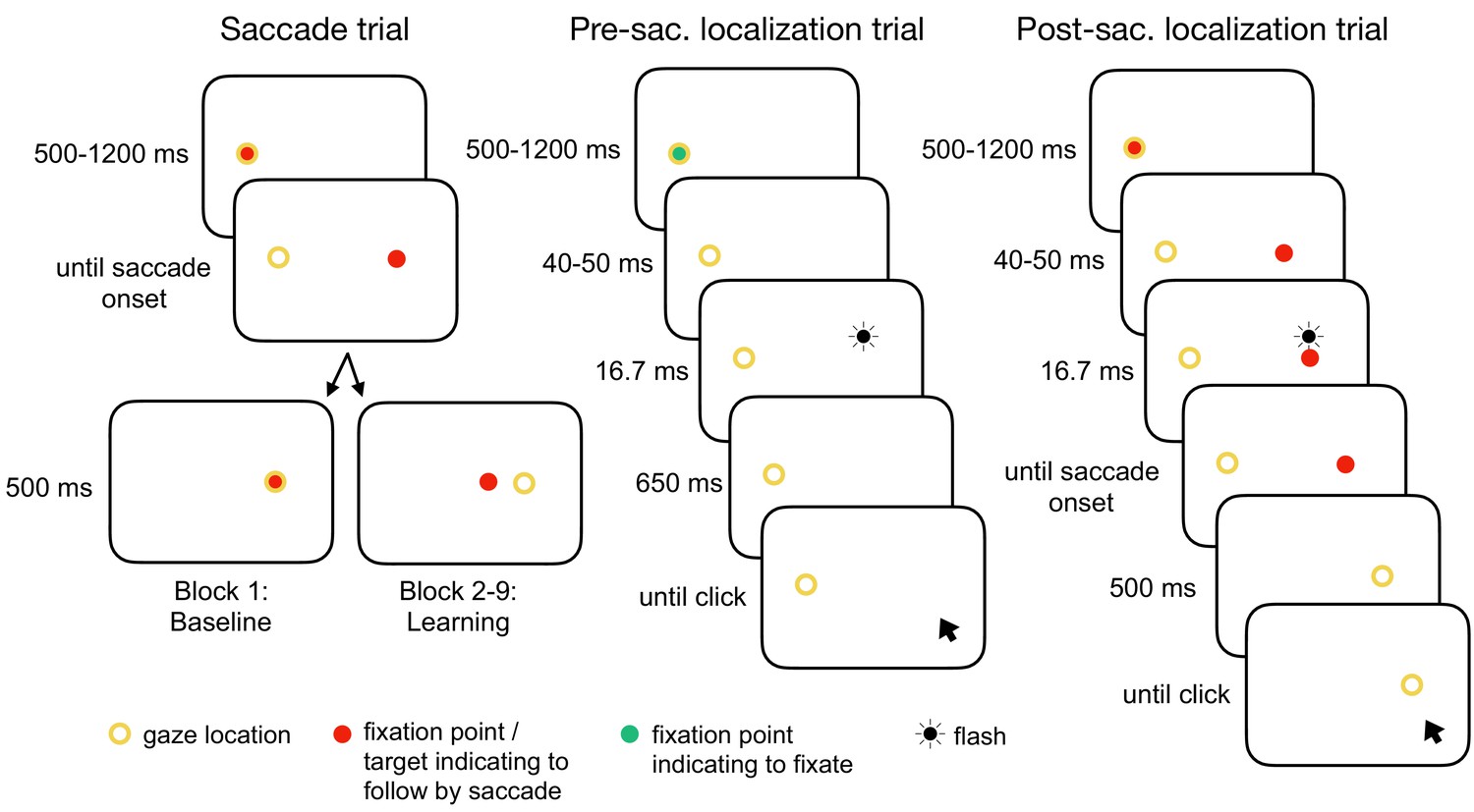
Experimental tasks.

In the saccade trials, subjects performed a reactive saccade to a 13° rightward target. During saccade execution from block 2 onwards, the target was shifted to a new location depending on the learning condition, e.g. 3° inward as shown here (CTS_in). In the pre-saccadic localization trials, subjects hold their gaze at the fixation point while localizing a white 16.7 ms flash with a gray dot cursor. In the post-saccadic localization trials, subjects performed a saccade as in the saccade trials but hold their gaze after saccade landing and report the location of the pre-saccadic flash that had appeared 40–50 ms after target onset. The yellow circle illustrates gaze location but was not present at the stimulus monitor.

Figure 2

Download asset Open asset

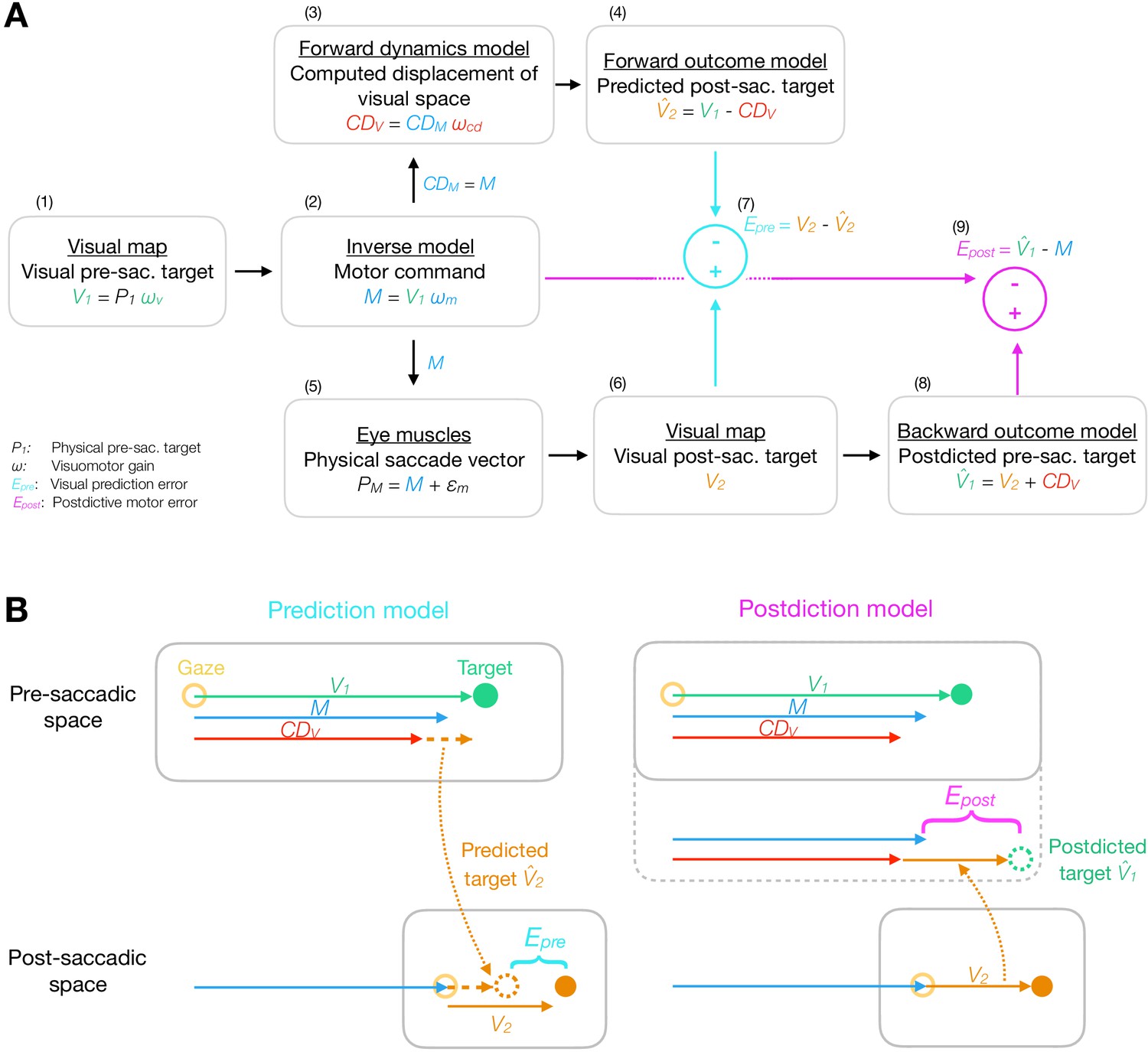
Model framework.

(A) The visual pre-saccadic target V₁ (i.e. the perceived location of a physical target P₁) is transformed into the motor command M. Before saccade execution, a forward dynamics model transforms a copy of the motor command $C D_{M}$ into a computed displacement of visual space $C D_{V}$ , a visual estimate of the saccade vector. Hence, the forward outcome model predicts the visual post-saccadic target to appear at position ${\hat{V}}_{2}$ . After saccade execution, the visual post-saccadic target appears at position V₂. According to prediction-based learning, the visuomotor system detects an error if the visual post-saccadic target deviates from its prediction ( $E_{p r e}$ ), experiencing a violation of spatial stability. According to postdiction-based learning, the visuomotor system assumes the world to remain stable during the saccade. Hence, a backward outcome model postdicts the visual post-saccadic target back to pre-saccadic space ( ${\hat{V}}_{1}$ ) in order to retroactively evaluate the motor command ( $E_{p o s t}$ ). (B) Computation of visual prediction error $E_{p r e}$ and postdictive motor error $E_{p o s t}$ . In prediction-based learning, the predicted visual error ${\hat{V}}_{2}$ is derived from the visual pre-saccadic target V₁ and the $C D_{V}$ signal in pre-saccadic space ( ${\hat{V}}_{2} = V_{1} - C D_{V}$ ) and is then compared to the actual visual error in post-saccadic space ( $E_{p r e} = V_{2} - {\hat{V}}_{2}$ ). In postdiction-based learning, the visual error V₂ is obtained in post-saccadic space and postdicted back to pre-saccadic space based on the $C D_{V}$ signal ( ${\hat{V}}_{1} = V_{2} + C D_{V}$ ). It is then compared to the original motor command to calculate postdictive motor error ( $E_{p o s t} = {\hat{V}}_{1} - M$ ).

Figure 3

Download asset Open asset

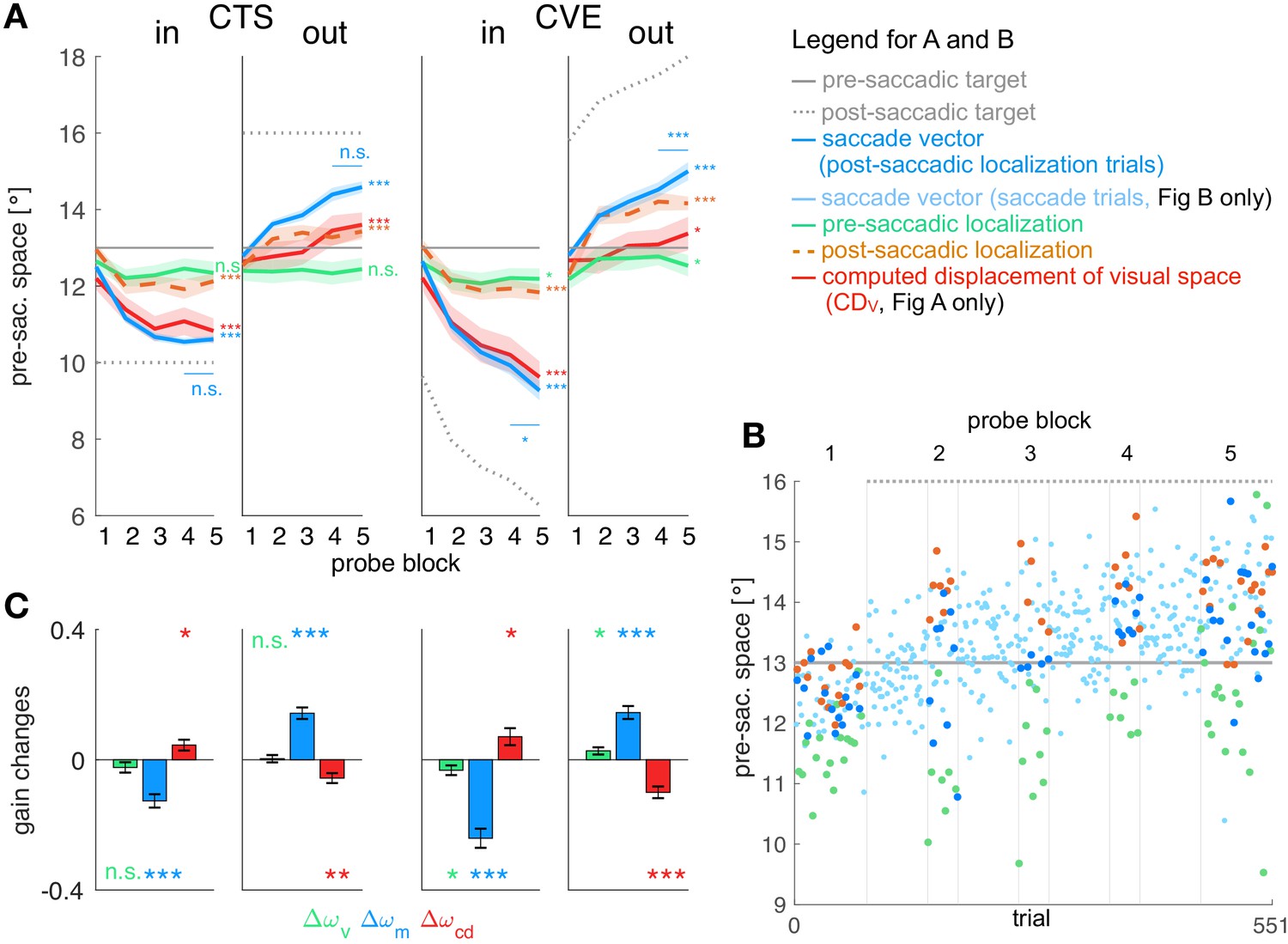
Experimental data and gain changes.

(A) Experimental data averaged across subjects. Each panel shows saccade vectors, pre- and post-saccadic localizations and $C D_{V}$ of the five probe blocks for a specific learning condition. Error bars indicate standard error of the mean. Asterisks at the right edge of each panel indicate significant change from probe block 1 to 5 with ***p<0.001, **p<0.01, *p<0.05 and n.s. p≥0.05. Blue asterisks within the panel indicate significant change from probe block 4 to 5 showing that learning was completed at the end of the CTS conditions but still in progress at the end of the CVE conditions. (B) Experimental data of an example subject for the CTS_out condition. Saccade vectors, pre- and post-saccadic localizations were measured within five probe blocks across learning. As saccade vectors needed to be related to post-saccadic localizations, only the saccade vectors of the post-saccadic localization trials (dark blue) were used for the analysis. (C) Gain changes from the first to the last trial for the four learning conditions, averaged across subjects. Asterisks indicate significant difference from zero with ***p<0.001, **p<0.01, *p<0.05 and n.s. p≥0.05.

Figure 4

Download asset Open asset

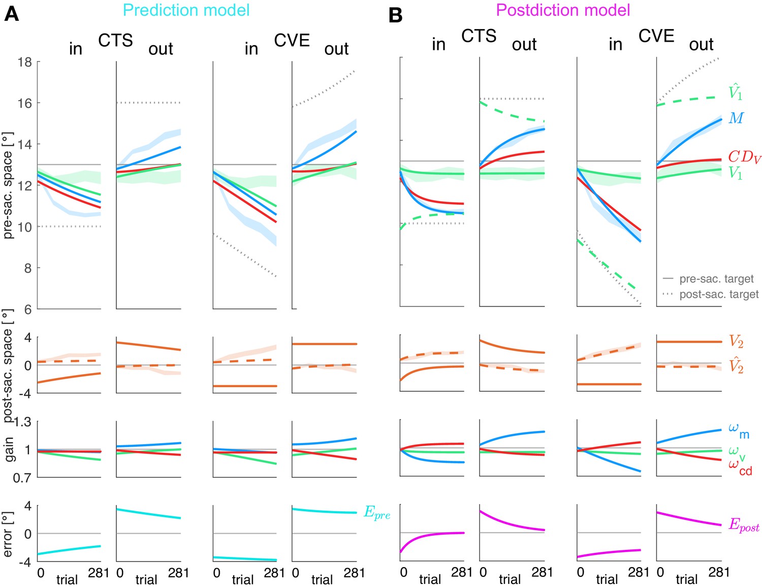
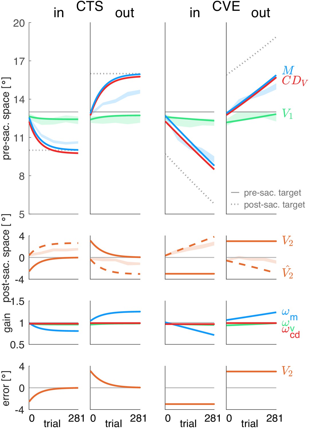
Prediction model fits and postdiction model fits to the experimental data.

Each column shows the fit for a specific learning condition. Fits are shown by lines. Data (subject means ± standard error) are shown by shaded areas. Please note that due to the model fit, the lines appear smooth compared to the mean over subjects represented by the lines in Figure 3A. First row: Visual pre-saccadic target V₁ (fitted to pre-saccadic retinal localizations, green shade), motor command M (fitted to saccade vectors, blue shade), computed displacement of visual space $C D_{V}$ , postdicted pre-saccadic target ${\hat{V}}_{1}$ in the postdiction model. Second row: Predicted post-saccadic target ${\hat{V}}_{2}$ (fitted to post-saccadic retinal localizations, orange shade), visual post-saccadic target V₂. Third row: Visual gain $ω_{v}$ , motor gain $ω_{m}$ , CD gain $ω_{c d}$ . (A) Last row: Visual prediction error $E_{p r e} = V_{2} - {\hat{V}}_{2}$ . To nullify $E_{p r e}$ , the model requires $C D_{V}$ to learn in the opposite direction of M. As this is not in line with the data, the prediction model does not adequately fit the data. Fitted learning rates are: CTS_in $α$ = (4.9*10⁻⁶; 5.0*10⁻⁵; 3.8*10⁻¹⁷), CVE_in $α$ = (4.6*10⁻⁶; 5.0*10⁻⁵; 3.4*10⁻¹⁷), CTS_out $α$ = (2.1*10⁻⁶; 5.0*10⁻⁵; 2.3*10⁻⁶), CVE_out $α$ = (2.9*10⁻⁶; 5.0*10⁻⁵; 4.0*10⁻⁶). (B) Last row: Postdictive motor error $E_{p o s t} = {\hat{V}}_{1} - M$ . At the end of the CTS conditions, $E_{p o s t} (281) \approx 0$ so that the system is appears to be converged to a steady state while at the end of the CVE conditions learning is still in progress. Fitted learning rates are: CTS_in $α$ = (5.2*10⁻⁶; 3.5*10⁻⁵; 1.8*10⁻⁵), CVE_in $α$ = (1.9*10⁻⁶; 1.3*10⁻⁵; 5.4*10⁻⁶), CTS_out $α$ = (8.4*10⁻⁸; 1.5*10⁻⁵; 6.3*10⁻⁶), CVE_out $α$ = (2.0*10⁻⁶; 9.9*10⁻⁶; 8.0*10⁻⁶).

Figure 5

Download asset Open asset

Residual standard error and visuomotor steady states.

(A) Residual standard error of the prediction and the postdiction model fit (subject means ± standard error). (B) Baseline $E_{p r e}$ and baseline $E_{p o s t}$ if no target step occurs (CTS with $P_{s}$ = 0, subject means ± standard error). The baseline error should be close to zero as the system is assumed to be in a steady state. (C) Final $E_{p r e}$ of the prediction model fit and final $E_{p o s t}$ of the postdiction model fit (subject medians with 25% and 75% quantiles). The final error should be close to zero if the system converged to a new steady state. (D) Percentage of $E_{p r e}$ decline of the prediction model fit and $E_{p o s t}$ decline of the postdiction model fit from the first trial (including target step) to the last trial (subject medians with 25% and 75% quantiles). Black asterisks indicate significant difference between prediction and postdiction model values, colored asterisks for baseline and final error indicate significant difference from zero. (E) Vector fields depict non-isolated fixed points for the baseline situation without target step and the four learning conditions (in the $ω_{m} - ω_{c d}$ plane for simplicity). Subject median $ω_{v}$ of the first trial (for baseline) and the last trial (for learning in the respective condition) and median $α$ from the respective learning conditions were chosen to draw the vector field. Subjects were at visuomotor steady state in the baseline and learned in the direction of the shifted fixed points during learning. (F) The $C D_{V}$ error determines how much visual endpoint error (visual post-saccadic target eccentricity) is left in the baseline adapted steady state of the CTS conditions (subject means ± standard error). Please note that $- (C D_{V} - M)$ , not $+ (C D_{V} - M)$ , is depicted for easier comparison to V₂. Black asterisks indicate significant difference from zero with ***p<0.001, **p<0.01, *p<0.05 and n.s. p≥0.05.

Appendix 1—figure 1

Download asset Open asset

Simulations of a model that minimizes visual error.

Each column shows the simulation for a specific learning condition. Simulations are shown by lines. Data (means ± standard error) are shown by shaded areas. First row: Visual pre-saccadic target V₁ (and pre-saccadic retinal localization data, green shade), motor command $M$ (and saccade vector data, blue shade) and computed displacement of visual space $C D_{V}$ . Second row: Predicted post-saccadic target ${\hat{V}}_{2}$ (and post-saccadic retinal localization data, orange shade), visual post-saccadic target V₂ (visual error). Third row: Visual gain $ω_{v}$ , motor gain $ω_{m}$ , CD gain $ω_{c d}$ . Last row: shows again the visual post-saccadic target V₂ (visual error) that is the error signal to be nullified. To nullify V₂, the model requires $M$ to learn until the saccade lands on the post-saccadic target. This is not in line with the data. Instead, learning converges at an earlier stage with a remaining, non-zero visual error V₂. Hence, the visual error model cannot adequately explain learning. Please note that the CD gain $ω_{c d}$ stays stable as the visual error V₂ does not depend on $C D_{V}$ such that the gradient descent procedure produces zero learning of the CD gain.

Appendix 1—figure 2

Download asset Open asset

Simulations of the postdiction model without plasticity of the CD gain ( $α_{c d}$ =0).

Each column shows the simulation for a specific learning condition. Simulations are shown by lines. Data (means ± standard error) are shown by shaded areas. First row: Visual pre-saccadic target V₁ (and pre-saccadic retinal localization data, green shade), motor command $M$ (and saccade vector data, blue shade), computed displacement of visual space $C D_{V}$ , postdicted pre-saccadic target ${\hat{V}}_{1}$ . Second row: Predicted post-saccadic target ${\hat{V}}_{2}$ (and post-saccadic retinal localization data, orange shade), visual post-saccadic target V₂. Third row: Visual gain $ω_{v}$ , motor gain $ω_{m}$ , CD gain $ω_{c d}$ . Last row: Postdictive motor error $E_{p o s t}$ . If the CD gain is not plastic and hence, stays at baseline level as shown here, $C D_{V}$ almost correctly reflects the saccade vector during learning such that the post-saccadic target localization matches the pre-saccadic target localization. This can be seen in the predicted post-saccadic target position ${\hat{V}}_{2}$ that, however, does not match the data (second row). Moreover, a non-plastic CD gain requires the saccade vector to adapt until the saccade lands on the post-saccadic target to nullify the postdictive motor error $E_{p o s t}$ . Hence, without CD plasticity the model cannot adequately explain the data.

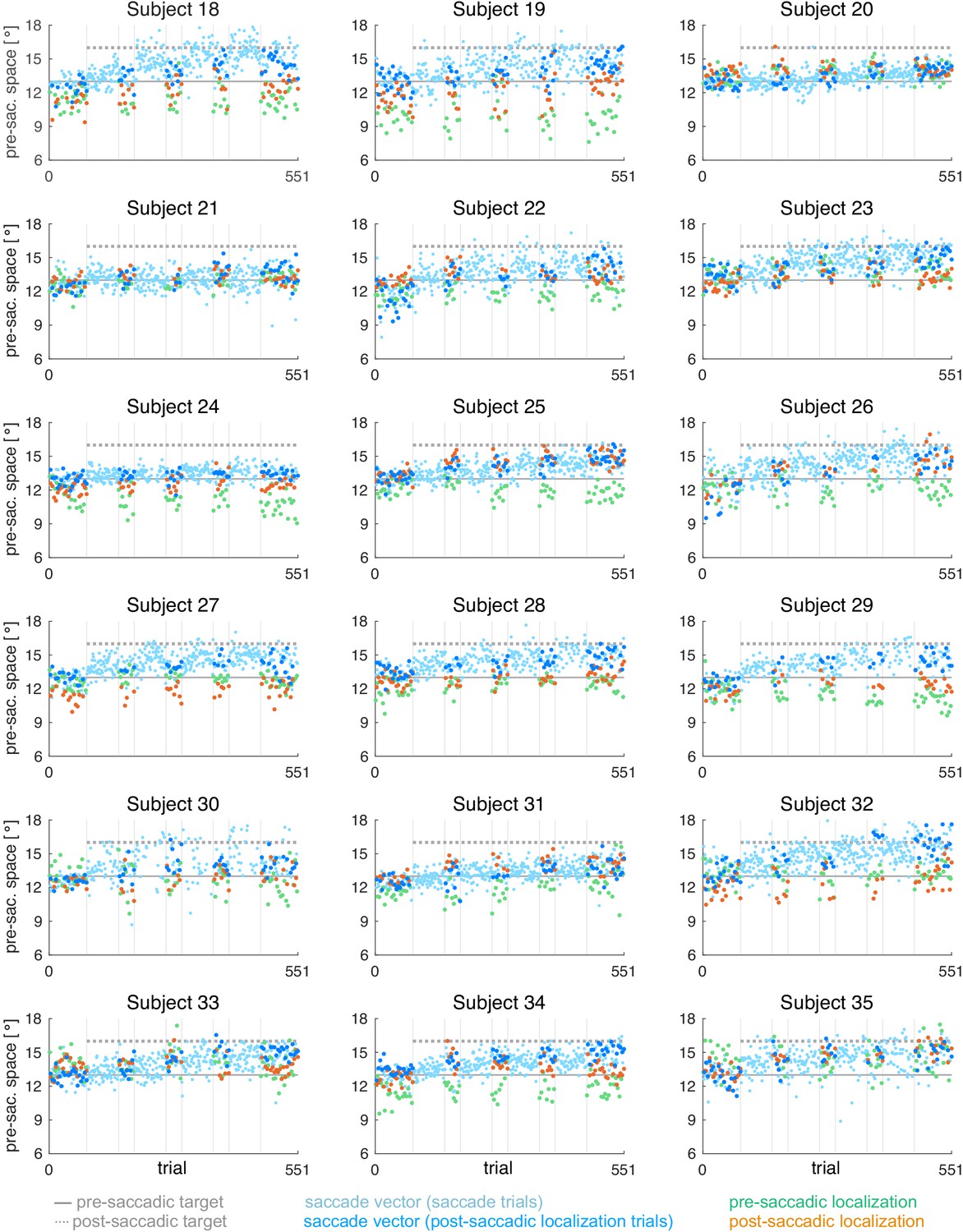
Appendix 1—figure 3

Download asset Open asset

Individual subject data for the CTS_in condition (subjects 1–17, $N$ = 17).

During the saccade, the target was shifted 3º inward (opposite to saccade direction).

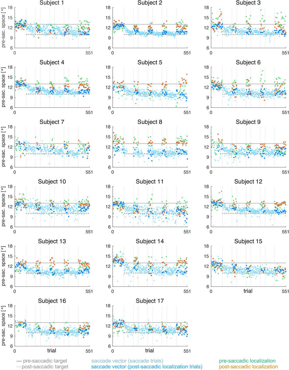
Appendix 1—figure 4

Download asset Open asset

Individual subject data for the CTS_out condition (subjects 18–35, $N$ = 18).

During the saccade, the target was shifted 3º outward (in saccade direction).

Appendix 1—figure 5

Download asset Open asset

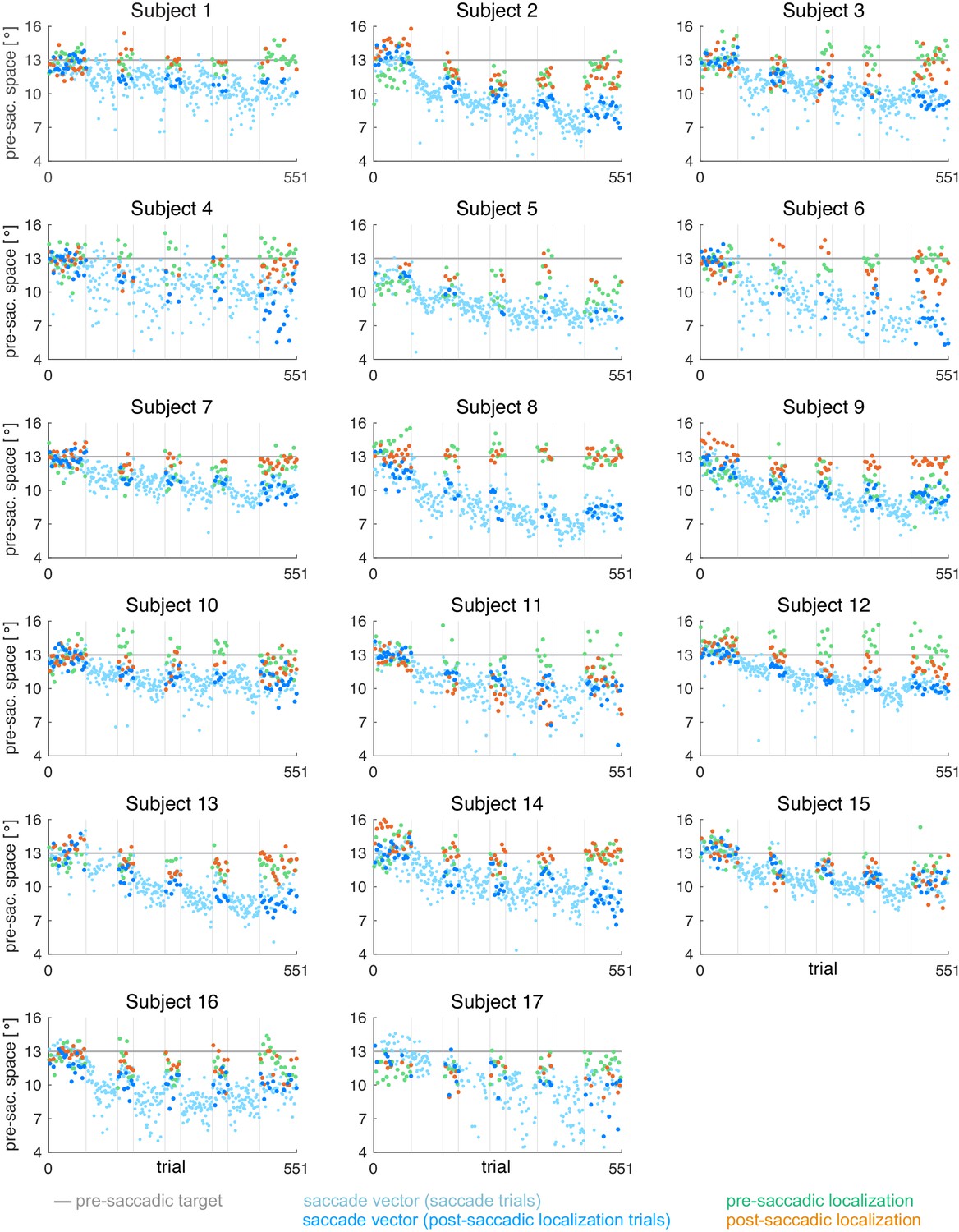
Individual subject data for the CVE_in condition (subjects 1–17, $N$ = 17).

During the saccade, the target was shifted to the position that is 3º inward (opposite to saccade direction) of the post-saccadic gaze direction.

Appendix 1—figure 6

Download asset Open asset

Individual subject data for the CVE_out condition (subjects 18–35, $N$ = 18).

During the saccade, the target was shifted to the position that is 3º outward (in saccade direction) of the post-saccadic gaze direction.

Tables

Table 1

Analysis of the experimental data.

Here, we report mean and standard deviation of changes in saccade vector, pre- and post-saccadic localization from probe block 1 to 5. T-values are derived from two-sided t-tests against zero. F-values are derived from 2 × 2 mixed ANOVAs for saccade vector, pre- and post-saccadic localization changes (corrected for direction) with paradigm (CTS/CVE) as within-subject factor and direction (in/out) als between-subject factor. Changes in saccade vector were significant in all conditions but higher for inward than outward learning (within the CVE conditions, post-hoc t-test t₃₃ = 3.68, p<0.001) and higher for CVE than CTS learning (within the inward conditions, post-hoc t-test t₃₂ = 4.94, p<0.001, CVE_in vs. CTS_out t₃₃ = −5.13, p<0.001, all other post-hoc tests p≥0.126, bonferroni-corrected significance level 0.008). Changes in post-saccadic localization were significant in all conditions but higher for CVE than CTS learning (within the outward conditions, post-hoc t-test t₃₄ = −4.23, p<0.001, CVE_out vs. CTS_in t₃₃ = −4.48, p<0.001, CVE_out vs. CVE_in t₃₃ = −2.42, p=0.021, all other post-hoc tests p≥0.163, bonferroni-corrected significance level 0.008). Changes in pre-saccadic localization were small but significant in the CVE conditions.

	Pre-saccadic localization	Saccade vector	Post-saccadic localization
CTS_in	−0.31 ± 0.85°, $t_{16}$ = −1.48, p = 0.159	−1.89 ± 0.61°, $t_{16}$ = −12.69, p < 0.001***	−0.82 ± 0.65°, $t_{16}$ = −5.24, p < 0.001***
CTS_out	+0.04 ± 0.62°, $t_{17}$ = 0.30, p = 0.766	+1.79 ± 0.71°, $t_{17}$ = 10.80, p < 0.001***	+0.88 ± 0.67°, $t_{17}$ = 5.57, p < 0.001***
CVE_in	−0.42 ± 0.80°, $t_{16}$ = −2.17, p = 0.046*	−3.37 ± 1.08°, $t_{16}$ = −12.88, p < 0.001***	−1.20 ± 0.87°, $t_{16}$ = −5.66, p < 0.001***
CVE_out	+0.35 ± 0.62°, $t_{17}$ = 2.44, p = 0.026*	+2.19 ± 0.80°, $t_{17}$ = 11.59, p < 0.001***	+1.85 ± 0.70°, $t_{17}$ = 11.17, p < 0.001***
paradigm	$F_{1, 31}$ = 3.48, p = 0.071	$F_{1, 31}$ = 31.95, p < 0.001***	$F_{1, 31}$ = 24.60, p < 0.001***
direction	$F_{1, 31}$ = 0.56, p = 0.462	$F_{1, 31}$ = 8.24, p = 0.007**	$F_{1, 31}$ = 2.94, p = 0.096
interaction	$F_{1, 31}$ = 0.76, p = 0.390	$F_{1, 31}$ = 10.75, p = 0.002**	$F_{1, 31}$ = 4.75, p = 0.036*