Topological signatures in regulatory network enable phenotypic heterogeneity in small cell lung cancer
- Centre for BioSystems Science and Engineering, Indian Institute of Science, India
- Undergraduate Programme, Indian Institute of Science, India
Figures
Figure 1
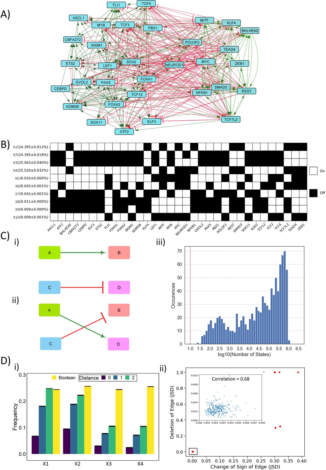
Dynamic simulations of SCLC network.
(A) SCLC regulatory network, in which green nodes denote activation and red nodes denote inhibitory interaction. (B) Steady states achieved from asynchronous Boolean update, using Ising model and 220 initial conditions (for results corresponding to 225 initial conditions, see Supplementary file 1a). Each row is a steady state, and each column is a node in the network. Dark cells represent node ‘off’ (0) and blank ones represent node ‘on’ (1). The frequency of each state is reported to the left of each row in percentage as mean ± standard deviation over three replicates. (C) (i–ii) Schematic representing edge swapping strategy for network randomization, where (ii) is a randomized network for the ‘wild-type’ (WT) network (i). (iii) Distribution of number of steady states for 1000 randomized networks corresponding to SCLC WT network. Red line shows the number of states obtained for the SCLC WT network. (D) (i) Comparison of steady-state frequencies obtained via RACIPE and Boolean. The frequency of four dominant states obtained in Boolean (X1–X4) is shown in yellow bars. The other three bars show the frequency of RACIPE states identical to corresponding Boolean states (distance = 0) and the cumulative frequency of states which are less than or equal to n nodes having different values (node value = 0 in RACIPE and 1 in Boolean or vice versa) (distance = 1, 2). Results over three replicates are reported as mean ± standard deviation (error bars). (ii) Correlation plot between Jensen–Shannon divergence (JSD) for the case of edge deletion and JSD for the case of reverting the sign of the corresponding edge. Each dot denotes an edge that has been perturbed. Inset shows zoomed-in view for the highlighted small box. The mean and standard deviation of Pearson’s coefficient correlation values for this scatter plot, over three replicates, is 0.851 ± 0.003.
Figure 2
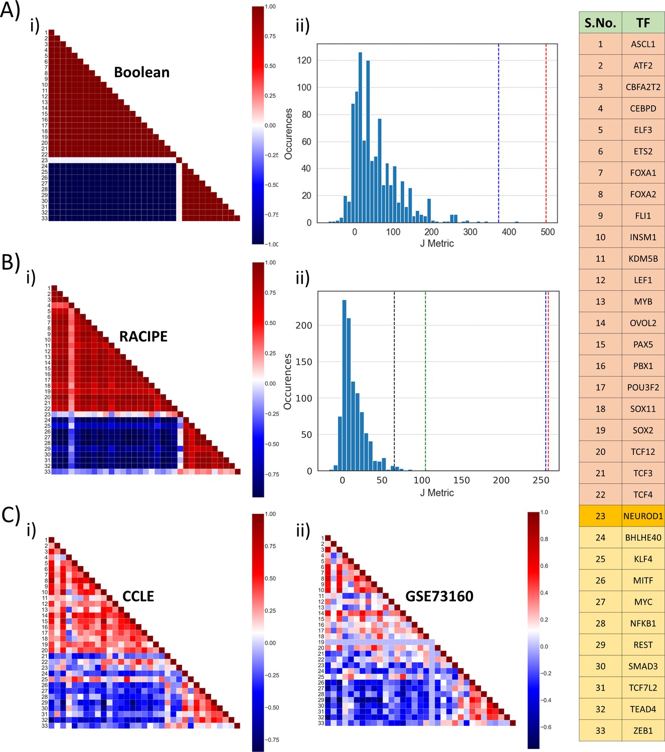
Identification of two ‘teams’.
(A) (i) Pearson’s correlation matrix for Boolean simulations of WT SCLC network. Each node represents the correlation coefficient for pairwise correlations, as shown in adjacent colormap. (ii) Distribution of the values of J metric for 1000 random networks for Boolean simulations. Red dotted line shows the value of J (=496) for Boolean simulations (A, i); blue dotted line shows the same (J = 373.05) for RACIPE simulations (B, i). (B) (i) Same as (A, i) but for RACIPE simulations. (ii) Same as (B, ii) but for cases when Pearson’s correlation coefficient values are sampled continuously from [−1,1]. Red dotted line shows the value of J for wild-type Boolean (A, i) and blue dotted line shows the value of J for Wild-type RACIPE (B, i). Black and green dotted lines show the value of J for CCLE (C, i) and GSE73160 (C, ii). (C) Same as (A, i) but for CCLE (i) and GSE73160 (ii). Details of indices 1–33 are available in the rightmost table.
Figure 3 with 2 supplements
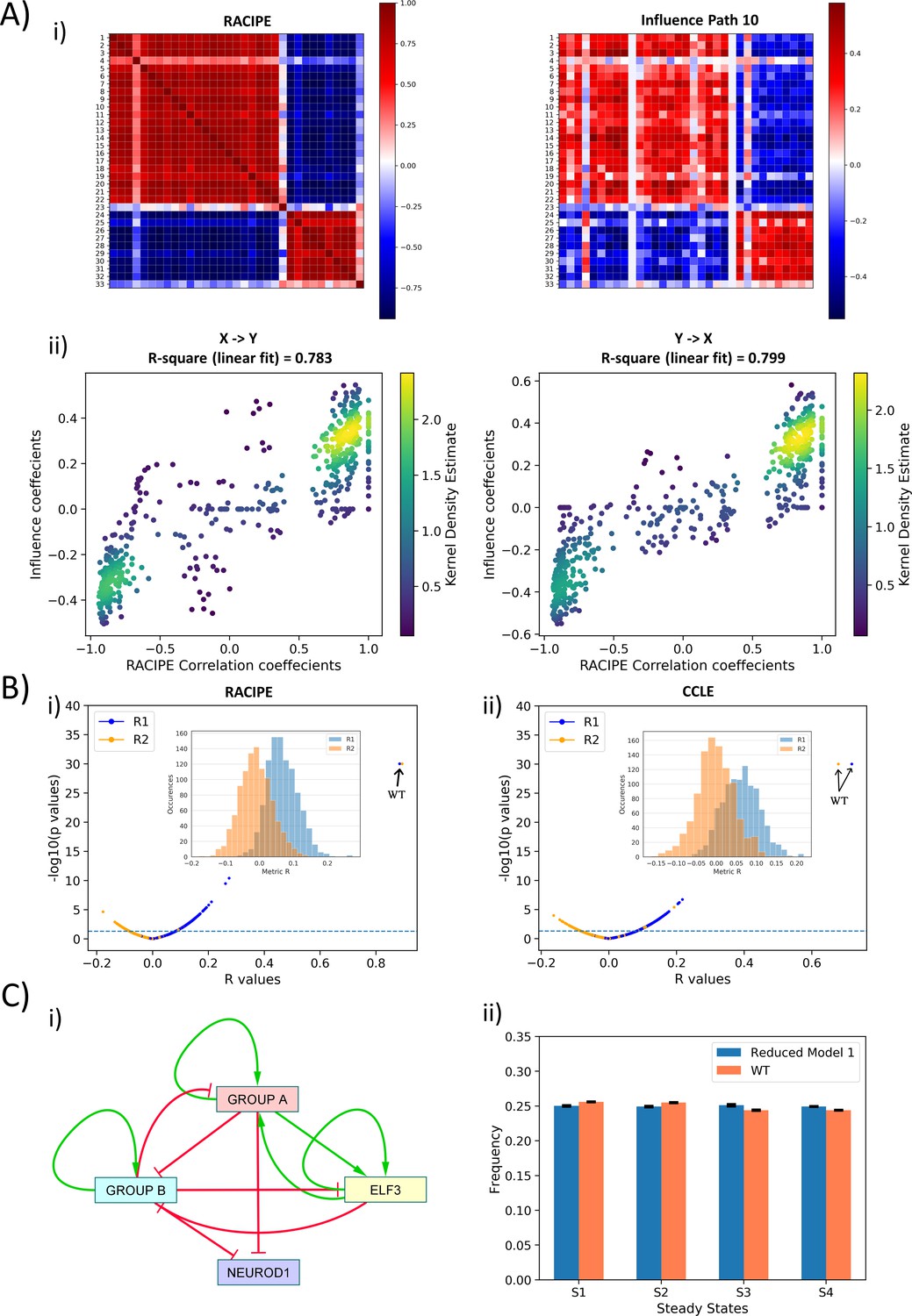
Topological features underlying the two ‘teams’ in SCLC network.
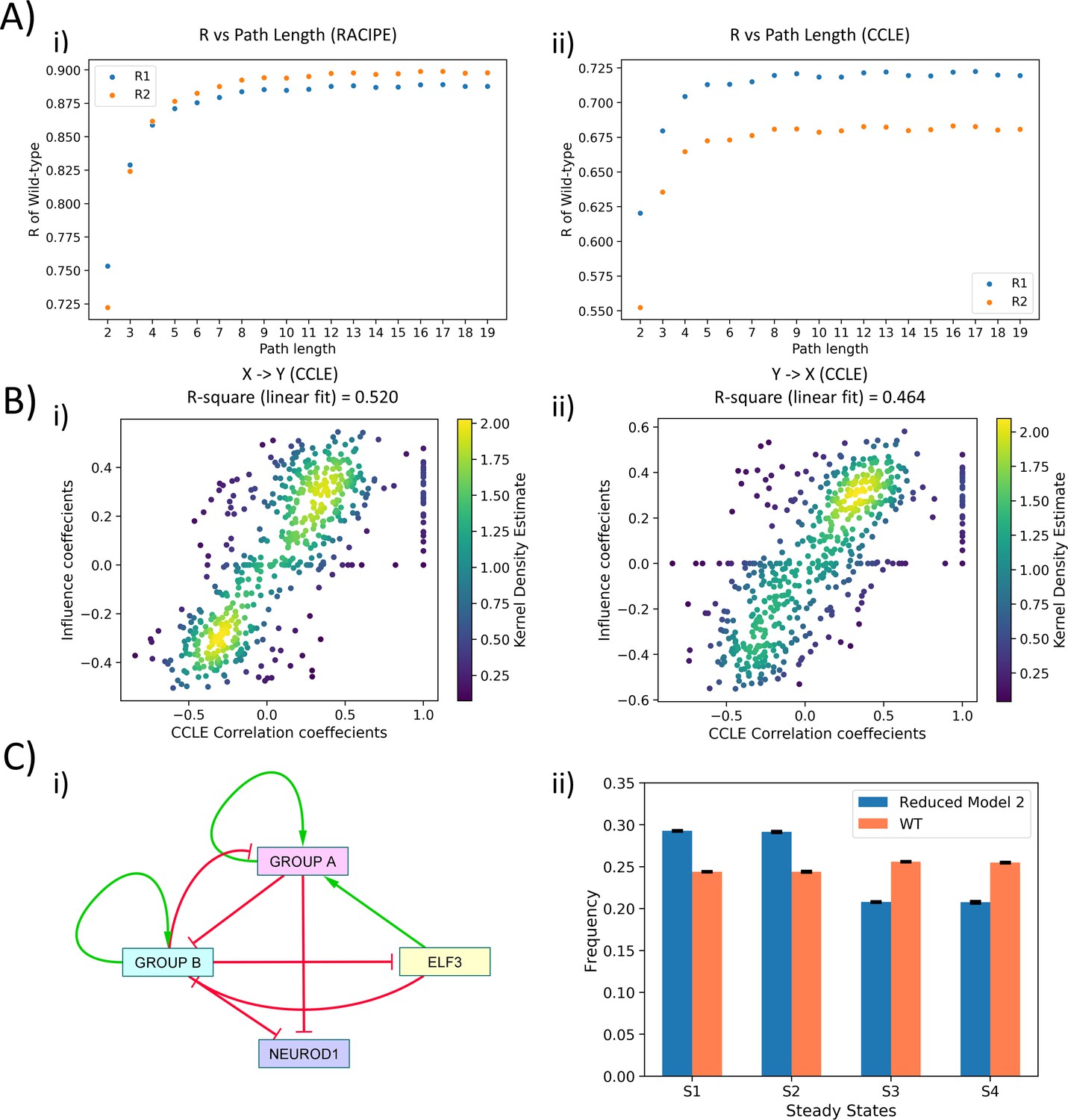
(A) (i) (Left) Pearson’s correlation matrix P for RACIPE simulations of WT SCLC network (Pij = Pji). (Right) Influence matrix Inf for WT SCLC network for path length = 10. Heatmap denotes Pij and Infij values, respectively. (ii) (left) Scatter plot for Pij and Infij values (for i < j, i.e. values in upper triangle of Inf and P matrices); (right) scatter plot for Pji and Infji values (for i > j, i.e., values in upper triangle of Inf and P matrices). R1 and R2 denote corresponding correlation coefficient values. Colorbar represents Kernel density estimate of points in the scatter plot. (B) (i) Volcano plot of all R1 and R2 metrics for RACIPE WT correlation matrix and random networks’ influence matrices. Inset shows histogram of R1 and R2 values for corresponding cases. Horizontal line for p=0.05. Arrows point to R1 and R2 values of WT SCLC network. (ii) Same as (i) but for correlation matrix from CCLE. (C) (i) Reduced model derived from influence matrix; red bars show inhibition, and green arrows show activation. (ii) Steady-state frequencies obtained from reduced model one and that of WT SCLC network (n = 3).
Figure 3—figure supplement 1
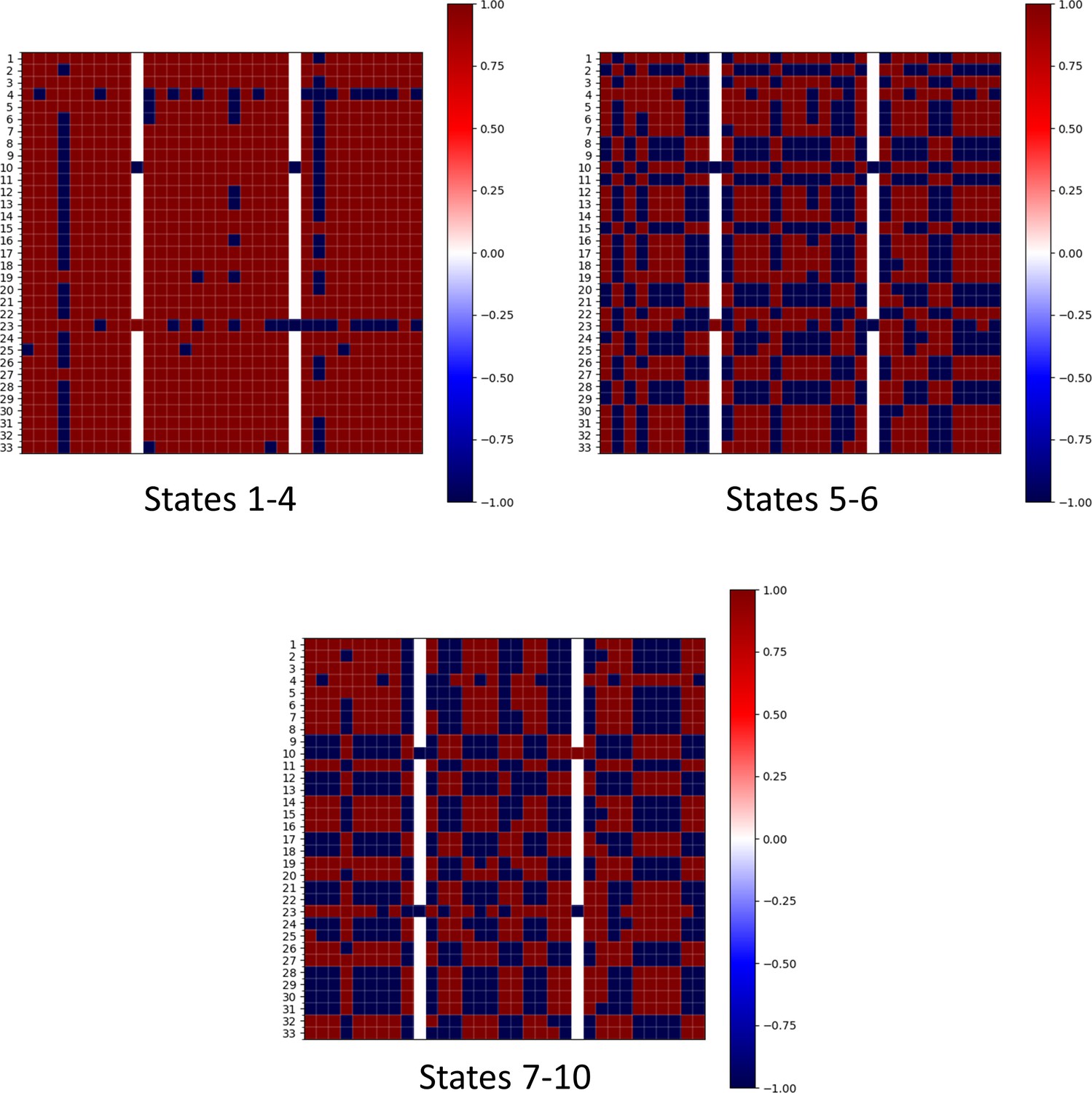
Influence matrix based on Boolean simulations for states with various frustration levels Influence matrix in Figure 3A,i is based on simulations from RACIPE.
Influence matrices based on Boolean simulation results were also derived. Instead of taking all steady-state solutions together, we classified them into three categories – states 1–4 in Supplementary file 1a (frustration value = 0.142), states 5–6 (frustration = 0.375), and states 7–10 (frustration = 0.383–0.386) – and derived corresponding influence matrices shown above. Labels 1–33 are the same as in Figure 2. The larger the frustration (or the smaller the frequency), the more the deviation of influence matrix from the correlation matrix shown in Figure 2.
Figure 3—figure supplement 2
Topological features.
(A) Scatter plot of R1 and R2 values obtained for varying path lengths, when influence matrix values/coefficients (for varying path lengths) for WT SCLC network were regressed against correlation coefficients from (i) RACIPE and (ii) CCLE. (B) (i) Scatter Plot of R1 and R2 values of influence coefficients of WT network and CCLE correlation coefficients for path length = 10. (C) (i) Reduced model derived from interaction matrix; red bars show inhibition, and green arrows show activation. (ii) Steady-state frequencies obtained from reduced model one and that of WT SCLC network (n = 3).
Figure 4 with 3 supplements
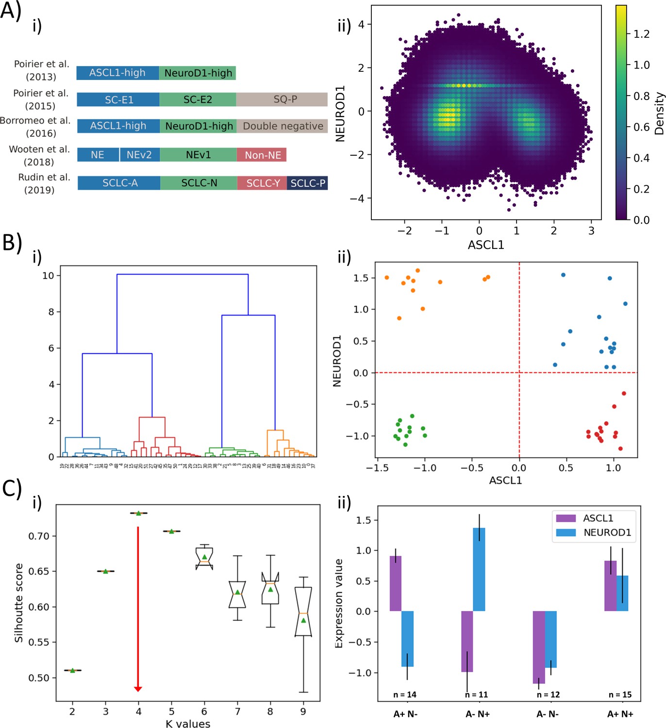
Classification of SCLC phenotypes based on ASCL1 and NEUROD1.
(A) (i) Summary of classification of SCLC subtypes in the existing literature (adapted from Rudin et al., 2019). (ii) Density-based scatter plot for ASCL1 and NEUROD1 levels, as obtained via RACIPE modeling. (B) (i) Hierarchical clustering of CCLE samples using ASCL1 and NEUROD1. (ii) Scatter plot of normalized gene expression data for CCLE samples for NEUROD1 and ASCL1. Color coding in dendrogram and scatter plot are synonymous (i.e. refer to the same cluster). (C) (i) Average Silhouette width for different values of K for K-means clustering of CCLE samples for NEUROD1 and ASCL1. Error bars denote replicates of clustering attempts. (ii) Number of samples and ASCL1 and NEUROD1 expression values as seen in four clusters of CCLE samples obtained for K = 4.
Figure 4—figure supplement 1
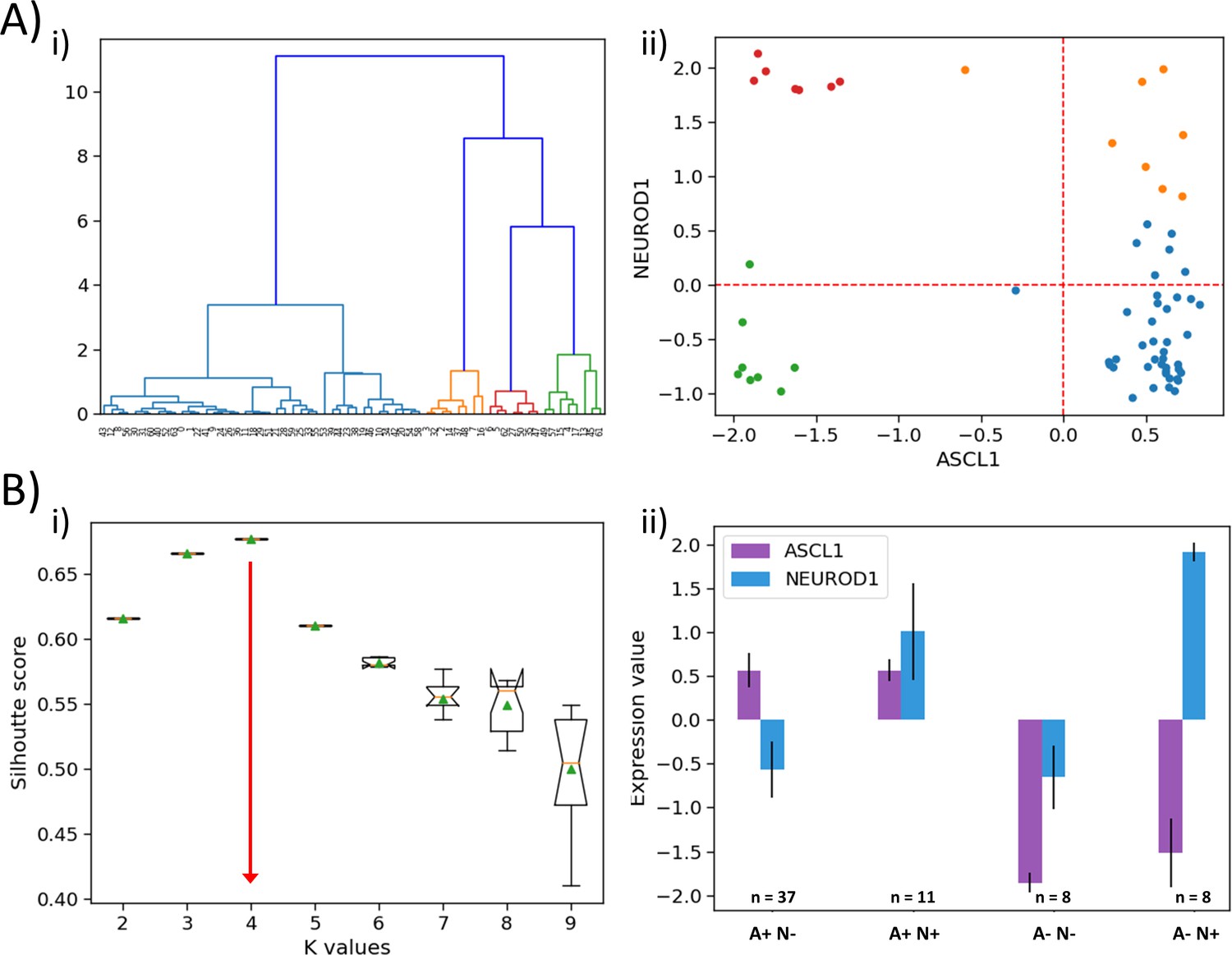
Analysis for GSE73160 using ASCL1 and NEUROD1.
(A) (i) Hierarchical clustering of GSE73160 dataset across ASCL1 and NEUROD1. (ii) Scatter plot of normalized gene expression for NEUROD1 vs ASCL1 of GSE73160 dataset, labeled by n = 4 clusters obtained from the earlier dendrogram. (B) (i) Silhouette score analysis across ASCL1 and NEUROD1 for the GSE73160 dataset. (ii) Expression levels ASCL1 and NEUROD1 in four clusters obtained from the GSE73160 dataset by k-means clustering.
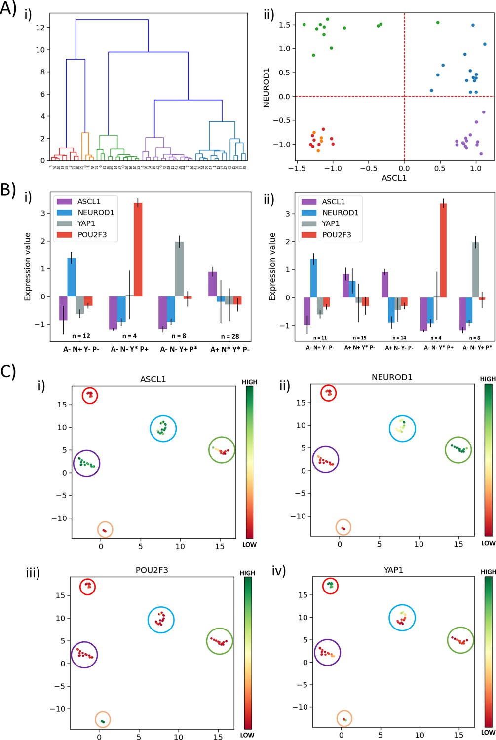
Figure 4—figure supplement 2
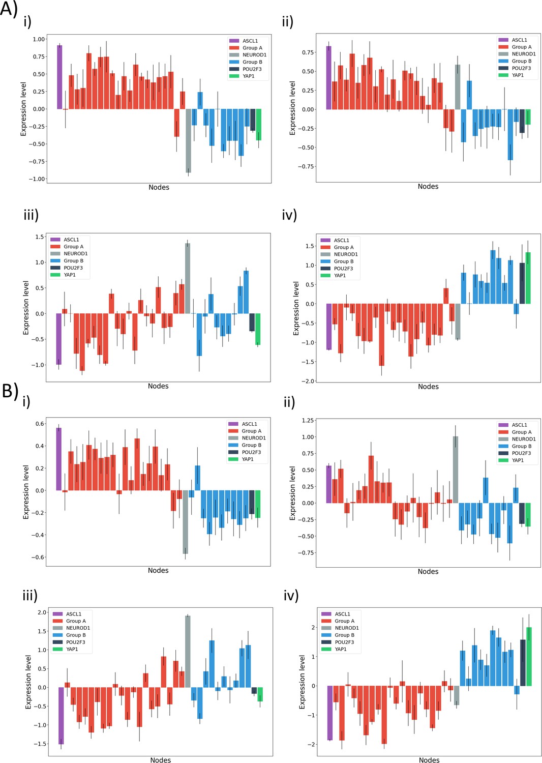
Gene expression of nodes involved in graph after clustering: Red bars indicate a node belonging to group A, and blue bar indicates belonging to group B.
ASCL1, NEUROD1, YAP1, and POU2F3 have different colors for better comparison (A) (i–iv) Hierarchical clustering of CCLE dataset across ASCL1 and NEUROD1, with individual panels depicting individual clusters: (i) A+/N−, (ii) A+/N+, (iii) A−/N+, (iv) A−/N−. and (B) (i–iv) K-means clustering of GSE73160 dataset ASCL1 and NEUROD1, with individual panels depicting individual clusters: (i) A+/N−, (ii) A+/N+, (iii) A−/N+, (iv) A−/N−.
Figure 4—figure supplement 3
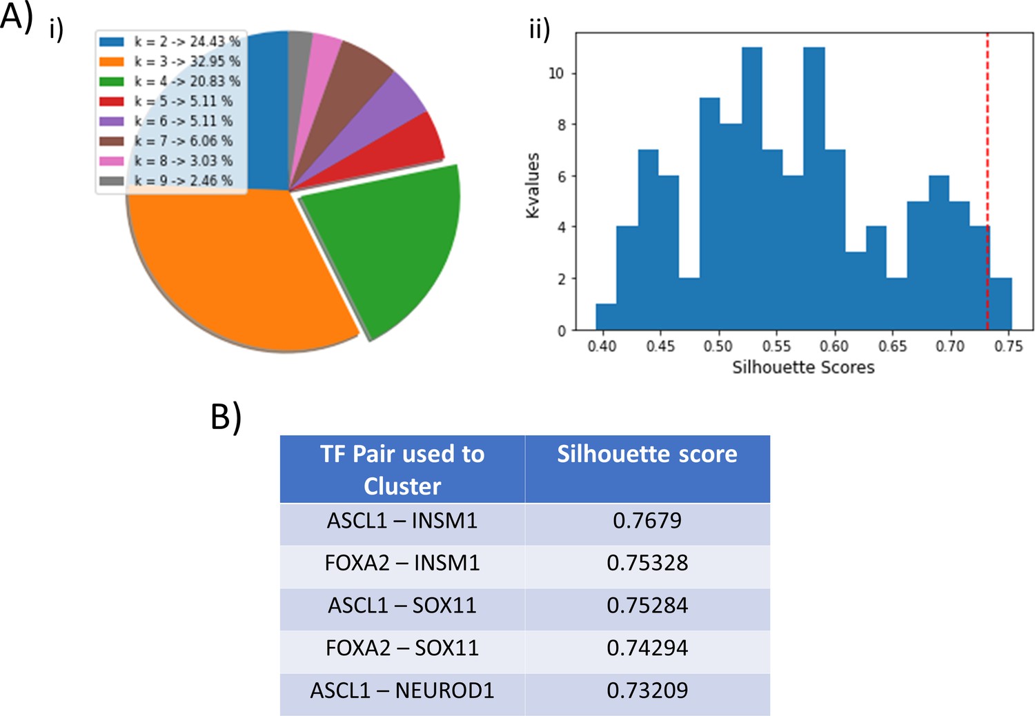
Clustering efficiency of other node pairs.
(A) (i) Pie-chart depicting the frequency of cases for different optimal k-values, as identified by average silhouette score analysis, for all combinations of two nodes taken at a time (33C2). (ii) Histogram depicting the distribution of average silhouette scores for k = 4 clusters (red dotted line indicates silhouette score for ASCL1-NEUROD1 based clustering). (B) Top five gene pairs with maximum silhouette scores, for k = 4 as the optimal cluster value.
Figure 5 with 1 supplement
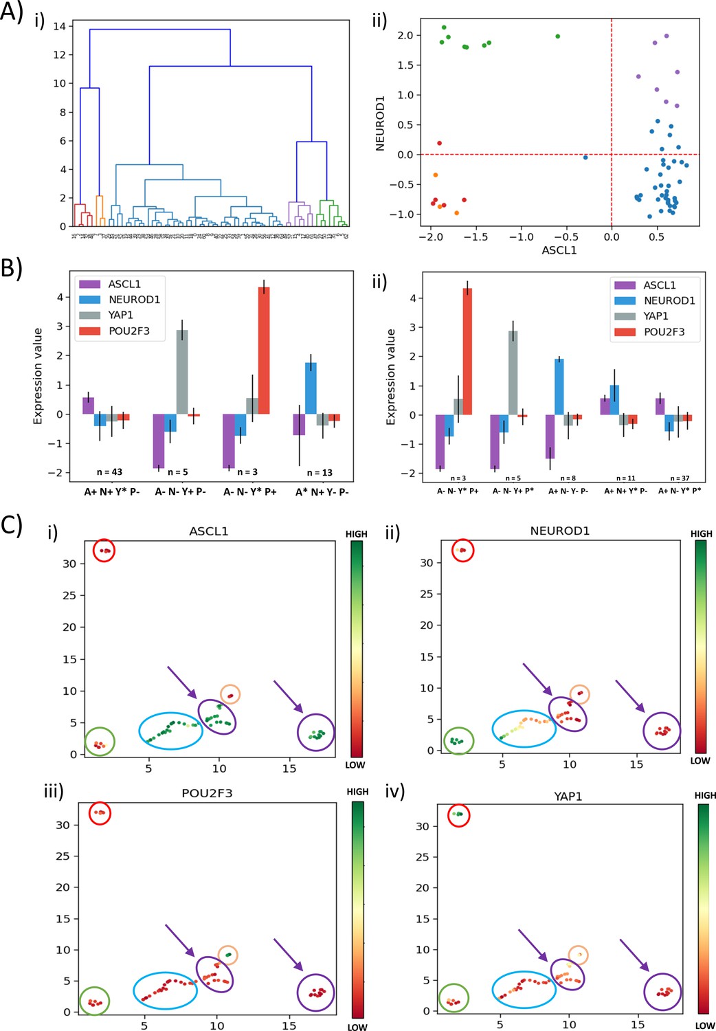
Classification of SCLC phenotypes based on ASCL1, NEUROD1, YAP1, and POU2F3.
(A) (i) Hierarchical clustering of CCLE samples using ASCL1, NEUROD1, YAP1, and POU2F3. (ii) Scatter plot of normalized gene expression data for CCLE samples for NEUROD1 and ASCL1. Color coding in dendrogram and scatter plot are synonymous (i.e. refer to the same cluster). (B) (i) Average levels of expression values for ASCL1, NEUROD1, YAP1, and POU2F3 for the four clusters identified in CCLE SCLC cell lines for K = 4. (ii) Same as (i) but for K = 5. (C) UMAP projections for CCLE dataset from four dimensions (ASCL1, NEUROD1, YAP1, and POU2F3) to two dimensions. Colorbar shows individual expression levels of ASCL1, NEUROD1, POU2F3, and YAP1. Color of the enclosing circle follows the same scheme as that for dendrogram and scatter plot.
Figure 5—figure supplement 1
Analysis for GSE73160 using ASCL1, NEUROD1, POU2F3, and YAP1.
(A) (i) Hierarchical clustering of GSE73160 dataset across ASCL1, NEUROD1, YAP1, and NPOU2F3. (ii) Scatter plot of normalized gene expression for NEUROD1 vs ASCL1 of GSE73160 dataset, labeled by n = 5 clusters obtained from the earlier dendrogram. (B) (i) Expression levels of four classifying genes (ASCL1, NEUROD1, YAP1, and POU2F3) in clusters obtained from the k-means algorithm for k = 4 in the GSE73160 dataset. (ii) Same as (i) but for k = 5. (C) (i–iv) UMAP projection of GSE73160 dataset from four dimensions (ASCL1, NEUROD1, YAP1, and POU2F3) to two dimensions. The labeling is based on expression levels of ASCL1 (i), NEUROD1 (ii), POU2F3 (iii), and YAP1 (iv).
Additional files
-
Supplementary file 1
Frequency distributions for SCLC network.
(a) Frequency distribution for asynchronous Boolean update of WT SCLC network using Ising update with 220 and 225 initial conditions over three replicates. (b) Steady-state frequency distribution for top 20 states of binarized RACIPE simulation of the network. (c) Node summary of single-edge perturbation of wild-type SCLC network.
- https://cdn.elifesciences.org/articles/64522/elife-64522-supp1-v2.xlsx
-
Supplementary file 2
Cell line classification using ASCL1, NEUROD1, YAP1 and POU2F3.
(a) Cell line classification of CCLE dataset using different cluster values for k-means and hierarchical algorithm over four genes of interest (ASCL1, NEUROD1, YAP1, and POU2F3). Also contains the classification as given by Wooten et al., 2019. (b) Cell line classification of GSE73160 dataset using different cluster values for k-means and hierarchical algorithm over four genes of interest (ASCL1, NEUROD1, YAP1, and POU2F3). Also contains the classification as given by Wooten et al., 2019 (for the cell lines included in both GSE73160 and CCLE).
- https://cdn.elifesciences.org/articles/64522/elife-64522-supp2-v2.xlsx
-
Supplementary file 3
Frequency distributions for reduced SCLC network.
(a) Steady-state frequency distribution for asynchronous Boolean update of network for genes corresponding to GROUP A and ELF3. (b) Steady-state frequency distribution for asynchronous Boolean update of network for genes corresponding to GROUP A only. (c) Steady-state frequency distribution for asynchronous Boolean update of network for genes corresponding to GROUP B only. (b) Steady-state frequency distribution for asynchronous Boolean update of network for genes corresponding to GROUP A only. Steady-state frequency distribution for asynchronous Boolean update of network for genes corresponding to GROUP B only. Steady-state frequency distribution for asynchronous Boolean update of network for genes corresponding to GROUP B and ELF3.
- https://cdn.elifesciences.org/articles/64522/elife-64522-supp3-v2.xlsx
-
Transparent reporting form
- https://cdn.elifesciences.org/articles/64522/elife-64522-transrepform-v2.docx
Download links
A two-part list of links to download the article, or parts of the article, in various formats.
Downloads (link to download the article as PDF)
Open citations (links to open the citations from this article in various online reference manager services)
Cite this article (links to download the citations from this article in formats compatible with various reference manager tools)
Topological signatures in regulatory network enable phenotypic heterogeneity in small cell lung cancer
eLife 10:e64522.
https://doi.org/10.7554/eLife.64522


