Figures and data in Modelling the neural code in large populations of correlated neurons

Figures
Tables
Additional files

10 figures, 3 tables and 1 additional file

Figures

Figure 1

Download asset Open asset

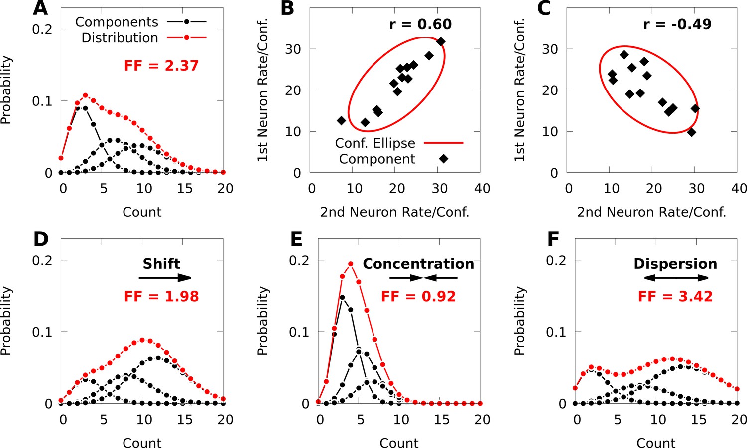
Poisson mixtures and Conway-Maxwell extensions exhibit spike-count correlations, and over- and under-disperson.

(A) A Poisson mixture distribution (red), defined as the weighted sum of three component Poisson distributions (black; scaled by their weights). FF denotes the Fano Factor (variance over mean) of the mixture. (B, C) The average spike-count (rate) of the first and second neurons for each of 13 components (black dots) of a bivariate IP mixture, and 68% confidence ellipses for the spike-count covariance of the mixture (red lines; see Equations 6 and 7). The spike-count correlation of each mixture is denoted by $r$ . (D) Same model as A, except we shift the distribution by increasing the baseline rate of the components. (E, F) Same model as A, except we use an additional baseline parameter based on Conway-Maxwell Poisson distributions to concentrate (E) or disperse (F) the mixture distribution and its components.

Figure 2

Download asset Open asset

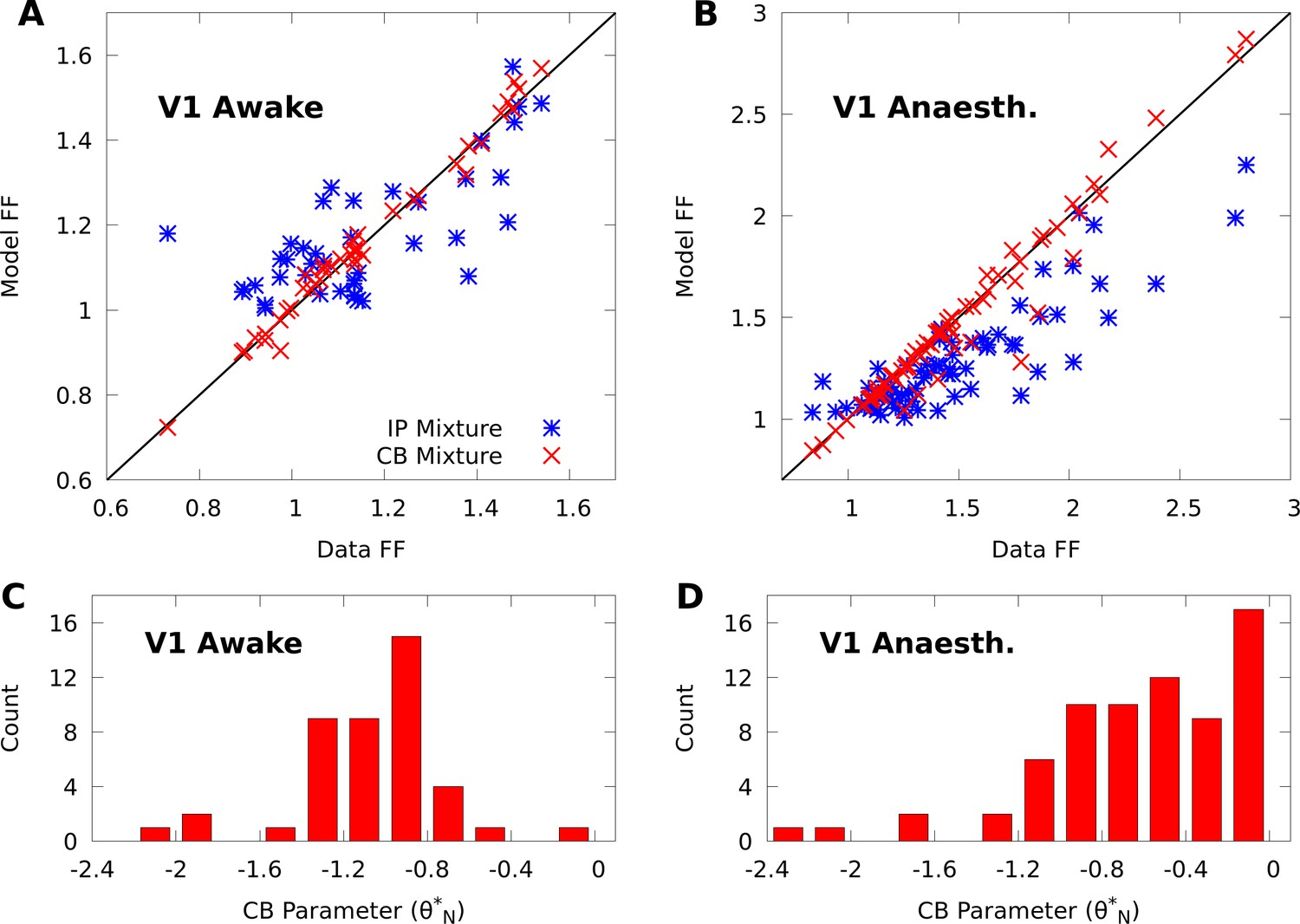
CoM-based parameters help Poisson mixtures capture individual variability in V1 responses to a single stimulus.

We compare Independent Poisson (IP) mixtures (Equation 1) and CoM-Based (CB) mixtures (Equation 2) on neural population responses to stimulus orientation $x = 20^{\circ}$ in V1 of awake ( $d_{N} = 43$ neurons and $d_{T} = 355$ trials) and anaesthetized ( $d_{N} = 70$ and $d_{T} = 1, 200$ ) macaques; both mixtures are defined with $d_{K} = 5$ components for both data sets (see Materials and methods for training algorithms). **A,B:** Empirical Fano factors of the awake (A) and anaesthetized data (B), comparing IP (blue) and CB mixtures (red). **C,D:** Histogram of the CB parameters $θ_{N}^{*}$ for the CB mixture fits to the awake (C) and anaesthetized (D) data. Values of $θ_{N}^{*} < - 1$ denote under-dispersed mixture components, values $> - 1$ denote over-dispersed components.

Figure 3

Download asset Open asset

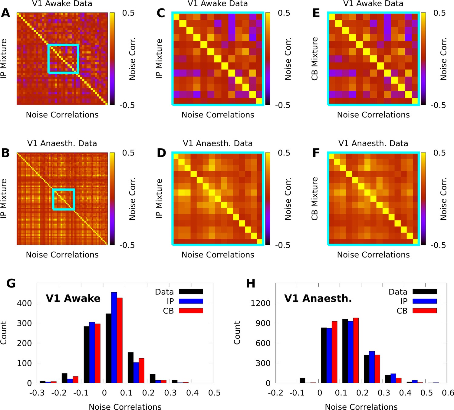
IP and CB mixtures effectively capture pairwise covariability in V1 responses to a single stimulus.

Here we analyze the pairwise statistics of the same models from Figure 2. (**A, B**) Empirical correlation matrix (upper right triangles) of awake (A) and anaesthetized data (B), compared to the correlation matrix of the corresponding IP mixtures (lower left triangles). (C, D) Noise correlations highlighted in A and B, respectively. (E, F) Highlighted noise correlations for CB mixture fit. (G,H) Histogram of empirical noise correlations, and model correlations from IP and CB mixtures.

Figure 4

Download asset Open asset

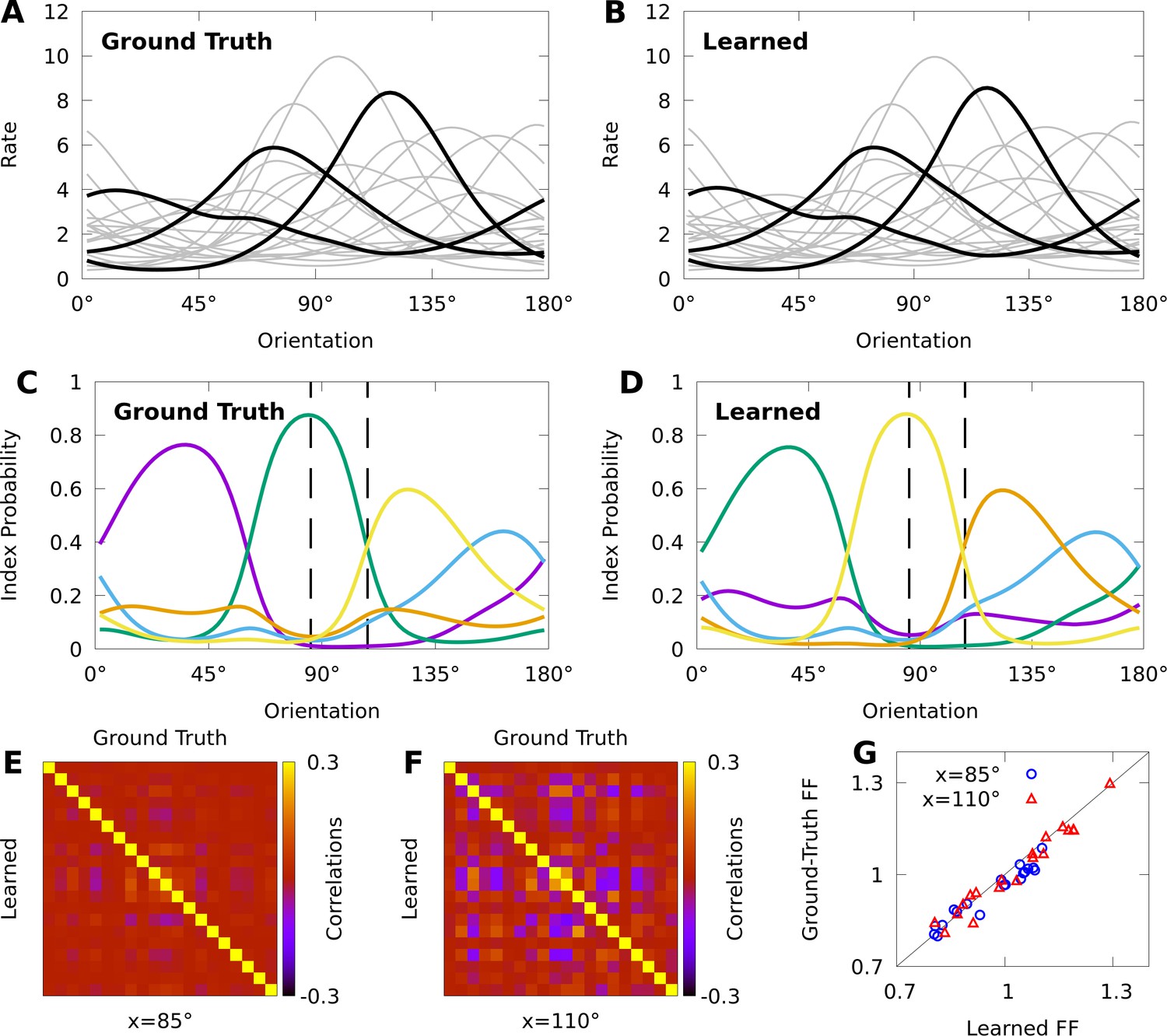
Expectation-maximization recovers a ground truth CoM-based, conditional mixture (CB-CM).

We compare a ground truth, CB-CM with 20 neurons, five mixture components, von Mises-tuned components, and randomized parameters to a learned CB-CM fit to 2000 samples from the ground truth CB-CM. **A,B:** Tuning curves of the ground-truth CB-CM (A) and learned CB-CM (B). Three tuning curves are highlighted for effect. **C,D:** The orientation-dependent index probabilities of the ground truth CB-CM (C) and learned CB-CM (D), where colour indicates component index. Dashed lines indicate example stimulus-orientations used in E, F, and G. (E, F) The correlation matrix of the ground truth CB-CM (upper right), compared to the correlation matrix of the learned CB-CM (lower left) at stimulus orientations $x = 85^{\circ}$ (E) and $x = 110^{\circ}$ (F). (G) The FFs of the ground-truth CB-CM compared to the learned CB-CM at orientations $x = 85^{\circ}$ (blue circles) and $x = 110^{\circ}$ (red triangles).

Figure 5

Download asset Open asset

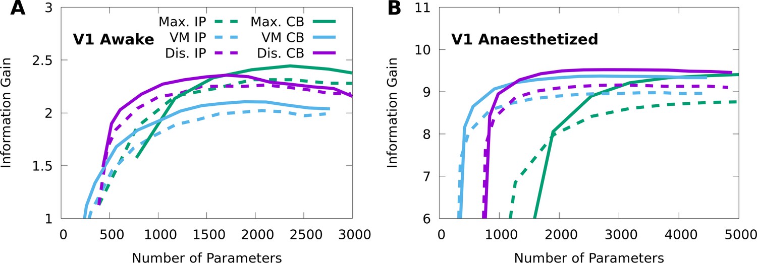
Finding the optimal number of parameters for CMs to model neural responses in macaque V1.

10-fold cross-validation of the information gain given awake V1 data (A) and anaesthetized V1 data (B), as a function of the number of model parameters, for multiple forms of CM: maximal CMs (green); minimal CMs with von Mises component tuning (blue); minimal CMs with discrete component tuning (purple); and for each case we consider either IP (dashed lines) or CB (solid lines) variants. Standard errors of the information gain are not depicted to avoid visual clutter, however they are approximately independent of the number of model parameters, and match the values indicated in Table 2.

Figure 6

Download asset Open asset

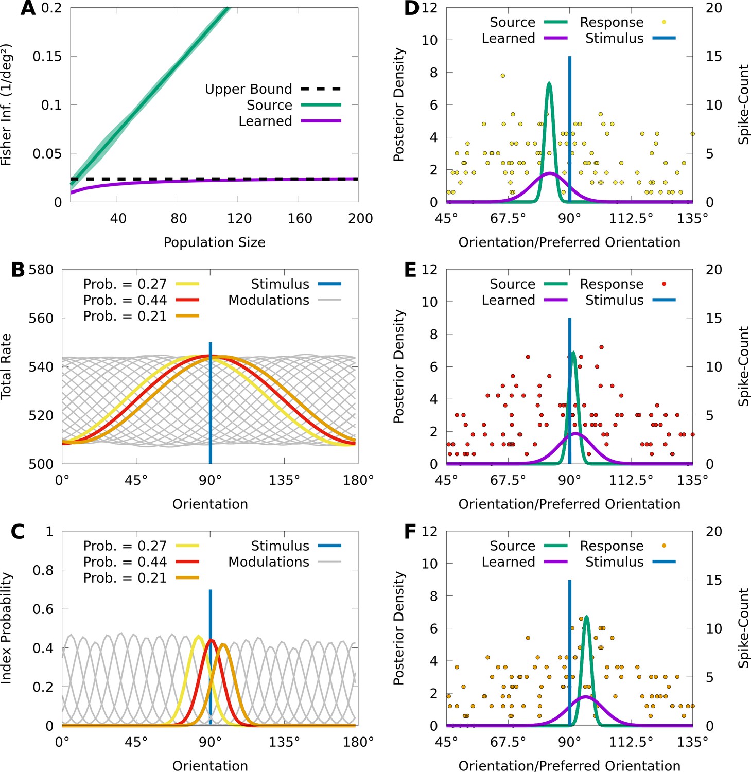
CMs can capture information-limiting correlations in data.

We consider a von Mises-tuned, independent Poisson source model (green) with $d_{K} = 200$ neurons, and an information-limited, IP-CM (purple) with $d_{K} = 25$ components, fit to 10,000 responses of the source-model to stimuli obscured by von Mises noise. In **B-F** we consider a stimulus-orientation $x = 90^{\circ}$ (blue line). (A) The average (lines) and standard deviation (filled area) of the FI over orientations, for the source (green) and information-limited (purple) models, as a function of random subpopulations, starting with ten neurons, and gradually reintroducing missing neurons. Dashed black line indicates the theoretical upper bound. (B) The sum of the firing rates of the modulated IP-CM for all indices $k > 1$ (lines) as a function of orientation, with three modulated IP-CMs highlighted (red, yellow, and orange lines) corresponding to the highlighted indices in C. (C) The index-probability curves (lines) of the IP-CM for indices $k > 1$ and the intersection (red, yellow, and orange circles) of the stimulus with three curves (orange, yellow, and orange lines). (**D-F**) Three responses from the yellow (D; yellow points), red (E; red points), and orange modulated IP-CMs (F; orange points) indicated in C. For each response we plot the posterior based on the source model (green line) and the information-limited model (purple line).

Appendix 1—figure 1

Download asset Open asset

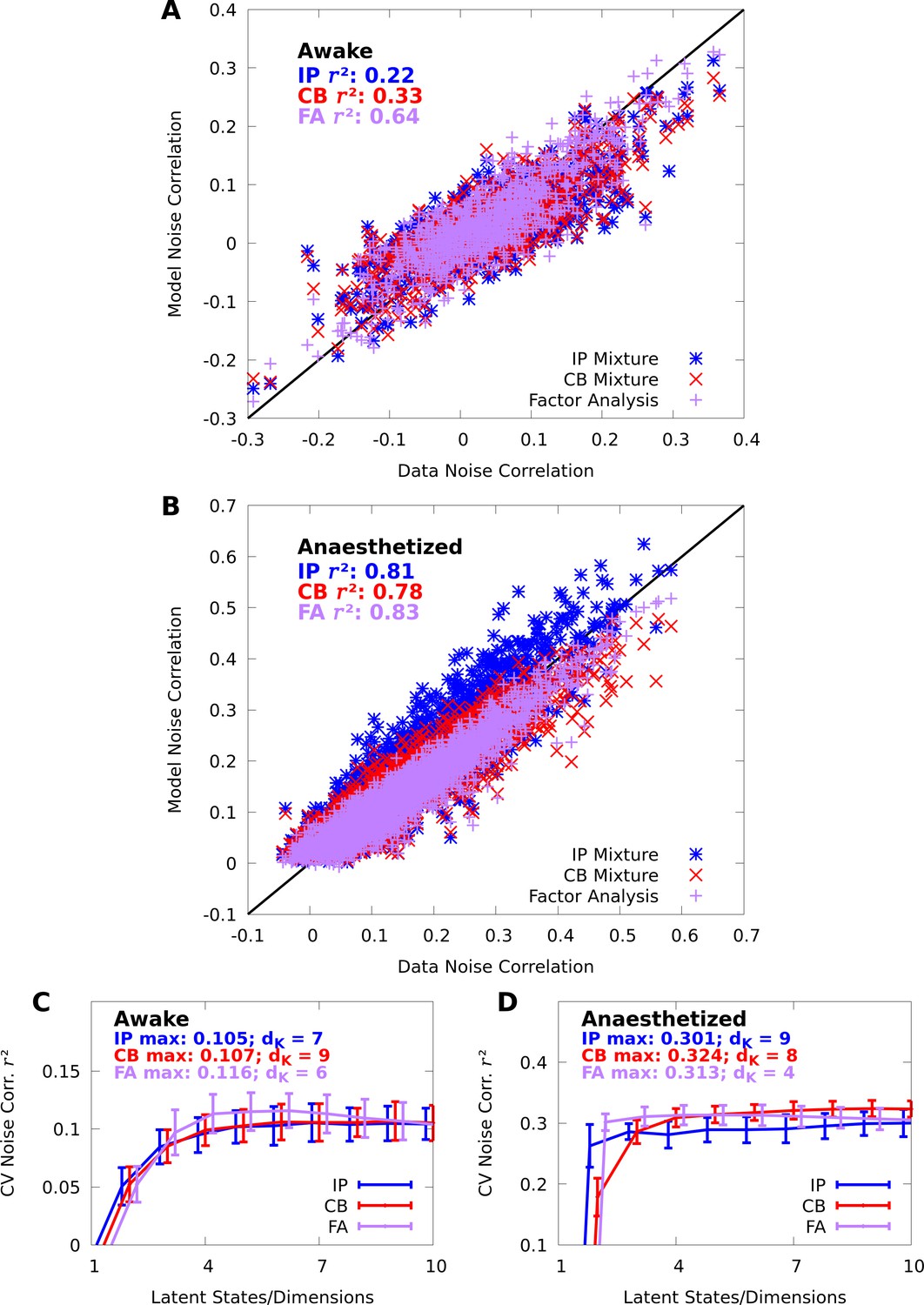
Mixture models capture spike-count correlations.

(A, B) Scatter plots of the data noise correlations versus the noise correlations modelled by IP (blue) and CB (red) mixtures, and FA (purple), in both the awake (A) and anaesthetized (B) datasets at orientation $x = 40^{\circ}$ . Each point represent a pair of neurons ( $d_{N} = 43$ and $d_{N} = 70$ neurons in the awake and anaesthetized datasets, respectively). (C, D) We evaluate the noise correlation $r^{2}$ over all stimulus-orientations with 10-fold cross-validation. We plot the average (lines) and standard error (error bars) of the cross-validated noise correlation $r^{2}$ as a function of number of latent states/dimensions $d_{K}$ , in both the awake (C) and anaesthetized (D) datasets. We also indicate the peak performance achieved for each model, and requisite number of latent states/dimensions $d_{K}$ .

Appendix 1—figure 2

Download asset Open asset

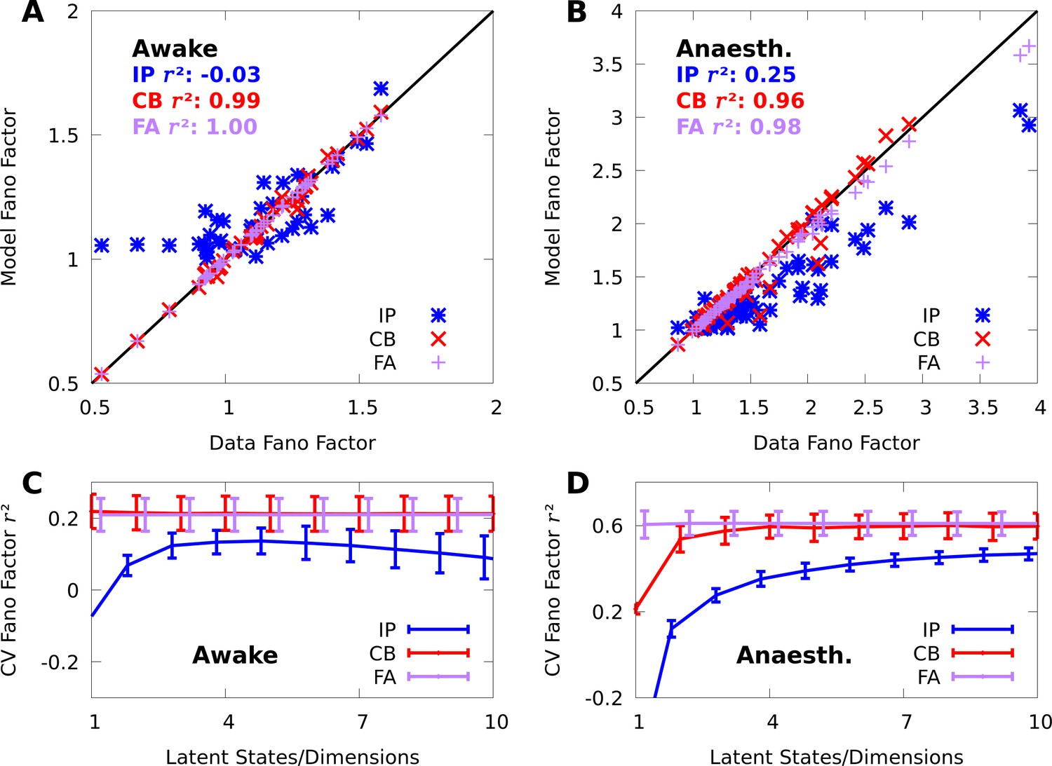
Mixture models capture spike-count Fano factors.

We repeat the analyses from Appendix References Figure 7 on Fano factors (FFs). (A, B) Scatter plots of the data FFs versus the FFs modelled by IP (blue) and CB mixtures (red), and FA (purple) in both the awake (A) and anaesthetized (B) datasets at orientation $x = 40^{\circ}$ . (C, D) As a function of the number of latent states/dimensions, we plot the average (lines) and standard error (bars) of the cross-validated $r^{2}$ between the data and modelled Fano factors over all stimulus orientations, in both the awake (C) and anaesthetized (D) datasets.

Appendix 2—figure 1

Download asset Open asset

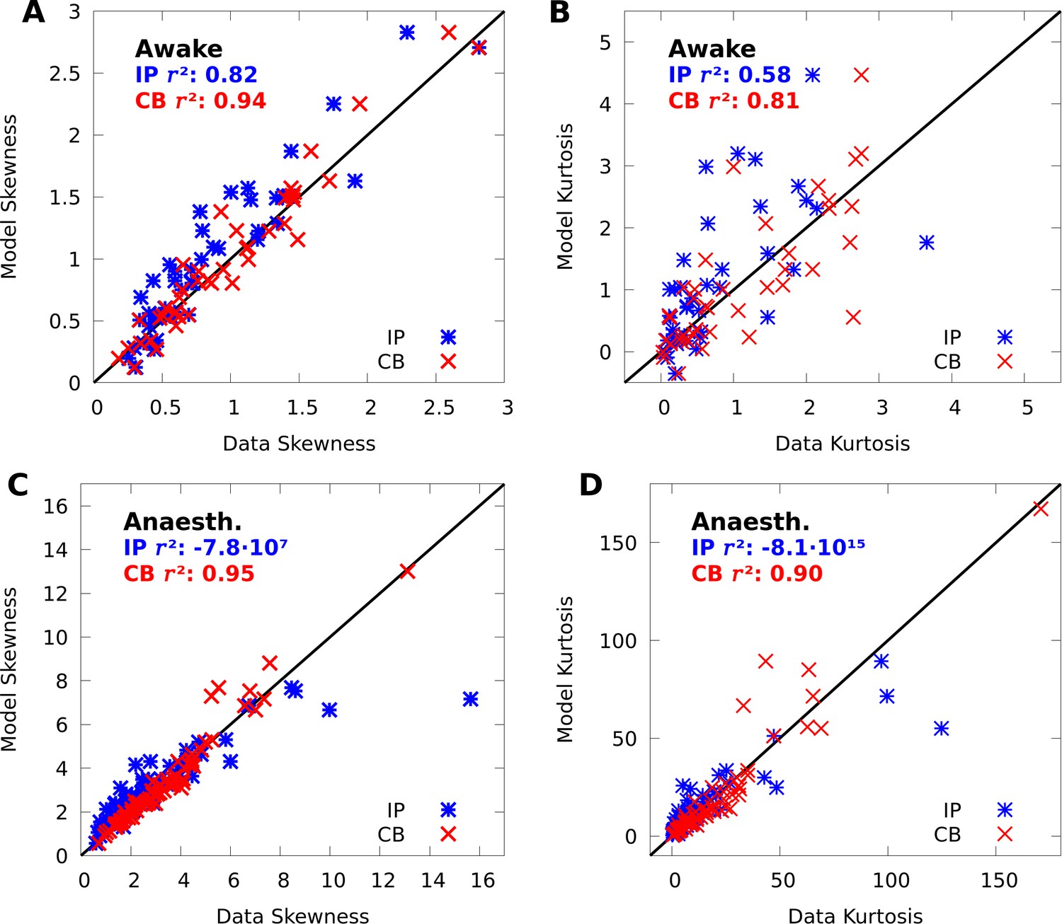
CoM-based mixtures capture data skewness and kurtosis.

(A, B) Scatter plots of the data skewness (A) and kurtosis (B) versus the skewness and kurtosis modelled by IP mixtures (blue) and CB mixtures (red). The skewness and kurtosis of 1 of 43 neurons modelled by the IP mixture were outside the bounds of each scatter plot. C,D: Same as A-B but on the anaesthetized data; the skewness of 11 of 43, and kurtosis of 12 of 43 neurons modelled by the IP mixture were outside the bounds of each scatter plot.

Appendix 3—figure 1

Download asset Open asset

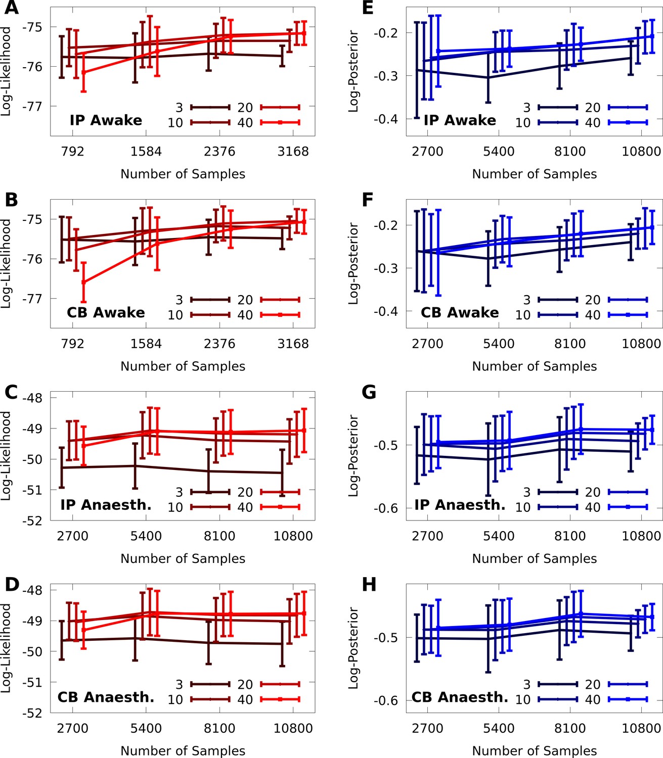
Sample complexity of discrete CMs.

10-fold cross-validation of discrete CMs with 3, 10, 20, and 40 components, on subsamples of 25%, 50%, 75%, and 100% of the awake and anaesthetized datasets, with $d_{N} = 43$ and $d_{N} = 50$ neurons, respectively. *Left column*: Cross-validated average log-likelihood of the models given test data (i.e. encoding performance). *Right column*: Cross-validated average log-posterior (i.e. decoding performance). Error bars represent standard error. In all panels, we added an offset on the abscissa for better visualization of the error bars.

Tables

Table 1

Parameter counts of CM models.

First row is number of parameters in IP models, second row is number of additional parameters in CB extensions of IP models, as a function of number of stimuli $d_{S}$ , neurons $d_{N}$ , and mixture components $d_{K}$ .

Model parameter formulae
	Maximal	Von mises	Discrete
Num. Params	$d_{S} (d_{N} d_{K} + d_{K} - 1)$	$(d_{N} + 1) (d_{K} - 1) + 3 d_{N}$	$(d_{N} + 1) (d_{K} - 1) + d_{S} d_{N}$
Add. CB Params	$d_{S} d_{N}$	$d_{N}$	$d_{N}$

Table 2

Conditional mixtures models of neural responses in macaque V1 capture significant information about higher-order statistics.

We apply 10-fold cross-validation to estimate the mean and standard error of the information gain (model log-likelihood -log-likelihood of a non-mixed, independent Poisson model in nats/trial) on held-out data, from either awake (sample size $d_{T} = 3, 168$ , from $d_{N} = 43$ neurons, over $d_{S} = 9$ orientations) or anaesthetized ( $d_{T} = 10, 800$ , $d_{N} = 70$ , $d_{S} = 9$ ) macaque V1. We compare maximal CMs, minimal CMs with von Mises-tuned components, and minimal CMs with discrete-tuned components, and for each case we consider either IP or CB variants. For each variant, we indicate the number of CM components $d_{K}$ and the corresponding number of model parameters required to achieve peak information gain (cross-validated). For reference, the non-mixed, independent Poisson models use 129 and 210 parameters for the awake and anaesthetized data, respectively.

Encoding performance
	V1 awake data			V1 anaesthetized data
CM Variant	Inf. Gain ( $\frac{Nats}{Trial}$ )	$d_{K}$	# Params.	Inf. Gain ( $\frac{Nats}{Trial}$ )	$d_{K}$	# Params.
Maximal IP	$2.30 \pm 0.32$	5	1971	$8.77 \pm 0.71$	8	5103
Maximal CB	$2.44 \pm 0.35$	5	2358	$9.42 \pm 0.70$	7	5094
Von Mises IP	$2.01 \pm 0.26$	45	2065	$8.97 \pm 0.70$	40	2979
Von Mises CB	$2.10 \pm 0.25$	40	1888	$9.38 \pm 0.69$	35	2694
Discrete IP	$2.25 \pm 0.28$	40	2103	$9.17 \pm 0.70$	35	3044
Discrete CB	$2.35 \pm 0.29$	30	1706	$9.53 \pm 0.68$	30	2689
Non-mixed IP	0	1	129	0	1	210

Table 3

CMs support high-performance decoding of neural responses in macaque V1.

We apply 10-fold cross-validation to estimate the mean and standard error of the average log-posteriors $\log p (x ∣ 𝐧)$ on held-out data, from either awake or anaesthetized macaque V1. We compare discrete, minimal, CB-CM (CB-CM) and IP-CM (IP-CM); an independent Poisson model with discrete tuning (Non-mixed IP); a multiclass linear decoder (Linear); and a multiclass nonlinear decoder defined as an artificial neural network with two hidden layers (Artificial NN). The number of CM components $d_{K}$ was chosen to achieve peak information gain in Figure 5. The number of ANN hidden units was chosen based on peak cross-validation performance. In all cases we also indicate the number of model parameters required to achieve the indicated performance.

Decoding performance
	V1 awake data		V1 anaesthetized data
	Average Log-Post.	Num. Params.	Average Log-Post.	Num. Params.
IP-CM	$- 0.207 \pm 0.039$	2103	$- 0.448 \pm 0.026$	3044
CB-CM	$- 0.206 \pm 0.043$	1706	$- 0.441 \pm 0.023$	2689
Non-mixed IP	$- 0.272 \pm 0.067$	387	$- 0.967 \pm 0.071$	630
Linear	$- 0.256 \pm 0.053$	352	$- 0.457 \pm 0.019$	568
Artificial NN	$- 0.200 \pm 0.032$	527,108	$- 0.426 \pm 0.015$	408,008

Additional files

Transparent reporting form: https://cdn.elifesciences.org/articles/64615/elife-64615-transrepform-v2.docx
Download elife-64615-transrepform-v2.docx

Download links

A two-part list of links to download the article, or parts of the article, in various formats.

Downloads (link to download the article as PDF)

Article PDF

Open citations (links to open the citations from this article in various online reference manager services)

Mendeley

Cite this article (links to download the citations from this article in formats compatible with various reference manager tools)

Sacha Sokoloski
Amir Aschner
Ruben Coen-Cagli

(2021)

Modelling the neural code in large populations of correlated neurons

eLife 10:e64615.

https://doi.org/10.7554/eLife.64615

Share this article

Cite this article

Poisson mixtures and Conway-Maxwell extensions exhibit spike-count correlations, and over- and under-disperson.

CoM-based parameters help Poisson mixtures capture individual variability in V1 responses to a single stimulus.

IP and CB mixtures effectively capture pairwise covariability in V1 responses to a single stimulus.

Expectation-maximization recovers a ground truth CoM-based, conditional mixture (CB-CM).

Finding the optimal number of parameters for CMs to model neural responses in macaque V1.

CMs can capture information-limiting correlations in data.

Mixture models capture spike-count correlations.

Mixture models capture spike-count Fano factors.

CoM-based mixtures capture data skewness and kurtosis.

Sample complexity of discrete CMs.

Parameter counts of CM models.

Conditional mixtures models of neural responses in macaque V1 capture significant information about higher-order statistics.

CMs support high-performance decoding of neural responses in macaque V1.

Transparent reporting form

Downloads (link to download the article as PDF)

Open citations (links to open the citations from this article in various online reference manager services)

Cite this article (links to download the citations from this article in formats compatible with various reference manager tools)