Non-genetic inheritance restraint of cell-to-cell variation
- Department of Physics and Astronomy, The Dietrich School of Arts and Sciences, University of Pittsburgh, United States
- Department of Computational and Systems Biology, School of Medicine, University of Pittsburgh, United States
Figures
Figure 1 with 2 supplements
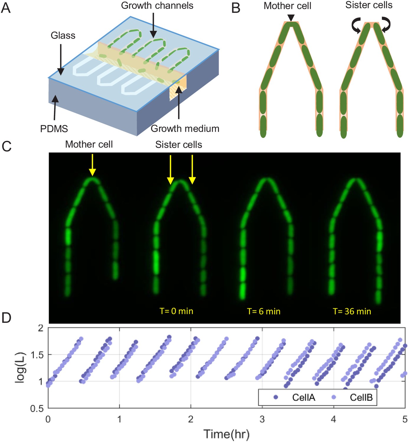
Scheme of the experimental setup for tracking sister cells.
(A) Long (30 μm) narrow traps (1 μm—1 μm) are connected on one end and open on the other to wide (30 μm—30 μm) perpendicular flow channels through which fresh medium is pumped and washes out cells that are pushed out of the traps. (B) Illustration of SCs being born from a single mother cell at the tip of the trap, as can also be seen in real fluorescence images of the cells in the trap (C), which are then followed for a long time (see Figure 1—video 1). (D) Section of example traces of two sister cells from the time they are born, which shows how they become different over time.
Figure 1—figure supplement 1
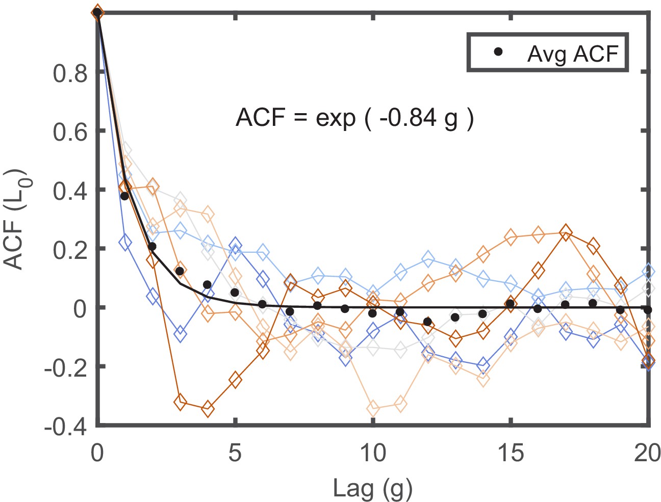
The ACFs of individual lineages measured in separate traps.
The ACFs of individual lineages, measured in the same experiment in separate traps in the mother machine, are presented in different colors. Each ACF was calculated from a lineage longer than 150 generations to maximize the statistics. Note that each ACF exhibits distinct dynamical pattern. Averaging all ACFs results in a simple exponentially decaying function with a decay time of ∼2 generations depicted by the black line in the graph.
Figure 1—video 1
Creation of sister cells (SCs) in the experimental setup.
Figure 2
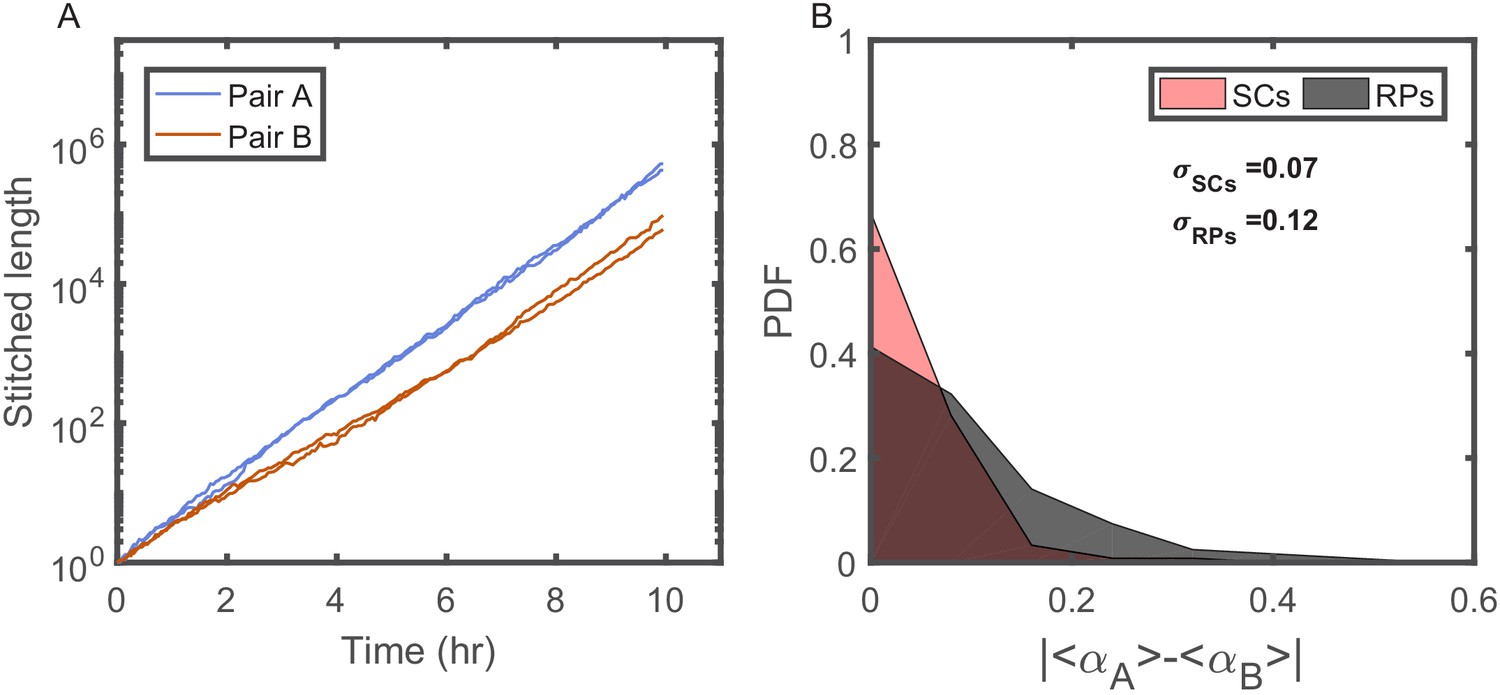
Individuality of cellular growth dynamics in different microenvironments.
(A) Depicts the cell length of two pairs of SCs measured in two different V-shaped traps as a function of time. The length of each cell is presented in a ‘stitched’ form, where the length of the cell in each cell cycle is adjusted to start from the length of the cell at the end of the previous cycle, ignoring by this the division events. This is done by dividing the length in each cycle by the starting length and multiplying it by the length of the cell at the end of the previous cycle. This presentation emphasizes the difference in the average growth rates measured in different traps. Note, however, that each pair of SCs exhibits similar average growth rate. (B) Probability distribution function (PDF) of the absolute difference in the average growth rate of two SCs is compared with the absolute difference in the average growth rate of two randomly paired cells (RPs) growing in separate traps in the same device (see Figure 4A for further elaboration on random pairing of cells). The standard deviation of the difference for SCs () is almost half of the calculated value for RPs (). This shows that cells grow with different average growth rates in different traps and supports the idea of micro-niche formation in the microfluidic device.
Figure 3
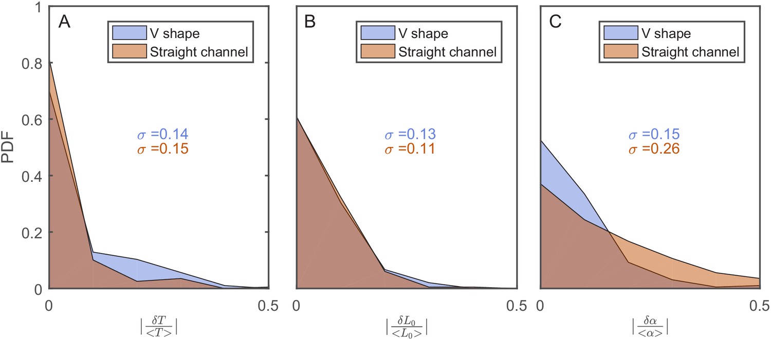
The effect of the v-shaped channel on the distribution of the different cellular characteristics between SCs during division.
(A) Probability distribution Function (PDF) of the difference in the first cell-cycle time of two sister cells after separation relative to the population’s average cycle time under the same experimental conditions. (B) PDF of the difference in cell length between the sister cells immediately after division relative to the population’s average length at the start of the cell cycle. (C) PDF of the difference in the growth rate of the two sister cells after separation relative to the population’s average growth rate. The difference measured in the straight channels here is larger than that measured in the v-shaped channels. This could be due to the fact that the two cells in the mother machine trap are at different distance from the nutrients diffusing from the flow channel into the traps. This has been shown before to result in variation in the cells growth rate (Yang et al., 2018). In all graphs, the blue curves represent the distributions measured in our new device with the v-shaped channels using 194 pairs, while the brown curves were measured in the straight channels of the mother machine using 198 pairs.
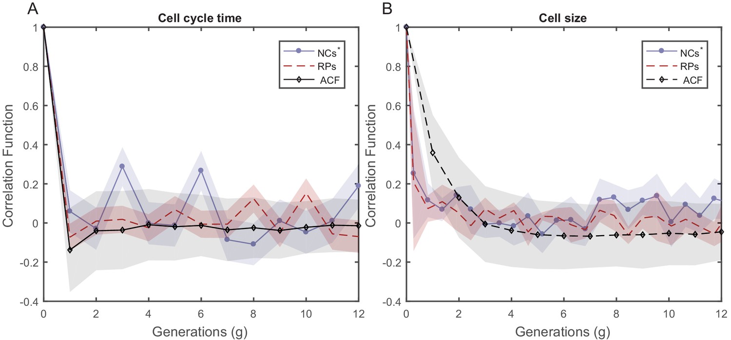
Figure 4 with 5 supplements
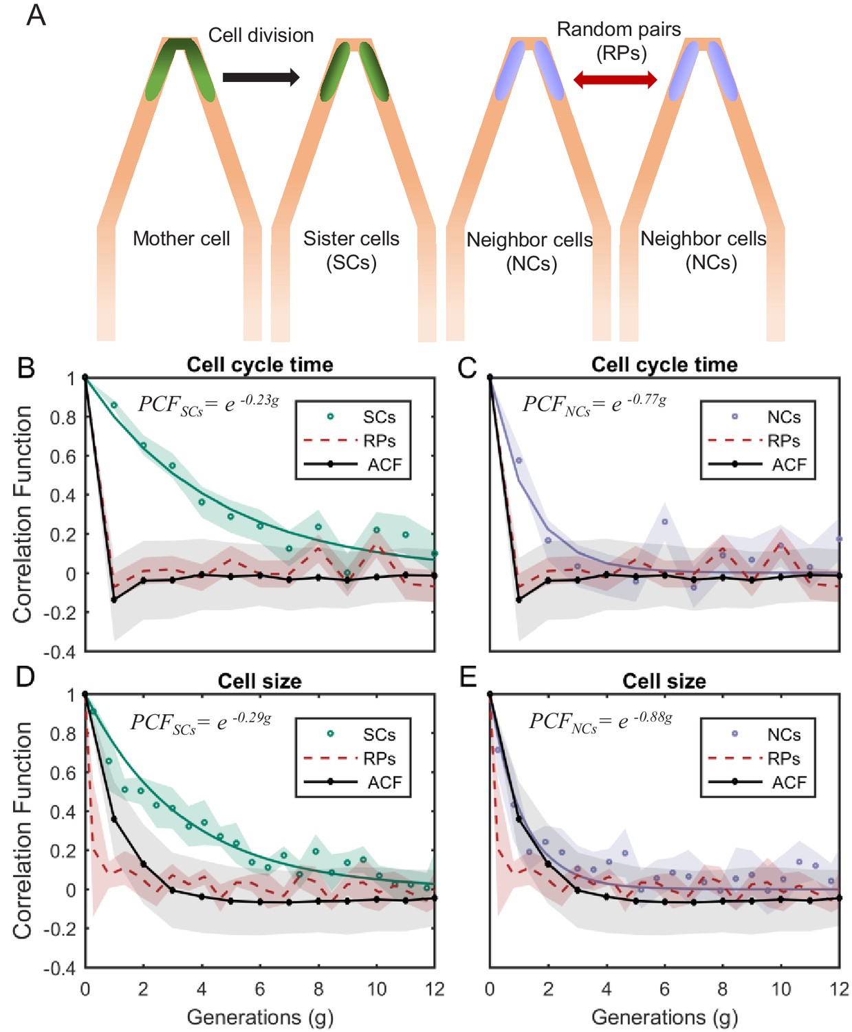
PCF of cell-cycle time and cell size measured in cell pairs as a function of number of generations.
(A) Three types of pairs used for calculating PCF. (B) PCF of cell-cycle time for SCs (122 pairs from three separate experiments) exhibit memory that extends for almost nine generations (half lifetime ∼ 4.5 generations). This is ∼3.5× longer than the half lifetime of NCs PCF (calculated using a 100 pairs from three separate experiments) (C), which is comparable to the ACF (half lifetime ∼1 generation). (D) Similarly, SCs exhibit strong cell size correlation that decays slowly over a long time (half lifetime ∼3.5 generations), while (E) NCs show almost no correlation in cell size similar to ACF of initial sizes (half lifetime ∼1 generation). For details of the cell-cycle time PCF and errors calculation see SI and Figure 4—figure supplements 1 and 2. PCF values for cell size were calculated in similar way to cell-cycle time and were then averaged over a window of six consecutive time frames (15 min time window) (See Figure 4—figure supplement 4 for raw data). Shaded area represents the standard deviation of the average. The equations in the graphs represent the best fit to the PCF depicted in each graph with g is generation number.
Figure 4—figure supplement 1
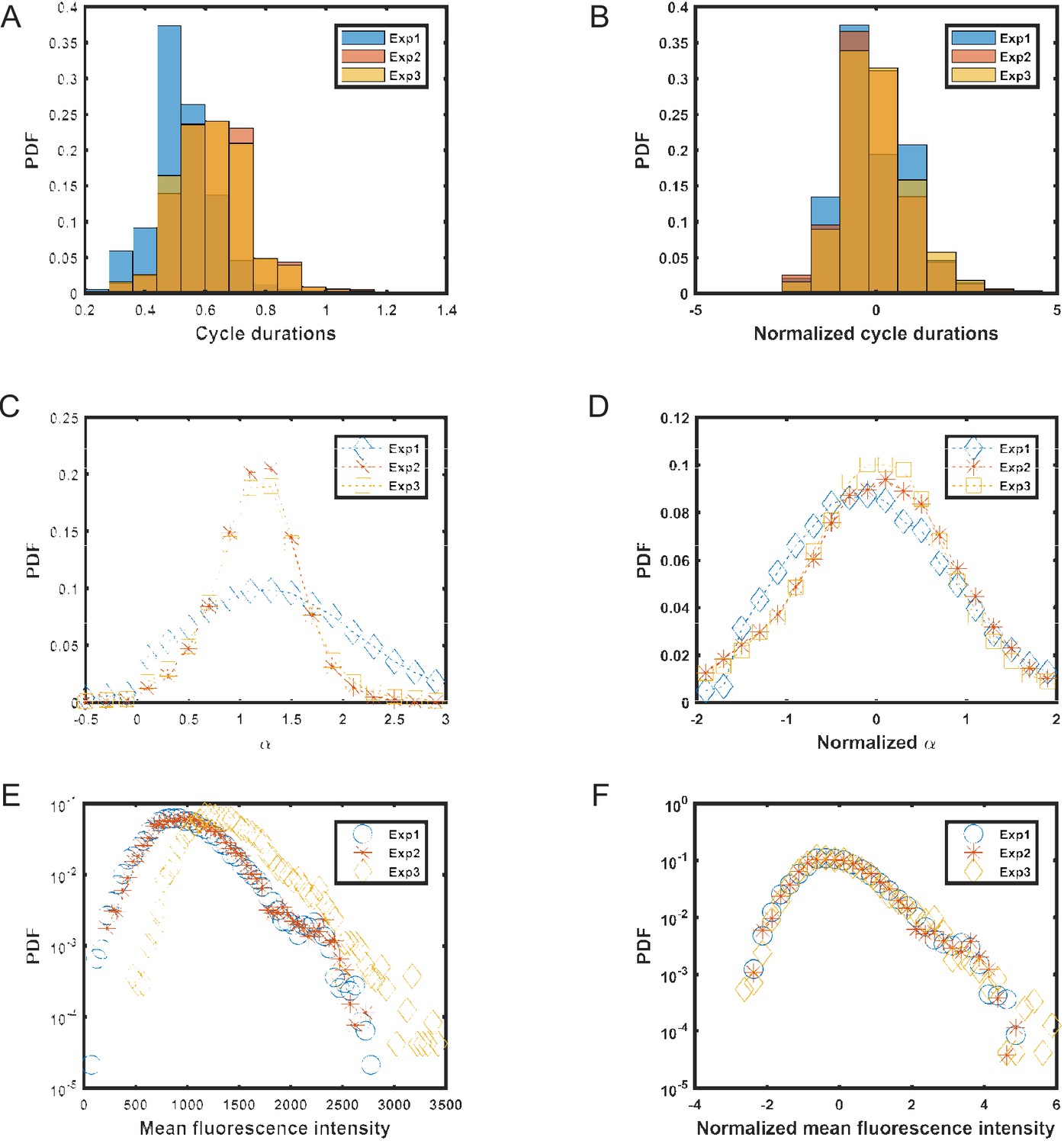
Distributions of different cell parameters.
In order to avoid artifacts arising in calculations due to differences between experiments carried out on different days, raw data from these experiments was normalized by subtracting the mean (μ) and dividing by the standard deviation (σ) for each experiment separately. Later, this normalized data was combined and used for calculating the PCF and variances for different parameters. (A,B) distributions of cell cycle times (T) before and after normalization. (C,D) distributions of elongation rate (α) before and after normalization. (E,F) distributions of mean fluorescence intensity (f) before and after normalization.
Figure 4—figure supplement 2
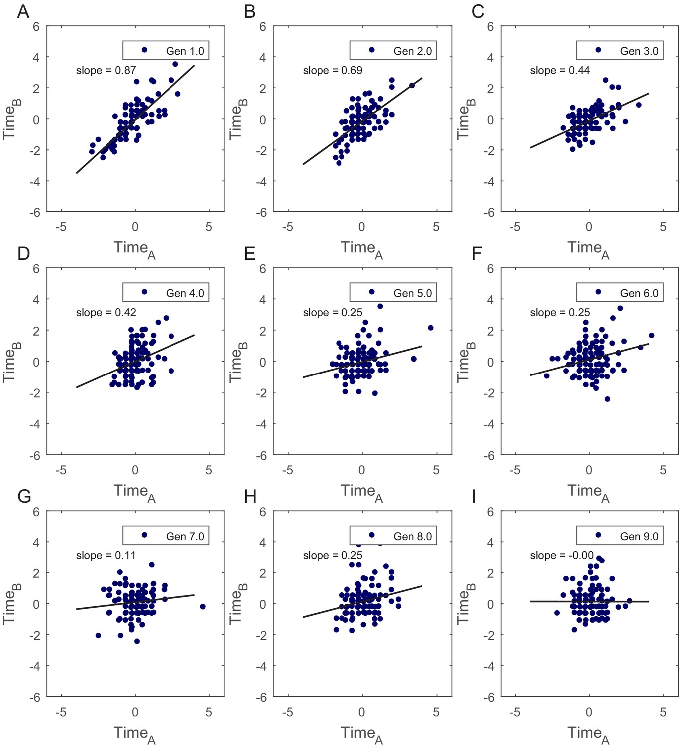
Correlation in cell-cycle times for SCs was verified by calculating slopes of best fits to the plots of normalized TimeA vs TimeB.
(A–I) Slopes of the best fit lines for TimeA vs TimeB show that cell-cycle times are strongly correlated for first few generations in SCs (summary of the slopes values is presented in Appendix 1—table 1). This shows existence of non-genetic memory that restrains the divergence of the phenotypes in cells originating from the same mother cell.
Figure 4—figure supplement 3
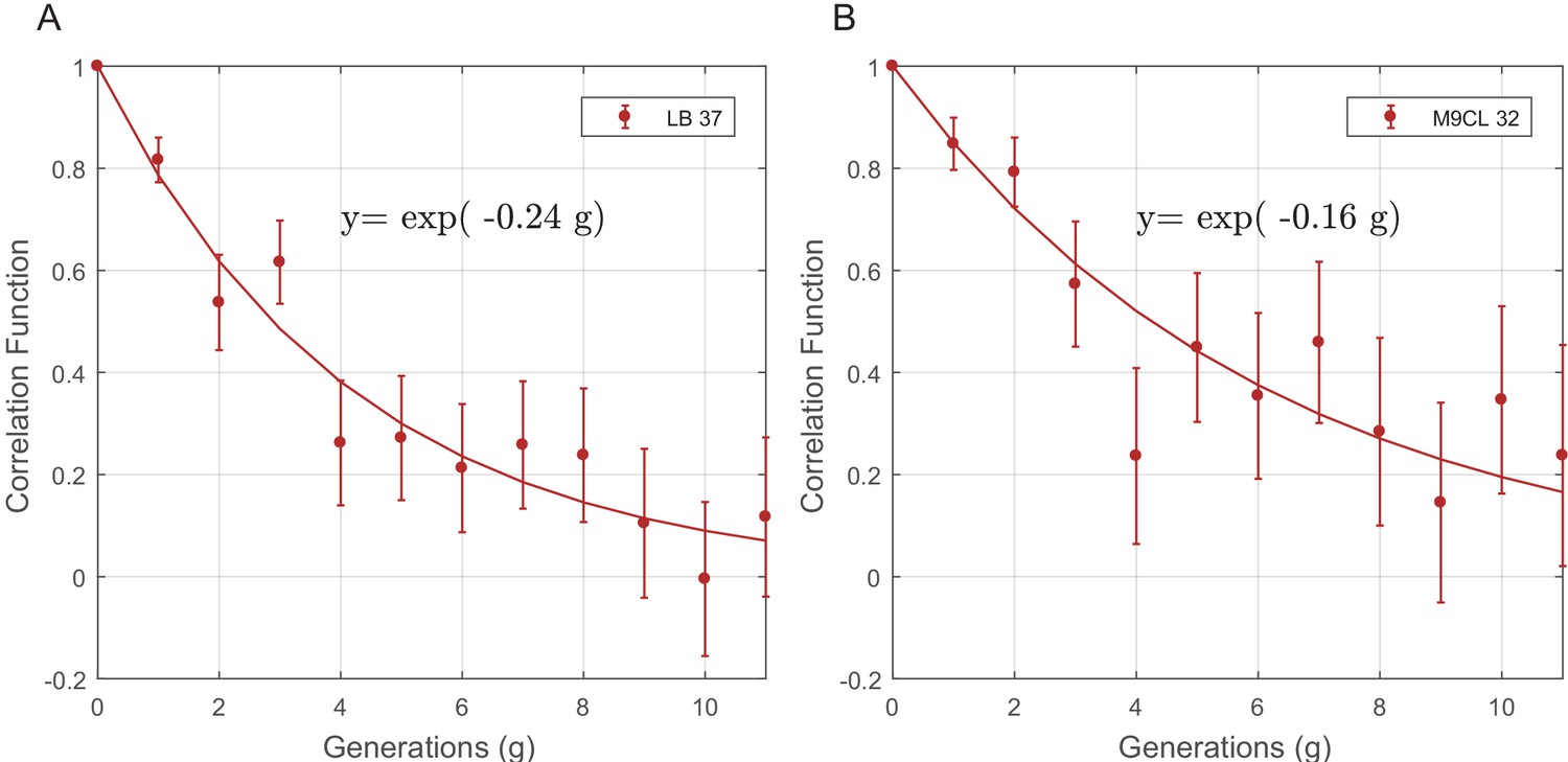
The PCF of cell-cycle time (T) for SCs in different growth conditions.
The PCF of SCs cell-cycle time in LB at 37°C (57 pairs from two separate experiments) (A) and in M9CL at 32°C (29 pairs from two separate experiments) (B). Existence of strong correlation between cell-cycle duration in both (A) and (B) demonstrates the robustness of non-genetic restraint in different experimental conditions. The lines in both graphs are the best fits to the data depicted in the graphs. The decay rate of the correlation in both cases is very similar to that observed in LB medium at 32°C described in the main text (y=exp(−0.23 g)).
Figure 4—figure supplement 4
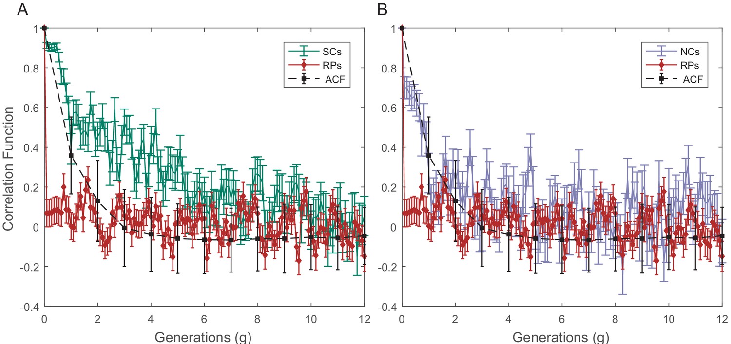
Raw PCF values of cell size as a function of time for SCs, NCs, and RPs.
The cell size PCF for SCs (A) and for NCs (B) are compared in both graphs with the cell size ACF and PCF for RPs. Sister cells show strong cell size correlation that decays slowly over a long time. NCs show almost no correlation in cell size similar to ACF of initial sizes. For details of the PCF and errors calculations, refer to earlier SI.
Figure 4—figure supplement 5
PCF values of cell size and cell-cycle duration as a function of time for NCs with different starting sizes.
PCF of cell-cycle time (A) and cell length (B) for NCs starting from random initial sizes are compared in both graphs with ACF and PCF for RPs. NCs starting with random initial sizes show almost no correlation in cell size or cell-cycle time similar to RPs.
Figure 5 with 4 supplements
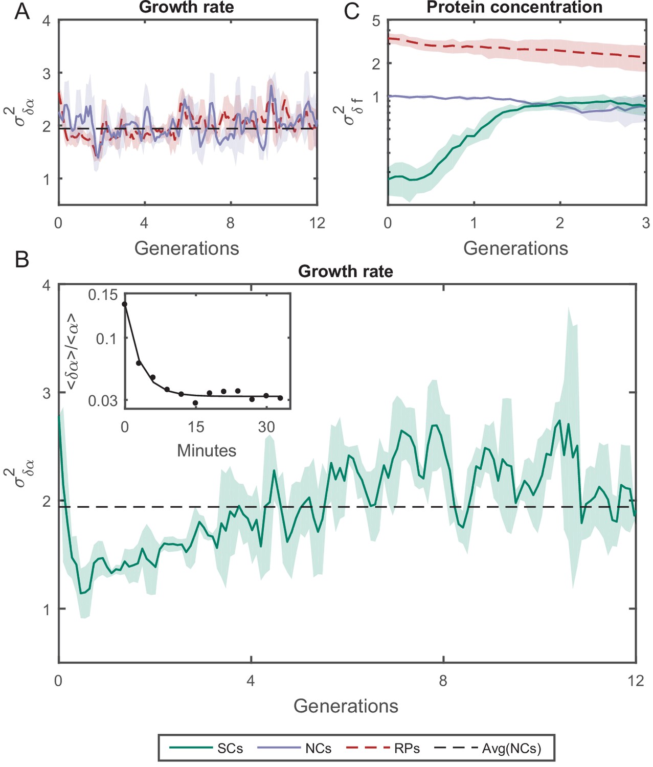
Variance () as a function of the time.
(A) of the growth rate difference () between cell pairs for NCs and RPs as a function of time (see Figure 5—figure supplement 3 for the details of the calculation). The variance for both pair types does not change over time. (B) of SCs, on the other hand, exhibits large variance immediately after separation (∼50%) higher than NCs and RPs and rapidly drops to its minimum value within one generation time (∼30 min), and increases thereafter for 4 hr (∼8 generations) until saturating at a fixed value equivalent to that observed for NCs and RPs. Each point in A and B is the average over three frames moving window, and the shaded area represents the standard deviation of that average. (C) Unlike , δf of SCs increases to its saturation value within ∼2 generations (see Figure 5—figure supplement 4 for the details of the calculation). Here, each point represents the average of three different experiments, and the shaded part represents the standard deviation.
Figure 5—figure supplement 1
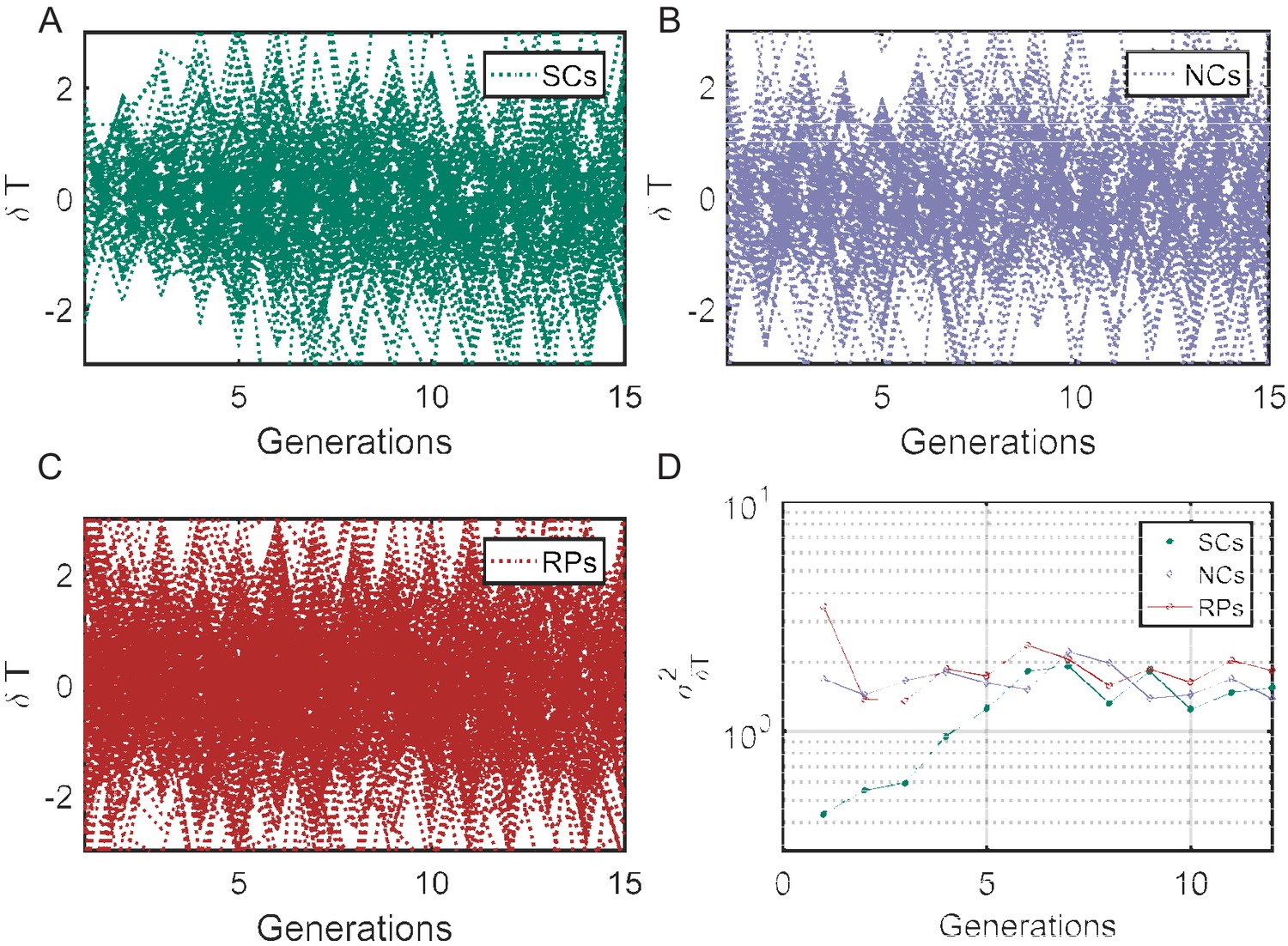
Cell-cycle time variance () as a function of time.
(A–C) Individual traces showing difference in cell-cycle times () for SCs, NCs, and RPs, respectively. The variance () of cell cycles times differences () as a function of time (D) represent the variance of the plots in (A–C) calculated at different time points using . for SCs starts from a small value in first generation and saturate to a constant value after ∼7 generations (similar to the time scale obtained from the PCF ∼8 generations), while for NCs and RPs remain constant over time.
Figure 5—figure supplement 2
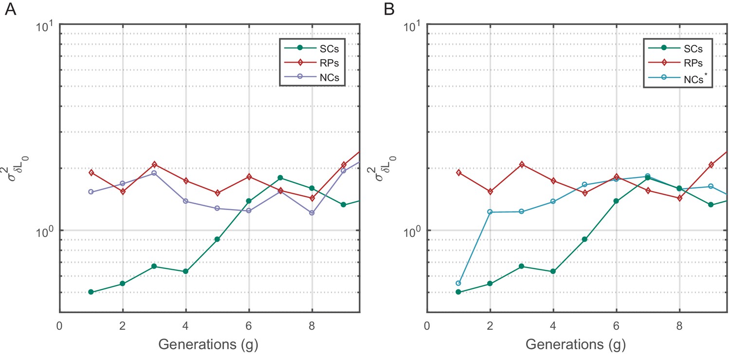
Cell size variance () as a function of time.
Birth size variance was calculated similar to in Figure 5—figure supplement 1. for SCs increases slowly and saturates at a fixed value after ∼7 generations (mean lifetime ∼3.5 generations) similar to the time scale observed in the PCF. For NCs with random initial sizes (A), remains constant similar to RPs. for NCs with similar birth sizes starts from a value similar to SCs but shoots up to the saturation value within one generation.
Figure 5—figure supplement 3
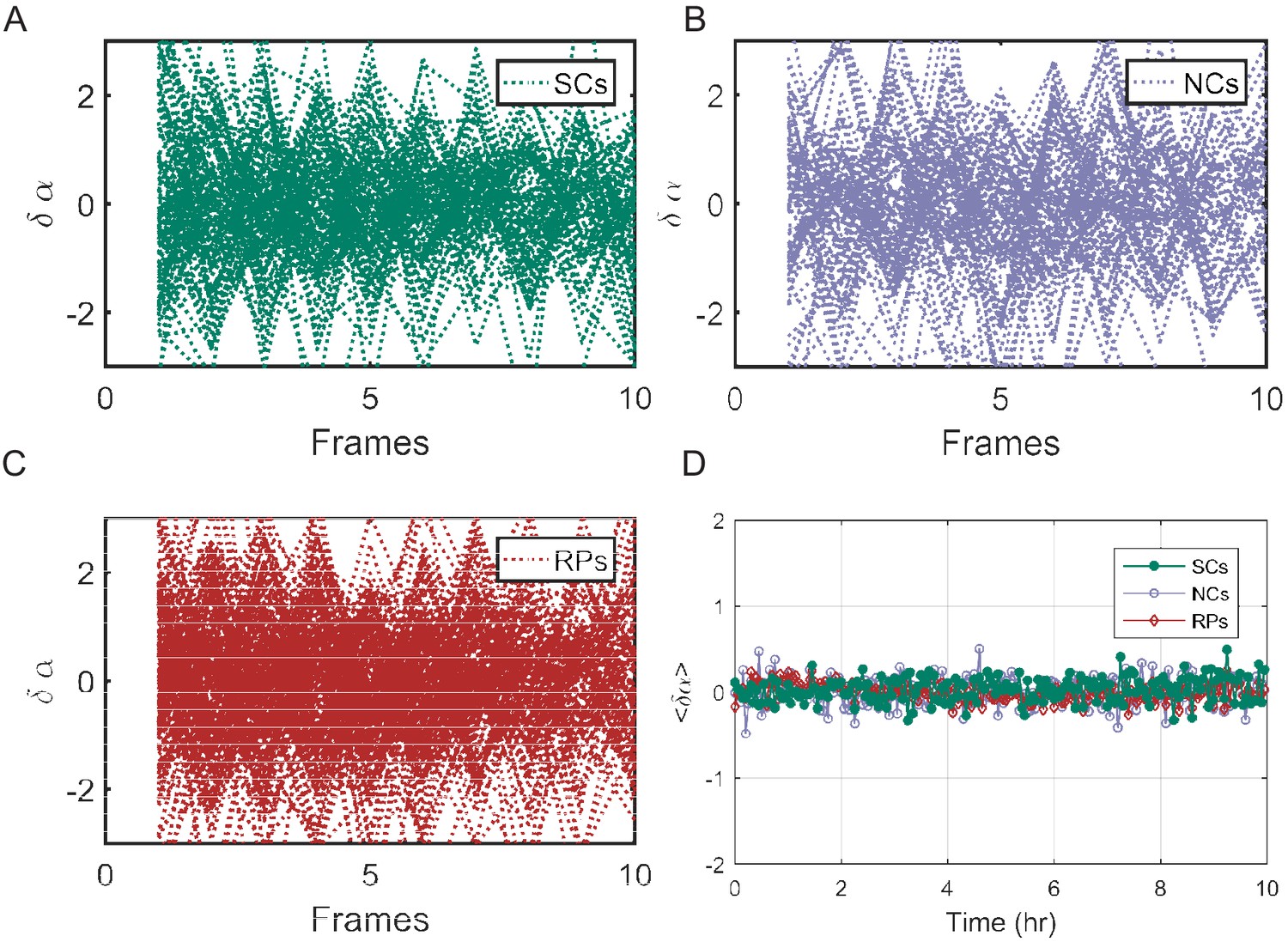
Exponential elongation rate difference () as a function of time.
Individual traces showing the difference between the exponential elongation rates () for SCs (A), NCs (B), and RPs (C). (D) The mean of for all cell pairs remains zero along time as expected. For details of calculations, please refer to the main text.
Figure 5—figure supplement 4
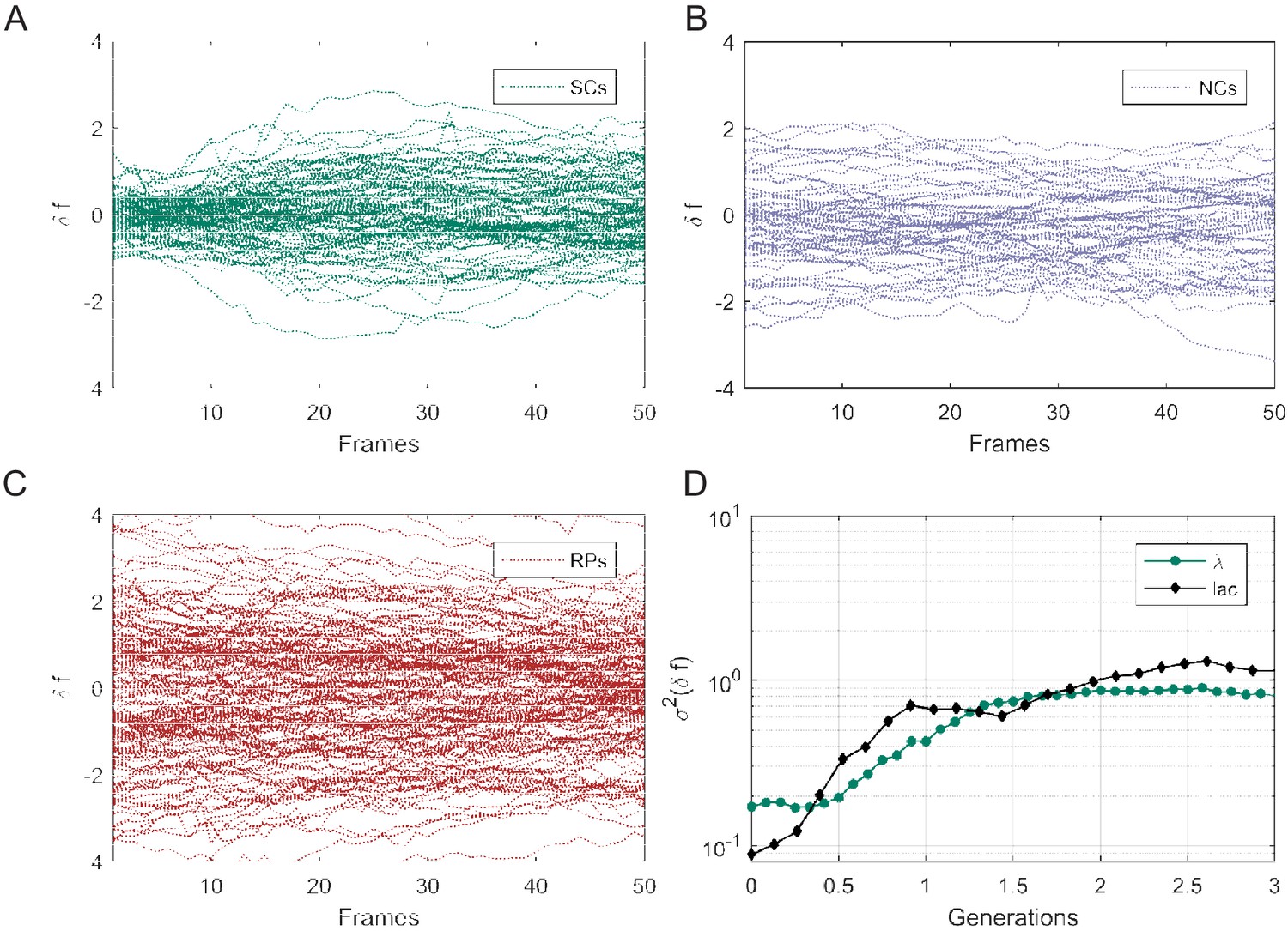
Mean fluorescence variance () as a function of time.
Individual traces showing the difference in mean fluorescence intensity (δf) of gfp expressed in SCs (A), NCs (B), and RPs (C). (D) The variance ( calculated similarly to in Figure 5—figure supplement 1) of GFP expressed under the control of the Lac Operon promoter in lactose medium (metabolically relevant) is compared with that of GFP expressed under the control of the Pr promoter in LB medium (metabolically irrelevant). It is clear that both exhibit no significant difference and a very short memory (≤2 generations).
Tables
Key resources table
| Reagent type (species) or resource | Designation | Source or reference | Identifiers | Additional information |
|---|---|---|---|---|
| Strain, strain background (Escherichia coli) | MG1655 | Coli Genetic Stock Center (CGSC) | 6300 | F-, , rph-1 |
| Recombinant DNA reagent | pZA3R-GFP | Lutz and Bujard, 1997 | https://academic.oup.com/nar/article/25/6/1203/1197243 | GFP expressed from the λ Pr promoter |
| Recombinant DNA reagent | pZA32wt-GFP | Lutz and Bujard, 1997 | https://academic.oup.com/nar/article/25/6/1203/1197243 | GFP expressed from the LacO promoter |
| Software, algorithm | MATLAB | MathWorks | N/A | |
| Software, algorithm | Oufti | Paintdakhi et al., 2016 | http://oufti.org/ |
Appendix 1—table 1
The calculated values of the PCF for SCs were verified by calculating the slopes of best fits to the plots of TimeA vs TimeB graphs (Figure 4—figure supplement 2).
| Generation | PCF | Slope of best fit line (Figure 4—figure supplement 2) |
|---|---|---|
| 1st | 0.86 ± 0.02 | 0.87 |
| 2nd | 0.65 ± 0.05 | 0.69 |
| 3rd | 0.54 ± 0.06 | 0.44 |
| 4th | 0.36 ± 0.07 | 0.42 |
| 5th | 0.28 ± 0.08 | 0.25 |
| 6th | 0.23 ± 0.08 | 0.25 |
| 7th | 0.12 ± 0.09 | 0.11 |
| 8th | 0.23 ± 0.09 | 0.25 |
| 9th | 0.00 ± 0.09 | 0.00 |
Additional files
Download links
A two-part list of links to download the article, or parts of the article, in various formats.
Downloads (link to download the article as PDF)
Open citations (links to open the citations from this article in various online reference manager services)
Cite this article (links to download the citations from this article in formats compatible with various reference manager tools)
Non-genetic inheritance restraint of cell-to-cell variation
eLife 10:e64779.
https://doi.org/10.7554/eLife.64779


