Decoding subjective emotional arousal from EEG during an immersive virtual reality experience
- Department of Neurology, Max Planck Institute for Human Cognitive and Brain Sciences, Germany
- Humboldt-Universität zu Berlin, Faculty of Philosophy, Berlin School of Mind and Brain, Germany
- Sackler Centre for Consciousness Science, School of Engineering and Informatics, University of Sussex, United Kingdom
- Sussex Neuroscience, School of Life Sciences, University of Sussex, United Kingdom
- Bernstein Center for Computational Neuroscience Berlin, Germany
Figures
Figure 1
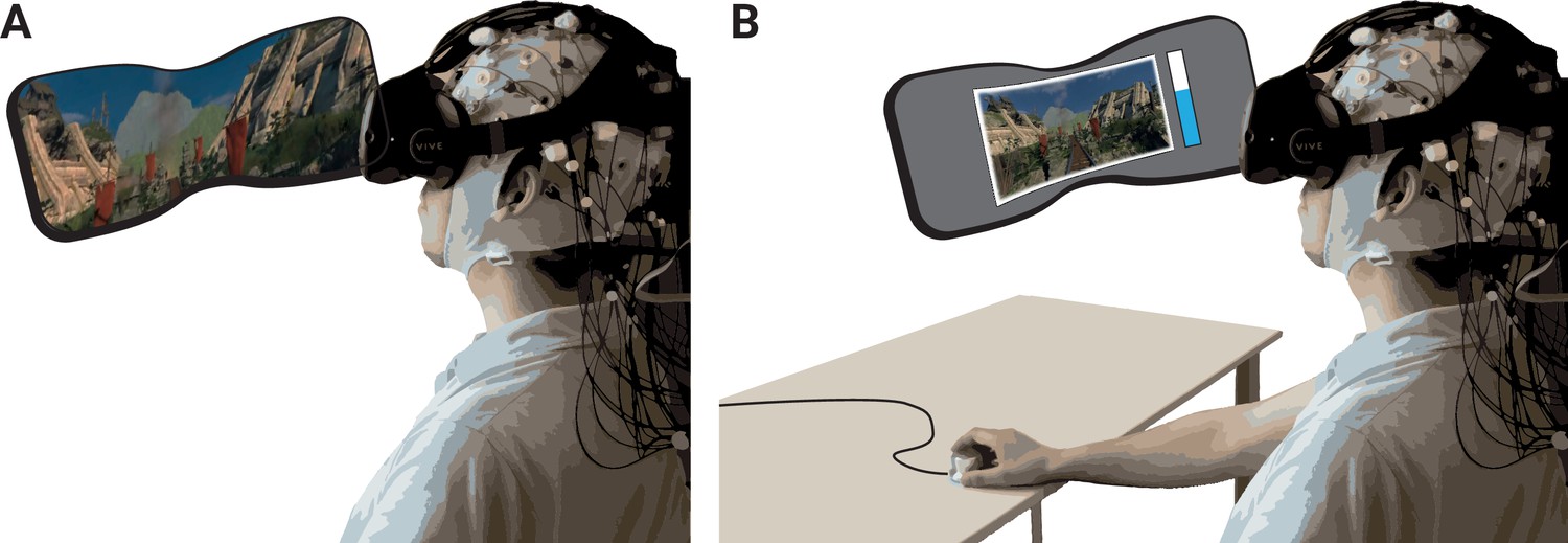
Schematic of experimental setup.
(A) The participants underwent the experience (two rollercoasters separated by a break) in immersive virtual reality (VR), while EEG was recorded. (B) They then continuously rated the level of emotional arousal with a dial viewing a replay of their experience. The procedure was completed twice, without and with head movements.
Figure 2

Group averaged power spectra for the two emotional arousal levels (low, high) and head movement conditions (nomov, mov).
Thick lines represent the mean log-transformed power spectral density of all participants and electrodes. Shaded areas indicate the standard deviation of the participants. High and low emotional arousal are moments that have been rated as most (top tertile) and least arousing (bottom tertile), respectively (the middle tertile was discarded; see main text). The power spectra were produced using MATLAB’s pwelch function with the same data (after ICA correction and before spatio-spectral decomposition [SSD] filtering) and parameters as the individual alpha peak detection (see Materials and methods section for details). A tabular overview of the alpha peak frequencies of the individual participants is available as Figure 2—source data 1.
-
Figure 2—source data 1
Selected alpha peaks (8–13 Hz) per participant and condition.
Results of FOOF computations for three different conditions: eyes-closed resting state, nomov, and mov.
- https://cdn.elifesciences.org/articles/64812/elife-64812-fig2-data1-v2.csv
Figure 3

Schematic of the selection of individual alpha components using spatio-spectral decomposition (SSD).
(Left) 1/f estimation (dotted grey line) to detrend SSD components (solid turquoise line). (Right) After detrending the signal, components were selected, whose peak in the detrended alpha window (centred at the individual alpha peak, vertical dotted grey line) was (A) > 0.35 V2/Hz (indicated by horizontal dotted red line) and (B) higher than the bigger of the two mean amplitudes of the adjacent frequency flanks (2 Hz width).
Figure 4
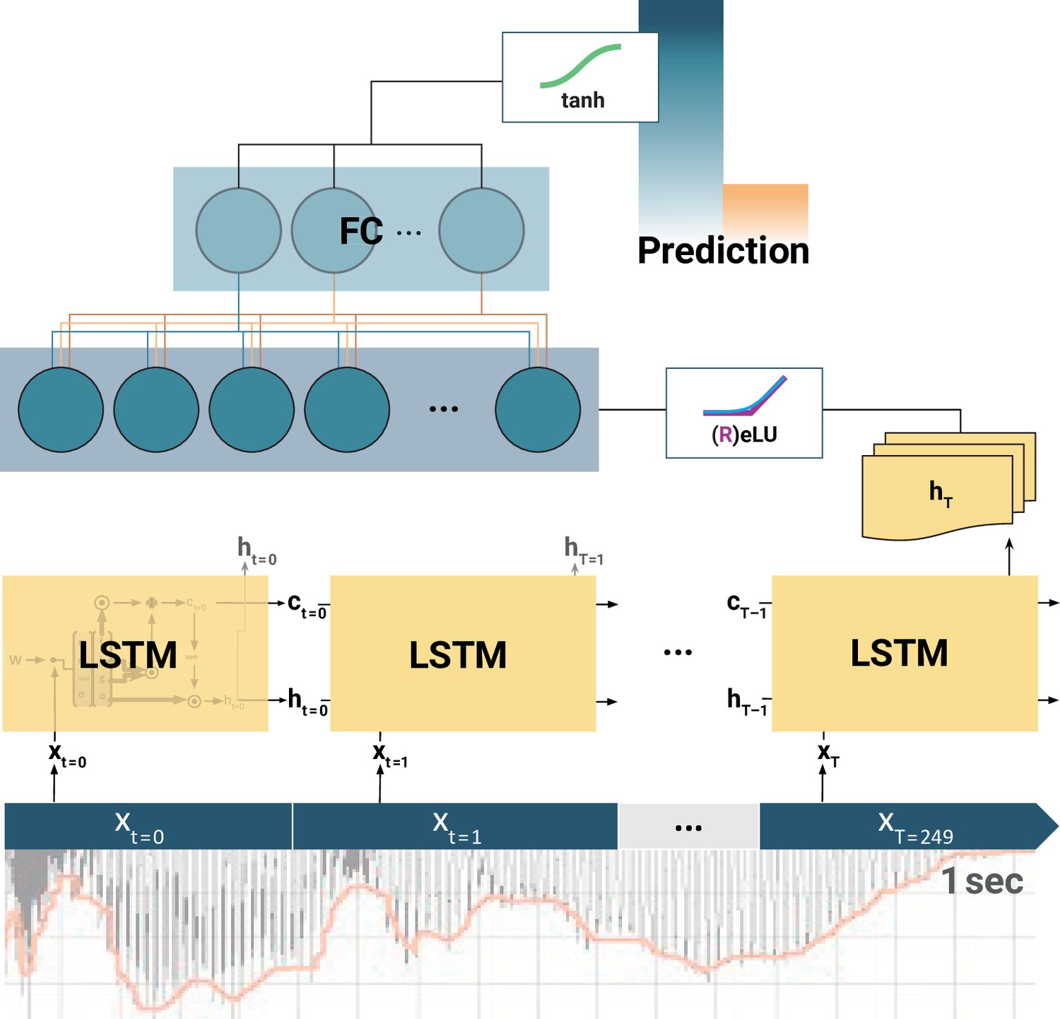
Schematic of the long short-term memory (LSTM) recurrent neural network (RNN).
At each training step, the LSTM cells successively slide over 250 data arrays of neural components (xt=0, xt=1,..., xT=249) corresponding to 1 s of the EEG recording. At each step t, the LSTM cell computes its hidden state ht. Only the final LSTM output (hT) at time-step T = 249 is then fed into the following fully connected (FC) layer. The outputs of all (LSTMs, FCs) but the final layer are normalized by rectified linear units (ReLU) or exponential linear units (ELU). Finally, the model prediction is extracted from the last FC layer via a tangens hyperbolicus (tanh). Note: depending on model architecture, there were one to two LSTM layers, and one to two FC layers. The hyperparameter constellations that yielded the highest accuracy for the individual participants per movement condition are available as Figure 4—source data 1.
-
Figure 4—source data 1
Long short-term memory (LSTM) hyperparameter search per movement condition.
LSTM: number of cells per layer. FC: number of hidden units in fully connected layer, before final output neuron. l.rate: learning rate. reg.: type of weight regularizer. reg. strength: respective regularization strength. activ.func: intermediate layer activation function. components: individually selected components for training after spatio-spectral decomposition (SSD) selection.
- https://cdn.elifesciences.org/articles/64812/elife-64812-fig4-data1-v2.zip
Figure 5 with 1 supplement
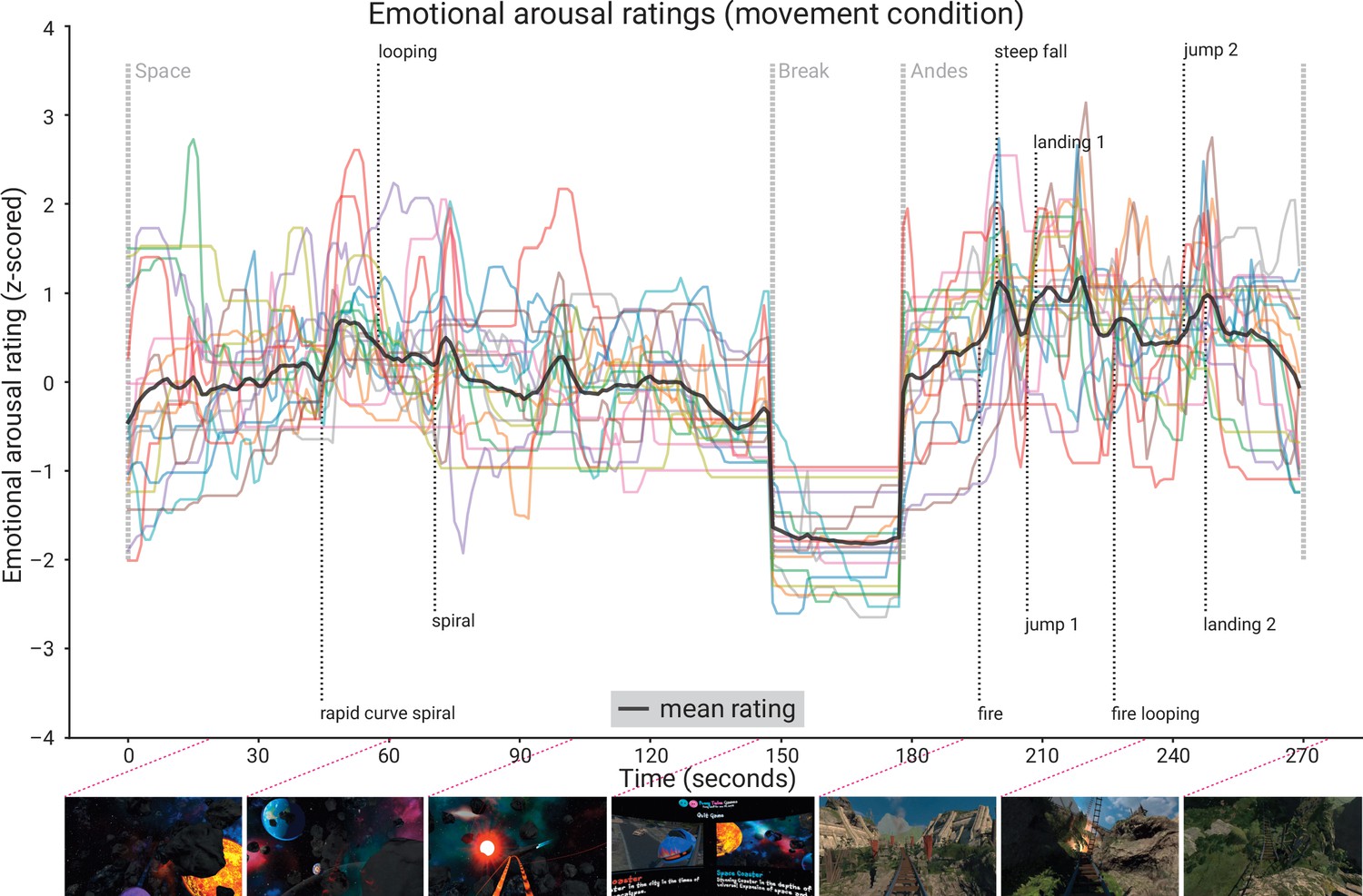
Subjective emotional arousal ratings (movement condition).
Emotional arousal ratings of the experience (with head movement; see Figure 5—figure supplement 1 for the ratings from the no-movement condition). Coloured lines: individual participants; black line: mean across participants; vertical lines (light grey): beginning of the three phases (Space Coaster, Break, Andes Coaster); vertical lines (dark grey): manually labelled salient events (for illustration). Bottom row: exemplary screenshots of the virtual reality (VR) experience. The ratings for the condition without head movement are shown in the figure supplement.
Figure 5—figure supplement 1

Subjective emotional arousal ratings (no-movement condition).
Emotional arousal ratings of the experience (without head movement). Coloured lines: individual participants; black line: mean across participants; vertical lines (light grey); beginning of the three phases (Space Coaster, Break, Andes Coaster); vertical lines (dark grey): manually labelled salient events (for illustration).
Figure 6 with 1 supplement

Spatial patterns resulting from spatio-spectral decomposition (SSD), source power comodulation (SPoC), and common spatial pattern (CSP) decomposition.
Colours represent absolute normalized pattern weights (inverse filter matrices) averaged across all subjects per condition (nomov: without head movement, mov: with head movement). Before averaging, the pattern weight vectors of each individual subject were normalized by their respective L2-norm. To avoid cancellation due to the non-polarity-aligned nature of the dipolar sources across subjects, the average was calculated from the absolute pattern weights. SSD allows the extraction of components with a clearly defined spectral peak in the alpha frequency band. Shown are the patterns associated with the four SSD components that yielded the best signal-to-noise ratio (left column). The SSD filtered signal was the input for the decoding approaches SPoC, CSP, and LSTM: SPoC adds a spatial filter, optimizing the covariance between the continuous emotional arousal ratings and alpha power. Shown here is the pattern of the component which – in line with our hypothesis – maximized the inverse relationship between emotional arousal and alpha power. CSP decomposition yielded components with maximal alpha power for low-arousing epochs and minimal for high-arousing epochs (bottom row in the CSP panel) or vice versa (upper row in the CSP panel). The high correspondence between the patterns resulting from SPoC and CSP seems to reflect that both algorithms converge to similar solutions, capturing alpha power modulations in parieto-occipital regions as a function of emotional arousal. The spatial patterns for the individual subjects are displayed in the figure supplement. (Note: as the LSTM results cannot be topographically interpreted, they are not depicted here.)
Figure 6—figure supplement 1
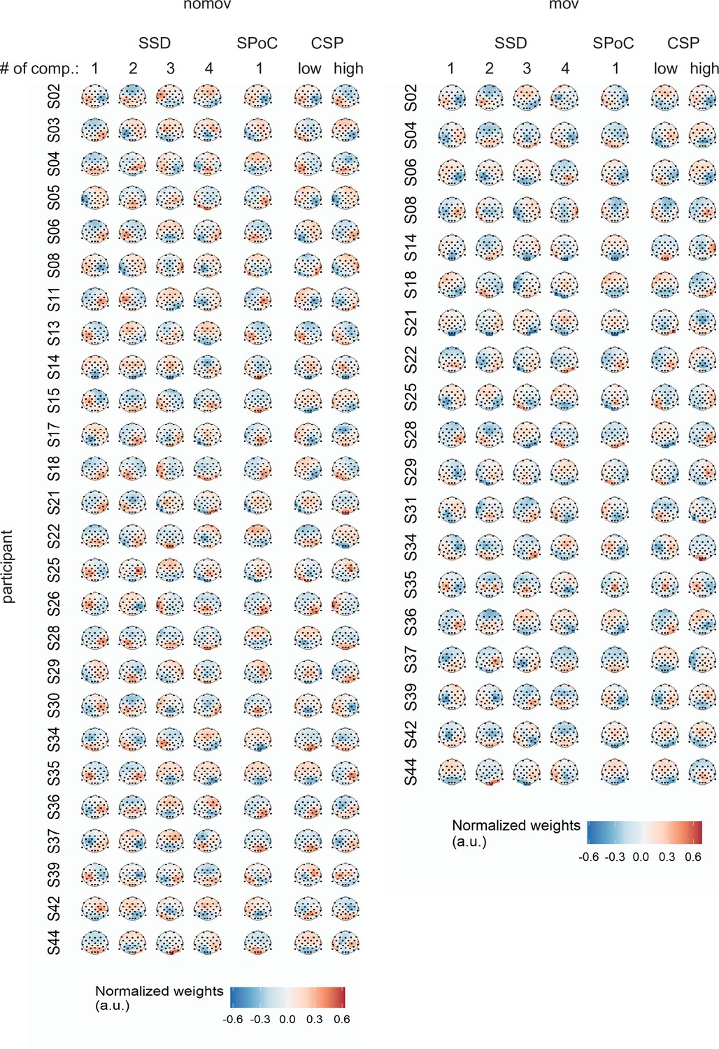
Spatial patterns per single subject and movement condition yielded by the different spatial signal decompositions.
For spatio-spectral decomposition (SSD) the four patterns corresponding to the four highest eigenvalues among the accepted components (see Materials and methods) are displayed (note: subjects with less than four accepted SSD components were discarded for further analysis; for subjects with more than four accepted components, all of these components went into the further analyses but only the first four patterns are shown here). For source power comodulation (SPoC) the pattern associated with the component that yielded the strongest correlation between target and source power is displayed. For common spatial patterns (CSP) the patterns associated with the components that maximized power during states of low and high emotional arousal are shown.
Figure 7
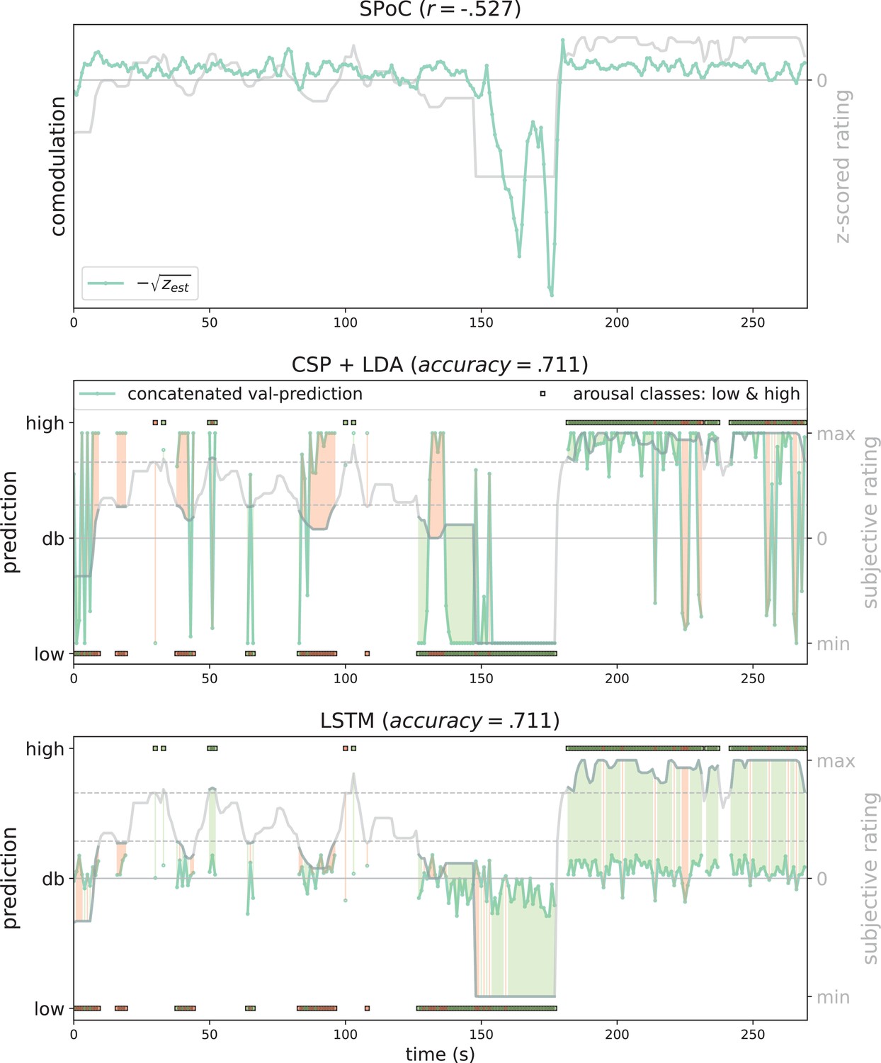
Exemplary model predictions.
Predictions (turquoise line, dots) across models trained on the data of one participant in the movement condition (source power comodulation [SPoC]: normalized negative zest, here comodulation; common spatial patterns [CSP]: posterior probability; long short-term memory [LSTM]: tanh output). Top row: most negatively correlating SPoC component (for visualization we depict the normalized and mean-centred value of the rating and of the negative square root of zest). Middle and lower row: model predictions on validation sets (across the cross-validation splits) for CSP and LSTM, respectively. The grey curvy line in each panel indicates the continuous subjective rating of the participant. Horizontal dotted lines indicate the class borders. The area between these lines is the mid-tertile which was discarded for CSP and LSTM analyses. Class membership of each rating sample (1 s) is indicated by the circles at the top and bottom of the rating. A model output falling under or above the decision boundary (db) indicates the model prediction for one over the other class, respectively. The correct or incorrect prediction is indicated by the colour of the circle (green and red, respectively), and additionally colour-coded as area between model output (turquoise) and rating.
Figure 8

Comparison of the binary decoding approaches.
Confusion matrices of the classification accuracies for higher and lower self-reported emotional arousal using long short-term memory (LSTM) (lower row) and common spatial patterns (CSP) (upper row) in the condition without (left column) and with (right column) head movement. The data underlying this figure can be downloaded as Figure 8—source data 1.
-
Figure 8—source data 1
Prediction tables of the binary decoding models.
The zip file contains a folder for each of the movement conditions (with and without head movements) with subfolders for the binary decoding approaches (common spatial patterns [CSP], long short-term memory [LSTM]). Each folder includes three types of tables with the same format (Subjects × Samples). Subjects (N varies by condition) who went into the final classification (after removals during preprocessing). Samples (N = 270) refer to the sequential seconds of the experience (total length: 270 s). Each cell contains: targetTable: the target/ground truth assigned to this sample (by binning the continuous rating). CSP: 1=Low Arousal, 2=High Arousal, NaN = Medium Arousal; LSTM: –1=Low Arousal, 1=High Arousal, 0=Medium Arousalprediction. TableProbabilities: the probability/certainty of this sample to be classified as ‘High Arousing’ (positive probabilities) or ‘Low Arousing’ (negative probabilities). predictionTable: the binarized version of the probabilities. CSP: 1=High Arousal, 0=Low Arousal, NaN = Medium Arousal, LSTM: 1=High Arousal, –1=Low Arousal, 0=Medium Arousal.
- https://cdn.elifesciences.org/articles/64812/elife-64812-fig8-data1-v2.zip
Figure 9
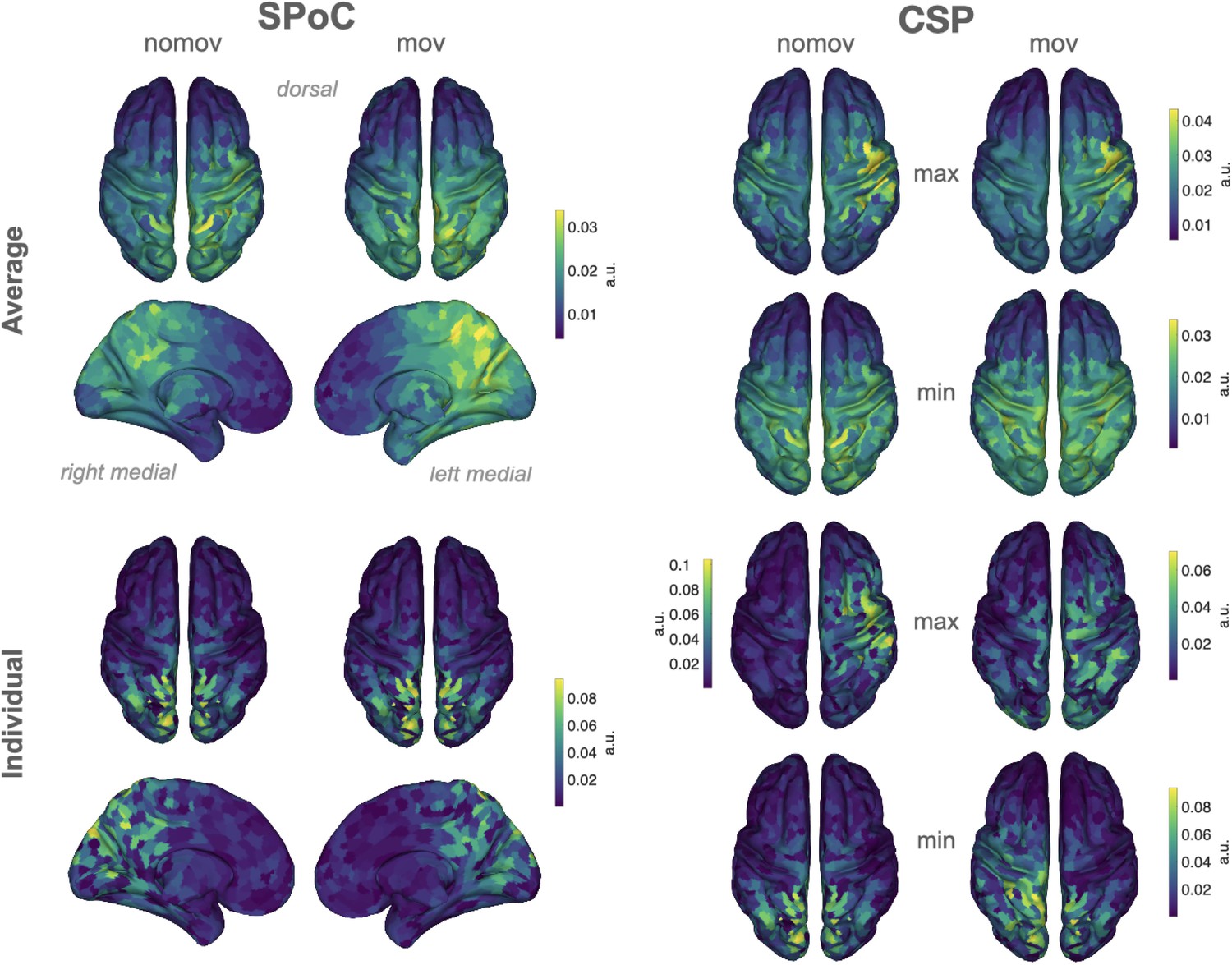
Source reconstructions (exact low resolution tomography analysis [eLORETA]).
The projection of source power comodulation (SPoC) and common spatial patterns (CSP) components in source space confirms the link between emotional arousal and alpha oscillations in parieto-occipital regions. Colours represent the inversely modelled contribution of the cortical voxels to the respective spatial pattern yielded by SPoC or CSP (max: component maximizing power for epochs of high arousal; min: component minimizing power for epochs of high arousal). We applied the same normalization and averaging procedures as for the topoplots in Figure 6. Upper row: averaged across all subjects per condition (nomov, mov). Lower row: patterns of one individual (the same as in Figure 7).
Figure 10

Correlation of performances across methods (source power comodulation [SPoC], common spatial pattern [CSP], long short-term memory [LSTM]) and conditions (nomov: without head movement, mov: with head movement).
The model performance metrics are classification accuracy (CSP and LSTM) and correlation coefficients (SPoC; note: based on our hypothesis of an inverse relationship between emotional arousal and alpha power, more negative values indicate better predictive performance). Plots above and below the diagonal show data from the nomov (yellow axis shading, upper right) and the mov (blue axis shading, lower left) condition, respectively. Plots on the diagonal compare the two conditions (nomov, mov) for each method. In the top left corner of each panel, the result of a (Pearson) correlation test is shown. Lines depict a linear fit with the 95% confidence interval plotted in grey. The data underlying this figure can be downloaded as Figure 10—source data 1.
-
Figure 10—source data 1
Decoding results per decoding approach, movement condition, and participant.
The data file contains a data frame per movement condition (nomov, mov) with following columns (for source power comodulation [SPoC] all values relate to the component with the smallest [i.e., most negative] correlation between its alpha power and the emotional arousal ratings). Subject; SPOC_LAMBDA: covariance; SPOC_CORR: Pearson correlation coefficient; SPOC_Pvalue: p-values obtained from the permutation test (see Materials and methods) on the single subject level; CSP_acc and LSTM_acc: proportion of correctly classified samples across the cross-validation folds. CSP_Pvalues and LSTM_Pvalues: p-values obtained from the exact binomial test on the single-subject level (see Materials and methods).
- https://cdn.elifesciences.org/articles/64812/elife-64812-fig10-data1-v2.zip
Author response image 1
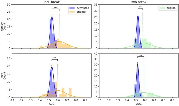
CSP decoding performance shown as distributions of the means of the permuted null distributions (blue) over all subjects next to the distribution of the original, unpermuted decoding scores (yellow/green) on data with (left column) and without the break (right column) as well as with (lower row, “mov”) and without (upper row, “nomov”) free head movement.
One-sided paired t-tests indicate that the means of these distributions (dotted vertical lines) differ significantly, with higher performance when decoding from the unpermuted arousal ratings for all conditions (ns: not significant, *: p <.05, **: p <.01, ***: p <.001).
Author response image 2

Logistic regression decoding performance across subjects was significantly above chance level (permuted arousal ratings with 1000 permutations) in all but the condition without head movement and without the break.
(For more details, please refer to the caption of Author response image 1).
Author response image 3
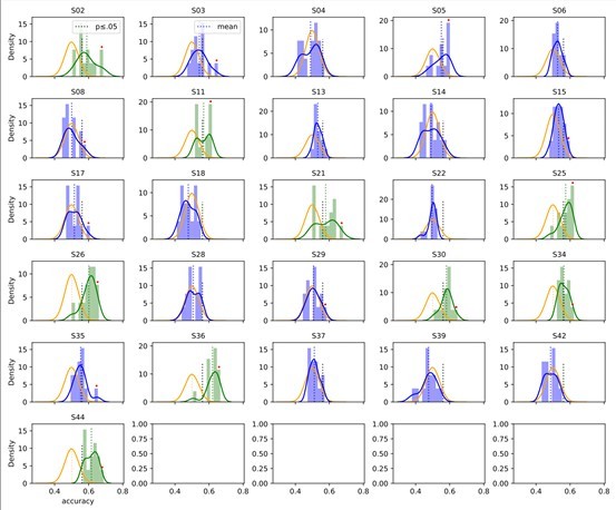
Accuracy over the narrow set of hyperparameter (HP) settings in the condition without free head movement (nomov).
The average accuracy of HPsets was (green) or was not (blue) significant. Orange: Binomial distribution over random trials. Black thick dotted line: Significance threshold. Red dots indicate the originally significant subjects and their best performing HP set. If the mean of the HP-set distribution (longer, dotted vertical line) passes the p-value threshold (shorter, black-dotted vertical line), the average accuracy is significant (distribution becomes green, otherwise blue).
Author response image 4

Accuracy over the narrow set of hyperparameter (HP) settings in mov conditions.
For details, please see the caption of Author response image 3A.
Tables
Author response table 1
Number of participants, for which the level of emotional arousal (low, high) could be significantly predicted from α power (on data including break).
| Significant prediction | nomov | mov |
|---|---|---|
| Logistic regression | 5/26 | 4/19 |
| CSP | 9/26 | 5/19 |
Additional files
Download links
A two-part list of links to download the article, or parts of the article, in various formats.
Downloads (link to download the article as PDF)
Open citations (links to open the citations from this article in various online reference manager services)
Cite this article (links to download the citations from this article in formats compatible with various reference manager tools)
Decoding subjective emotional arousal from EEG during an immersive virtual reality experience
eLife 10:e64812.
https://doi.org/10.7554/eLife.64812


