Research Article

Neuroscience

Decoding subjective emotional arousal from EEG during an immersive virtual reality experience

Department of Neurology, Max Planck Institute for Human Cognitive and Brain Sciences, Germany
Humboldt-Universität zu Berlin, Faculty of Philosophy, Berlin School of Mind and Brain, Germany
Sackler Centre for Consciousness Science, School of Engineering and Informatics, University of Sussex, United Kingdom
Sussex Neuroscience, School of Life Sciences, University of Sussex, United Kingdom
Bernstein Center for Computational Neuroscience Berlin, Germany

Oct 28, 2021

https://doi.org/10.7554/eLife.64812

Version of Record

Accepted for publication after peer review and revision.

Download
Cite
Share
CommentOpen annotations (there are currently 0 annotations on this page).

Version of Record published: December 15, 2021 (This version)
Accepted Manuscript published: October 28, 2021 (Go to version)
Accepted: October 27, 2021
Received: November 11, 2020
Preprint posted: October 25, 2020 (Go to version)

1. Of interest
APOE expression and secretion are modulated by mitochondrial dysfunction

Meghan E Wynne, Oluwaseun Ogunbona ... Victor Faundez

Research Article Updated May 31, 2023
Further reading

Article
Figures and data
Abstract
Editor's evaluation
eLife digest
Introduction
Materials and methods
Results
Discussion
Appendix 1
Data availability
References
Decision letter
Author response
Article and author information
Metrics

Abstract

Immersive virtual reality (VR) enables naturalistic neuroscientific studies while maintaining experimental control, but dynamic and interactive stimuli pose methodological challenges. We here probed the link between emotional arousal, a fundamental property of affective experience, and parieto-occipital alpha power under naturalistic stimulation: 37 young healthy adults completed an immersive VR experience, which included rollercoaster rides, while their EEG was recorded. They then continuously rated their subjective emotional arousal while viewing a replay of their experience. The association between emotional arousal and parieto-occipital alpha power was tested and confirmed by (1) decomposing the continuous EEG signal while maximizing the comodulation between alpha power and arousal ratings and by (2) decoding periods of high and low arousal with discriminative common spatial patterns and a long short-term memory recurrent neural network. We successfully combine EEG and a naturalistic immersive VR experience to extend previous findings on the neurophysiology of emotional arousal towards real-world neuroscience.

Editor's evaluation

Hofmann et al., investigate the link between two phenomena, emotional arousal and cortical α activity. Although α activity is tightly linked to the first reports of electric activity in the brain nearly 100 years ago, a comprehensive characterization of this phenomenon is elusive. One of the reasons is that EEG, the major method to investigate electric activity in the human brain, is susceptible to motion artifacts and, thus, mostly used in laboratory settings. Here, the authors combine EEG with virtual reality (VR) to give experimental participants a roller coaster ride with high immersion. The ride, literally, leads to large ups and downs in emotional arousal, which is quantified by the subjects during a later rerun. Several different decoding methods were evaluated, and each showed above-chance levels of performance, substantiating a link between lower levels of parietal/occipital α and subjective arousal in a quasi-naturalistic setting.

https://doi.org/10.7554/eLife.64812.sa0

eLife digest

Human emotions are complex and difficult to study. It is particularly difficult to study emotional arousal, this is, how engaging, motivating, or intense an emotional experience is. To learn how the human brain processes emotions, researchers usually show emotional images to participants in the laboratory while recording their brain activity. But viewing sequences of photos is not quite like experiencing the dynamic and interactive emotions people face in everyday life.

New technologies, such as immersive virtual reality, allow individuals to experience dynamic and interactive situations, giving scientists the opportunity to study human emotions in more realistic settings. These tools could lead to new insights regarding emotions and emotional arousal.

Hofmann, Klotzsche, Mariola et al. show that virtual reality can be a useful tool for studying emotions and emotional arousal. In the experiment, 37 healthy young adults put on virtual reality glasses and ‘experienced’ two virtual rollercoaster rides. During the virtual rides, Hofmann, Klotzsche, Mariola et al. measured the participants' brain activity using a technique called electroencephalography (EEG). Then, the participants rewatched their rides and rated how emotionally arousing each moment was. Three different computer modeling techniques were then used to predict the participant’s emotional arousal based on their brain activity.

The experiments confirmed the results of traditional laboratory experiments and showed that the brain’s alpha waves can be used to predict emotional arousal. This suggests that immersive virtual reality is a useful tool for studying human emotions in circumstances that are more like everyday life. This may make future discoveries about human emotions more useful for real-life applications such as mental health care.

Introduction

While humans almost constantly interact with complex, dynamic environments, lab-based studies typically use simplified stimuli in passive experimental situations. Trading realism for experimental control happens at the expense of the representativity of the experimental design (Brunswik, 1955), that is, the degree to which effects found in the lab generalize to practical everyday-life conditions. This may be particularly true for affective phenomena like emotions.

Emotional arousal as a fundamental property of affective experience

Emotions are subjective, physiological, and behavioural responses to personally meaningful external stimuli (Mauss and Robinson, 2009) or self-generated mental states (e.g., memories; Damasio et al., 2000) and underlie our experience of the world (James, 1884; James, 1890; Seth, 2013). Emotions are crucial for physical and mental health (Gross and Muñoz, 1995) and their investigation has long been at the core of experimental psychology (Wundt and Judd, 1897).

Dimensional accounts conceptualize emotions along the two axes of valence and arousal (Duffy, 1957; Kuppens et al., 2013; Russell, 1980; Russell and Barrett, 1999; Wundt and Judd, 1897): valence differentiates states of pleasure and displeasure, while emotional arousal describes the degree of activation or intensity that accompanies an emotional state. [Different types of arousal have been proposed and investigated, such as sexual, autonomic, emotional (Russell, 1980); also in the context of altered states of consciousness, for example, through anaesthesia or sleep. They may share psychological (e.g., increase in sensorimotor and emotional reactivity; Pfaff et al., 2012) and physiological aspects (e.g., sympathetic activation) but are not synonymous. We here explicitly refer to arousal in the context of the subjective experience of emotions].

Emotions have been linked to activity in the autonomic (ANS) and the central nervous system (Dalgleish, 2004). It has thereby been difficult to consistently associate individual, discrete emotion categories with specific response patterns in the ANS (Kragel and Labar, 2013; Kreibig, 2010; Siegel et al., 2018) or in distinct brain regions (Lindquist et al., 2012; but Saarimäki et al., 2016). Rather, emotions seem to be dynamically implemented by sets of brain regions and bodily activations that are involved in basic, also non-emotional psychological operations (i.e., ‘psychological primitives’; Lindquist et al., 2012). In this view, humans are typically in fluctuating states of pleasant or unpleasant arousal (‘core affect’; Russell and Barrett, 1999; Lindquist, 2013), which can be influenced by external stimuli. Emotional arousal could thereby be a ‘common currency’ to compare different stimuli or events (Lindquist, 2013) and represent fundamental neural processes that underlie a variety of emotions (Wilson-Mendenhall et al., 2013). It can fluctuate quickly – on the order of minutes (Kuppens et al., 2010) or seconds (Mikutta et al., 2012) – and has been connected to ANS activity, as measured by pupil diameter (Bradley et al., 2008) or skin conductance (Bach et al., 2010). At the brain level, emotional arousal was linked to lower alpha power, particularly over parietal electrodes (Luft and Bhattacharya, 2015; Koelstra et al., 2012). The parieto-occipital alpha rhythm, typically oscillating in the frequency range of 8–13 Hz, is the dominant EEG rhythm in awake adults with eyes closed (Berger, 1929), where it varies with vigilance (Olbrich et al., 2009). However, in tasks of visual processing (i.e., with eyes open), parieto-occipital alpha power was linked to active attentional processes (e.g., distractor suppression; Kelly et al., 2006; Klimesch, 2012) or, more generally, to functional inhibition for information gating (Jensen and Mazaheri, 2010). Physiologically, alpha oscillations were associated with large-scale synchronization of neuronal activity (Buzsáki, 2006) and metabolic deactivation (Moosmann et al., 2003).

In sum, bodily responses interact in complex ways across situations, and activity in the brain is central for emotions and their subjective component (Barrett, 2017; Seth, 2013). As arousal is a fundamental property not only of emotions but of subjective experience in general (Adolphs et al., 2019), an investigation of its neurophysiology, reflected in neural oscillations, is essential to understanding the biology of the mind.

Studying emotional arousal and its neurophysiology in the lab

Studies that investigated emotions or emotional arousal in laboratory environments typically used static images. For example, more emotionally arousing relative to less emotionally arousing (e.g., neutral) pictures were associated with an event-related desynchronization, that is, a decrease in the power of alpha oscillations in posterior channels (De Cesarei and Codispoti, 2011; Schubring and Schupp, 2019; but Uusberg et al., 2013). In a study, in which emotional arousal was induced through pictures and music, blocks of higher emotional arousal were associated with decreased alpha power compared to blocks of lower emotional arousal (Luft and Bhattacharya, 2015). However, emotion-eliciting content that is repeatedly presented in trials creates an artificial experience for participants (Bridwell et al., 2018); it hardly resembles natural human behaviour and its (neuro-)physiology, which unfolds over multiple continuous timescales (Huk et al., 2018). Moreover, such presentations lack a sense of emotional continuity. External events often do not appear suddenly but are embedded in an enduring sequence, in which emotions build up and dissipate. Real-life scenarios also include anticipatory aspects where emotional components can be amplified or even suppressed, thus rendering the relationship between the corresponding neuronal events and subjective experience more complex than the one typically studied with randomized or partitioned presentations of visual or auditory stimuli.

Virtual reality (VR) technology – particularly immersive VR, in which the user is completely surrounded by the virtual environment – affords the creation and presentation of computer-generated scenarios that are contextually rich and engaging (Diemer et al., 2015). As more naturalistic (i.e., dynamic, interactive, and less decontextualized) experiments allow to study the brain under conditions it was optimized for (Gibson, 1978; Hasson et al., 2020), their findings may more readily generalize to real-world circumstances and provide better models of the brain (Matusz et al., 2019; Shamay-Tsoory and Mendelsohn, 2019).

In this study, we aimed to link subjective emotional arousal with alpha power in a naturalistic setting. Participants completed an immersive VR experience that included virtual rollercoaster rides while their EEG was recorded. They then continuously rated their emotional arousal while viewing a replay of their previous experience (McCall et al., 2015).

Methodological challenges of naturalistic experiments

To tackle the challenges of data acquired in naturalistic settings and with continuous stimuli, we made use of recent advances in signal processing and statistical modelling: spatial filtering methods (originally developed for brain-computer interfaces [BCIs]; Blankertz et al., 2008) have recently gained popularity in cognitive neuroscience (Cohen, 2018; Zuure and Cohen, 2020), where they have been used to analyze continuous data collected in naturalistic experiments, for example, to find inter-subject correlations in neuroimaging data of participants watching the same movie (Dmochowski et al., 2012; Gaebler et al., 2014).

For the present experiment, two spatial filtering methods were applied to link alpha power and subjective emotional arousal: source power comodulation (SPoC; Dähne et al., 2014) and common spatial patterns (CSP; Blankertz et al., 2008; Ramoser et al., 2000).

SPoC is a supervised regression approach, in which a target variable (here: subjective emotional arousal) guides the extraction of relevant M/EEG oscillatory components (here: alpha power). SPoC has been used to predict single-trial reaction times from alpha power in a hand motor task (Meinel et al., 2016), muscular contraction from beta power (Sabbagh et al., 2020), and difficulty levels of a video game from theta and alpha power (Naumann et al., 2016). CSP is used to decompose a multivariate signal into components that maximize the difference in variance between distinct classes (here: periods of high and low emotional arousal). CSP thereby allows optimizing the extraction of power-based features from oscillatory signals, which can then be applied for training classifiers to solve binary or categorical prediction problems. CSP is being used with EEG for BCI (Blankertz et al., 2008) or to decode workload (Schultze-Kraft et al., 2016).

In addition to M/EEG-specific spatial filtering methods, non-linear machine learning methods are suited for the analysis of continuous, multidimensional recordings from naturalistic experiments. Deep neural networks transform high-dimensional data into target output variables (here: different states of emotional arousal) by finding statistical invariances and hidden representations in the input (Goodfellow et al., 2016; LeCun et al., 2015; Schmidhuber, 2015). For time-sequential data, long short-term memory (LSTM) recurrent neural networks (RNNs) are particularly suited (Greff et al., 2017; Hochreiter and Schmidhuber, 1995; Hochreiter and Schmidhuber, 1997). Via nonlinear gating units, the LSTM determines which information flows in and out of the memory cell in order to find long- and short-term dependencies over time. LSTMs have been successfully applied for speech recognition (Graves et al., 2013), language translation (Luong et al., 2015), or scene analysis in videos (Donahue et al., 2015), but also to detect emotions in speech and facial expressions (Wöllmer et al., 2010; Wöllmer et al., 2008) or workload in EEG (Bashivan et al., 2016; Hefron et al., 2017). In comparison to other deep learning methods, LSTMs are ‘quick learners’ due to their efficient gradient flow and thus suitable for the continuous and sparse data recorded under naturalistic stimulation with VR.

The present study tested the hypothesis of a negative association between parieto-occipital alpha power and subjective emotional arousal under dynamic and interactive stimulation. Combining immersive VR and EEG, this study aimed to (1) induce variance in emotional arousal in a naturalistic setting and (2) capture the temporally evolving and subjective nature of emotional arousal via continuous ratings in order to (3) assess their link to oscillations of brain activity in the alpha frequency range. The link between subjective emotional arousal and alpha power was then tested by decoding the former from the latter using the three complementary analysis techniques SPoC, CSP, and LSTM.

Materials and methods

Participants

Forty-five healthy young participants were recruited via the participant database at the Berlin School of Mind and Brain (an adaption of ORSEE; Greiner, 2015). Previous studies on the relationship between emotional arousal and neural oscillations reported samples of 19–32 subjects (e.g., Koelstra et al., 2012; Luft and Bhattacharya, 2015). We recruited more participants to compensate for anticipated dropouts due to the VR setup and to ensure a robust estimate of the model performances. Inclusion criteria were right-handedness, normal or corrected-to-normal vision, proficiency in German, no (self-reported) psychiatric, or neurological diagnoses in the past 10 years, and less than 3 hr of experience with VR. Participants were requested to not drink coffee or other stimulants 1 hr before coming to the lab. The experiment took ~2.5 hr, and participants were reimbursed with 9€ per hour. They signed informed consent before their participation, and the study was approved by the Ethics Committee of the Department of Psychology at the Humboldt-Universität zu Berlin.

Setup, stimuli, and measures

The experiment was conducted in a quiet room, in which the temperature was kept constant at 24°C.

Neurophysiology/EEG

Request a detailed protocol

Thirty channels of EEG activity were recorded in accordance with the international 10/20 system (Sharbrough et al., 1991) using a mobile amplifier (LiveAmp32) and active electrodes (actiCap; both by BrainProducts, Gilching, Germany, RRID:SCR_009443). Two additional electrooculogram (EOG) electrodes were placed below and next to the right eye to track eye movements. Data were sampled at 500 Hz with a hardware-based low-pass filter at 131 Hz and referenced to electrode FCz. The amplifier was placed on a high table in the back of the participant to minimize the pull on electrode cables and provide maximal freedom for head movements. The VR headset was placed carefully on top of the EEG cap, and impedances were brought below 10 kΩ. With the same amplifier, electrocardiography and galvanic skin responses were additionally acquired. These peripheral physiological data and the inter-individual differences in interoceptive accuracy are beyond the scope of this paper, and their results will be reported elsewhere.

VR HMD

Request a detailed protocol

An HTC Vive head-mounted display (HMD; HTC, New Taipei, Taiwan) and headphones (AIAIAI Tracks, ApS, Copenhagen, Denmark) were placed on top of the EEG cap using small, custom-made cushions to avoid pressure artefacts and increase comfort. The HTC Vive provides stereoscopy with two 1080 × 1200-pixel OLED displays, a 110° field-of-view, and a frame rate of 90 Hz. The user’s head position is tracked using infrared light, accelerometry, and gyroscopy. Head movements were recorded by adapting scripts from Thor, 2016.

Immersive VR experience/stimulation

Request a detailed protocol

Stimulation comprised two commercially available rollercoaster rides (‘Russian VR Coasters’ by Funny Twins Games, Ekaterinburg, Russia, on Steam) that were separated by a 30 s break (during which participants kept their eyes open and looked straight): the ‘Space’ rollercoaster, a 153 s ride through planets, asteroids, and spaceships and the ‘Andes’ rollercoaster, a 97 s ride through a mountain scenery (for more details, see Figure 5 and the Appendix 1). The two rollercoaster rides were commercially available on Steam. The rollercoasters were selected for their length (to not cause physical discomfort by wearing the HMD for too long) and content (to induce variance in emotional arousal). The experience, comprising the sequence ‘Space’-break-‘Andes’, was kept constant across participants.

Self-reports

Questionnaires

Request a detailed protocol

At the beginning of the experiment, participants completed two arousal-related questionnaires: (1) the ‘Trait’ subscale of the ‘State-Trait Anxiety Inventory’ (STAI-T; Spielberger, 1983; Spielberger, 1989) and (2) the ‘Sensation Seeking’ subscale of the ‘UPPS Impulsive Behaviour Scale’ (UPPS; Schmidt et al., 2008; Whiteside and Lynam, 2001). Before and after the experiment, participants completed a customized version of the ‘Simulator Sickness Questionnaire’ (SSQ, Bouchard et al., 2017) comprising three items from the nausea (general discomfort, nausea, dizziness) and three items from the oculomotor subscale (headache, blurred vision, difficulty concentrating) to capture potential VR side effects (Sharples et al., 2008). After the experiment, participants also rated the presence and valence of their experience (the results will be reported elsewhere).

Emotional arousal

Request a detailed protocol

After each VR experience, participants watched a 2D recording (recorded using OBS Studio, https://obsproject.com/) of their experience on a virtual screen (SteamVR’s ‘view desktop’ feature), that is, without removing the HMD. They recalled and continuously rated their emotional arousal by turning a dial (PowerMate USB, Griffin Technology, Corona, CA; sampling frequency: 50 Hz), with which they manipulated a vertical rating bar, displayed next to the video, ranging from low (0) to high (100) in 50 discrete steps (McCall et al., 2015; see Figure 1B). The exact formulation was ‘When we show you the video, please state continuously how emotionally arousing or exciting the particular moment during the VR experience was’ (German: ‘Wenn wir dir das Video zeigen, gebe bitte durchgehend an, wie emotional erregend, bzw. aufregend der jeweilige Moment während der VR Erfahrung war’). To present the playback video and the rating bar, a custom script written in Processing (v3.0) was used.

Figure 1

Download asset Open asset

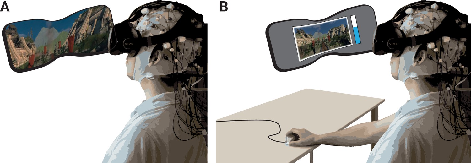
Schematic of experimental setup.

(A) The participants underwent the experience (two rollercoasters separated by a break) in immersive virtual reality (VR), while EEG was recorded. (B) They then continuously rated the level of emotional arousal with a dial viewing a replay of their experience. The procedure was completed twice, without and with head movements.

Procedure

Request a detailed protocol

Participants came to the lab and filled in the pre-test questionnaires. After the torso and limb electrodes had been attached, participants completed a heartbeat guessing task (Schandry, 1981) to assess inter-individual differences in interoceptive accuracy (the results of peripheral physiology and interoception will be reported elsewhere). Then, the EEG cap was attached, and the HMD was carefully placed on top of it. To prevent or minimize (e.g., movement-related) artefacts, customized cushions were placed below the straps of the VR headset to reduce the contact with the EEG sensors. In addition, the VR experience took place while seated and without full body movements (participants were asked to keep their feet and arms still during the recordings). A white grid was presented in the HMD to ensure that the participants’ vision was clear. They then completed a 10 min resting-state phase (5 min eyes open, 5 min eyes closed), before experiencing the first VR episode, which consisted of the two virtual rollercoaster rides and the intermediate break: first the ‘Space’ and then, after the break, the ‘Andes’ rollercoaster. In the subsequent rating phase, they recalled and continuously rated their emotional arousal while viewing a 2D recording of their experience. Importantly, each participant completed the VR episode (plus rating) twice: once while not moving the head (nomov condition) and once while freely moving the head (mov condition) during the VR experience. The sequence of the movement conditions was counterbalanced across participants (n = 19 with nomov condition first). At the end of the experiment, participants completed two additional questionnaires (the SUS and the questionnaire on subjective feelings of presence and valence during the virtual rollercoaster rides) before they were debriefed.

Data analysis

Request a detailed protocol

To exclude effects related to the on- or offset of the rollercoasters, data recorded during the first and the last 2.5 s of each rollercoaster were removed and the inter-individually slightly variable break was cropped to 30 s. The immersive VR experience that was analysed thus consisted of two time series of 270 s length each per participant (nomov and mov).

Self-reports

Questionnaires

Request a detailed protocol

Inter-individual differences as assessed by the trait questionnaires were not the focus of this study, and their results (together with the peripheral physiological and interoception data) will be reported elsewhere. The sum of the simulator sickness ratings before and after the experiment was compared using a two-sided paired t-test.

Emotional arousal

Request a detailed protocol

Emotional arousal ratings were resampled to 1 Hz by averaging non-overlapping sliding windows, yielding one arousal value per second. For the classification analyses, ratings were divided by a tertile split into three distinct classes of arousal ratings (low, medium, high) per participant. For the binary classification (high vs. low arousal), the medium arousal ratings were discarded.

Neurophysiology

Preprocessing

Request a detailed protocol

EEG data were preprocessed and analyzed with custom MATLAB (RRID:SCR_001622) scripts built on the EEGLAB toolbox (RRID:SCR_007292, v13.5.4b; Delorme and Makeig, 2004). The preprocessing steps were applied separately for data recorded during the nomov and mov conditions (i.e., without and with head movement). Continuous data were downsampled to 250 Hz (via the ‘pop_resample.m’ method in EEGLAB) and PREP pipeline (v0.55.2; Bigdely-Shamlo et al., 2015) procedures were applied for detrending (1 Hz high-pass filter, Hamming windowed zero-phase sinc FIR filter, cutoff frequency (–6 dB): 0.5 Hz, filter order: 827, transition band width: 1 Hz), line-noise removal (line frequency: 50 Hz), robust referencing to average, and detection as well as spherical interpolation of noisy channels. Due to the relatively short lengths of the time series, the default fraction of bad correlation windows (parameter ‘badTimeThreshold’, used to mark bad channels) was increased to 0.05. For all other parameters, default values of PREP were kept. On average, 2.08 and 2.47 channels per subject were interpolated in the nomov and mov condition, respectively. Data remained high-pass filtered for the further steps of the analysis. Retrospective arousal ratings were added to the data sets, labelling each second of data with an associated arousal rating used as target for the later classification and regression approaches.

ICA decomposition was used to identify and remove EEG artefacts caused by eye movements, blinks, and muscular activity. To facilitate the decomposition, ICA projection matrices were calculated on a subset of the data from which the noisiest parts had been removed. To this end, a copy of the continuous data was split into 270 epochs of 1 s length. Epochs containing absolute voltage values > 100 µV in at least one channel (excluding channels that reflected eye movements, i.e., EOG channels, Fp1, Fp2, F7, F8) were deleted. Extended infomax (Lee et al., 1999) ICA decomposition was calculated on the remaining parts of the data (after correcting for rank deficiency with a principal component analysis). Subjects with >90 to-be-deleted epochs (33% of the data) were discarded from further analyses (nomov: n = 5; mov: n = 10). Artefactual ICA components were semi-automatically selected using the SASICA extension (Chaumon et al., 2015) of EEGLAB and visual inspection. On average, 13.41 (nomov) and 10.31 (mov) components per subject were discarded. The remaining ICA weights were back-projected onto the continuous time series.

Dimensionality reduction: SSD in the (individual) alpha frequency range

Our main hypothesis was that EEG-derived power in the alpha frequency range allows the discrimination between different states of arousal. To calculate alpha power, we adopted spatio-spectral decomposition (SSD; Nikulin et al., 2011) which extracts oscillatory sources from a set of mixed signals. Based on generalized eigenvalue decomposition, it finds the linear filters that maximize the signal in a specific frequency band and minimize noise in neighbouring frequency bands. Preprocessing with SSD has been previously shown to increase classification accuracy in BCI applications (Haufe et al., 2014a). The alpha frequency range is typically fixed between 8 and 13 Hz. The individual alpha peak frequency, however, varies intra- and inter-individually, for example, with age or cognitive demand (Haegens et al., 2014; Mierau et al., 2017). To detect each participant’s individual peak of alpha oscillations for the SSD, (1) the power spectral density (PSD) of each channel was calculated using Welch’s method ( $s e g m e n t l e n g t h = 5 s * s a m p l i n g f r e q u e n c y$ [i.e., 250 Hz] with 50% overlap) in MATLAB (pwelch function). (2) To disentangle the power contribution of the 1/f aperiodic signal from the periodic component of interest (i.e., alpha), the MATLAB wrapper of the FOOOF toolbox (v0.1.1; Haller et al., 2018; frequency range: 0–40 Hz, peak width range: 1–12 Hz, no minimum peak amplitude, threshold of two SDs above the noise of the flattened spectrum) was used. The maximum power value in the 8–13 Hz range was considered the individual alpha peak frequency α_i, on which the SSD bands of interest were defined (bandpass signal α_i ± 2 Hz, bandstop noise α_i ± 3 Hz, bandpass noise α_i ± 4 Hz).

The entire procedure was separately applied to the nomov and the mov condition to account for potential peak variability (Haegens et al., 2014; Mierau et al., 2017). SSD was then computed based on these peaks. A summary of the resulting individual alpha peak frequencies can be found in Figure 2—source data 1. Figure 2 shows the averaged power spectrum across all participants and electrodes. A clearly defined peak in the alpha frequency range is discernible for both conditions (nomov, mov) as well as for states of high and low emotional arousal.

Figure 2

Download asset Open asset

Group averaged power spectra for the two emotional arousal levels (low, high) and head movement conditions (nomov, mov).

Thick lines represent the mean log-transformed power spectral density of all participants and electrodes. Shaded areas indicate the standard deviation of the participants. High and low emotional arousal are moments that have been rated as most (top tertile) and least arousing (bottom tertile), respectively (the middle tertile was discarded; see main text). The power spectra were produced using MATLAB’s *pwelch* function with the same data (after ICA correction and before spatio-spectral decomposition [SSD] filtering) and parameters as the individual alpha peak detection (see Materials and methods section for details). A tabular overview of the alpha peak frequencies of the individual participants is available as Figure 2—source data 1.

Figure 2—source data 1 Selected alpha peaks (8–13 Hz) per participant and condition. Results of FOOF computations for three different conditions: eyes-closed resting state, nomov, and mov.: https://cdn.elifesciences.org/articles/64812/elife-64812-fig2-data1-v2.csv
Download elife-64812-fig2-data1-v2.csv

SSD components selection

Request a detailed protocol

The SSD components with sufficient alpha information (i.e., power in the alpha frequency range that exceeds the noise level) were selected with the following steps (see Figure 3):

Figure 3

Download asset Open asset

Schematic of the selection of individual alpha components using spatio-spectral decomposition (SSD).

(*Left*) 1/f estimation (dotted grey line) to detrend SSD components (solid turquoise line). (*Right*) After detrending the signal, components were selected, whose peak in the detrended alpha window (centred at the individual alpha peak, vertical dotted grey line) was (A) > 0.35 V²/Hz (indicated by horizontal dotted red line) and (B) higher than the bigger of the two mean amplitudes of the adjacent frequency flanks (2 Hz width).

The PSD of a component was calculated using Welch’s method ( $s e g m e n t l e n g t h = 5 s * s a m p l i n g f r e q u e n c y$ [i.e., 250 Hz] with 50% overlap) implemented in SciPy (RRID:SCR_008058, v1.4.1; Jones et al., 2001).
The 1/f curve was fitted in the signal range between 0 and 40 Hz, excluding a ± 4 Hz window around the individual alpha peak frequency α_i of the subject i. The 1/f curve was defined (in log scale) as $f^{- 1} = l o g (\frac{1}{a \cdot x^{b}})$ , where x is the given component in the frequency domain, $a$ serves as stretch parameter, and $b$ represents the slope of the 1/f curve.
After fitting these parameters, the signal was detrended with respect to the estimated 1/f curve.
Those components were selected, whose alpha peak power in the detrended alpha window (as defined in (1)) was (A) greater than zero plus a decision threshold, which was set to 0.35 $\frac{μ V^{2}}{H z}$ , and (B) higher than the mean amplitude of the adjacent frequency flanks of 2 Hz width on both sides of the window, that is, $p o w e r (a l p h a p e a k) - (m e a n p o w e r (f l a n k)) \geq 1.45 S D$ (after z-scoring the detrended signal). The two criteria guaranteed the selection of components with a clearly defined alpha-amplitude peak over the noise-threshold defined by $f^{- 1}$ (see Figure 3).

Particularly the combination of SSD with narrow-band filtering in the alpha-frequency range lowers the probability of signal contamination elicited by artefact-related oscillations, which are typically strongest in frequency ranges above (e.g., muscular activity; Muthukumaraswamy, 2013) or below the alpha band (e.g., skin potentials, Kappenman and Luck, 2010, or eye blinks, Manoilov, 2007; for a comprehensive overview, see also Chaumon et al., 2015). Decoding models (SPoC, CSP, LSTM; described below) were trained on those subjects with at least four selected SSD components (26 in the nomov and 19 in the mov). On average, 7.63 of 18.81 (40.53 %) in the nomov and 5.63 of 15.22 (36.98 %) SSD components were selected in the mov condition. Importantly, SSD components had spatial topographies corresponding to occipito-parietal and fronto-central source locations, thus covering brain areas previously implicated in emotional arousal and its regulation.

Source power comodulation

Request a detailed protocol

To test the hypothesis that alpha power in the EEG negatively covaries with the continuous level of subjective emotional arousal, SPoC (as described in Dähne et al., 2014; NB: throughout the paper, ‘SPoC’ refers to SPoC_λ) was applied to EEG data composed of the selected SSD components and filtered around the central individual alpha peak. Formally, SPoC is an extension of CSP (see below) for regression-like decoding of a continuous target variable. The information contained in the target variable is used to guide the decomposition of neural components that is correlated or anti-correlated with it (Dähne et al., 2014). SPoC has been shown to outperform more conventional approaches to relate neural time series to continuous behavioural variables (e.g., correlating power extracted in sensor space and/or after blind source separation methods), which also suffer from additional drawbacks (e.g., lack of patterns’ interpretability and lack of adherence to the M/EEG generative model; for details, see Dähne et al., 2014). The supervised decomposition procedure takes the variable z as target, which comprises the continuous arousal ratings (normalized and mean-centred; 270 s per participant). To reach the same temporal resolution as z (i.e., 1 Hz), EEG data were epoched into 270 consecutive segments of 1 s length. For a specific epoch $(e)$ , the power of an SPoC component ( $\hat{s} = W^{T} X$ , where $W^{T}$ corresponds the transpose of the unmixing matrix $W$ and $X$ to the data matrix of $e$ in SSD space) can be approximated by the variance of its signal within that time interval ( $V a r [\hat{s}] (e)$ ; Dähne et al., 2014). SPoC was separately applied to each participant, producing a number of components equal to the number of previously selected SSD components. The stability and significance of the extracted components was tested with a permutation approach (1000 iterations): z values were shuffled to create a surrogate target variable with randomized phase but same auto-correlation (Theiler et al., 1992; adapted from the original SPoC function: https://github.com/svendaehne/matlab_SPoC/blob/master/SPoC/spoc.m; Dähne, 2015, Dähne et al., 2014). In accordance with the primary objective of SPoC to reconstruct the target variable z, lambda values (λ, i.e., optimization criterion of SPoC: component-wise covariance between z and alpha power; sorted from most positive to most negative) and corresponding Pearson correlation values (r) between z and the estimated z_est (obtained via $z_{e s t} = V a r [W^{(i) T} X] (e)$ ) were then calculated for each iteration to generate a naive probability density function (i.e., null hypothesis distribution) and to estimate the probability that the correlation value that was calculated with the original target variable z was obtained by chance. Of note, z_est denotes the power time course of the spatially filtered signal that maximally covaries with the behavioural variable z. Depending on i (i.e., from which side of the SPoC unmixing matrix the component is chosen), z_est will be (maximally) positively (left side of the matrix) or (maximally) negatively (right side of the matrix) correlated with z. Given our main hypothesis of an inverse relationship between alpha power and self-reported emotional arousal, we therefore only retained, for each participant, the component with the most negative (precisely: ‘smallest’) lambda value λ (disregarding the p-value to avoid circularity; Kriegeskorte et al., 2009), corresponding to the last column of the unmixing matrix $W$ .

In line with our hypothesis, single participants’ p-values were then obtained by computing the number of permuted r values that were smaller than the one estimated with SPoC.

Crucially, since the extracted linear spatial filters $W$ cannot be directly interpreted (Haufe et al., 2014b), topographical scalp projection of the components are represented by the columns of the spatial patterns matrix $A$ obtained by inverting the full matrix $W$ (Figure 6).

Common spatial patterns

Request a detailed protocol

To further test the hypothesis of a link between alpha power and subjective emotional arousal, we aimed to distinguish between the most and the least arousing phases of the experience by using features of the alpha bandpower of the concurrently acquired EEG signal. We followed an approach which has successfully been used in BCI research to discriminate between event- or state-related changes in the bandpower of specific frequency ranges in the EEG signal: the common spatial patterns algorithm specifies, by means of a generalized eigenvalue decomposition, a set of spatial filters to project the EEG data onto components whose bandpower maximally relates to the prevalence of one of two dichotomous states (Blankertz et al., 2008; Ramoser et al., 2000). In our case, we were interested in distinguishing moments that had been rated to be most (top tertile) and least arousing (bottom tertile).

Using the EEGLAB extension BCILAB (RRID:SCR_007013, v1.4-devel; Kothe and Makeig, 2013), data of the selected SSD components, bandpass filtered around the individual alpha peak ±2 Hz, were epoched in 1 s segments. This sample length was chosen to enable the extraction of neural features and corresponding changes in the subjective experience, while maximizing the number of samples from the sparse datasets. Epochs with mid-level arousal ratings (middle tertile) were discarded, yielding 180 epochs (90 per class) for each subject (per movement condition). To assess the classification performance, a randomized 10-fold cross-validation procedure, a common solution for sparse training data (Bishop, 2006), was used. Per fold, a CSP-based feature model was calculated on the training data by decomposing the signal of the selected SSD components according to the CSP algorithm. A feature vector comprising the logarithmized variance of the four most discriminative CSP components (using two columns from each side of the eigenvalue decomposition matrix as spatial filters) was extracted per epoch. Data from the training splits were used to train a linear discriminant analysis (LDA) on these feature vectors (Fisher, 1936). Covariance matrices used for calculating the LDA were regularized by applying the analytic solution implemented in BCILAB (Ledoit and Wolf, 2004). The LDA model was then used to classify the feature vectors extracted from the epochs in the test split to predict the according arousal label. Average classification accuracy (defined as $1 - m i s c l a s s i f i c a t i o n r a t e$ ) over the 10 folds was taken as the outcome measure to assess the predictive quality of the approach. To allow a spatial interpretation of the projections, like with the SPoC components, the spatial patterns of the two most extreme CSP components (associated with the largest and smallest eigenvalue) that were used to calculate the feature vectors for the linear classification were plotted in Figure 6 (normalized and averaged across subjects per condition) and Figure 6—figure supplement 1 (per single subject and condition). Source localized patterns are shown in Figure 9.

Sub-blocked cross-validation

Request a detailed protocol

For non-stationary, auto-correlated time-series data, randomized cross-validation can inflate the decoding performance (Roberts et al., 2017). To assess and minimize this possibility, we tested whether a blocked cross-validation, which preserves temporal neighbourhood structures among samples, changes the classification results of the CSP analysis. To ensure balanced classes in the training set, the ‘synthetic minority oversampling technique’, which oversamples the less frequently represented class, was applied (Chawla et al., 2002; as implemented in Larsen, 2021). The test set was left unbalanced as oversampling of test data can invalidate the assessment of model performance (Altini, 2015), and the area under the curve of the receiver operating characteristic (ROC-AUC) was used as a performance measure. To avoid homogeneous test sets (i.e., with samples from only one target class), which (1) would occur in many subjects after ‘conventional’ chronological cross-validation and (2) would preclude ROC-AUC calculation, a ‘sub-blocked’ cross-validation was used: for each subject, the dataset was split into three sub-blocks of equal length, which were then used to stratify the data assignment for a (sub-blocked) chronological 10-fold cross-validation. In this design, each fold consists of a concatenation of equally sized stretches of consecutive data samples taken from each of the sub-blocks: for example, to build the validation set in the first fold [x₁, x₂, x₃], with x_i being the n first samples from the ith sub-block where n is the total number of samples in the dataset divided by 10 * 3 (number of folds * number of sub-blocks). Thereby the temporal neighbourhood structure among data samples is largely preserved when splitting them into training and testing sets. The (smaller) test set is still sampled from different parts of the experience, which decreases the risk of obtaining homogeneous test sets (e.g., only ‘low arousing’ sections).

Source localization

Request a detailed protocol

Exact low-resolution tomography analysis (eLORETA, RRID:SCR_007077; Pascual-Marqui, 2007) was used to localize the sources corresponding to the component extracted via SPoC and CSP. Our pipeline was based on the work of Idaji et al., 2020, who customized the eLORETA implementation of the M/EEG Toolbox of Hamburg (https://www.nitrc.org/projects/meth/).

Our forward model was constructed via the New York Head model (Haufe et al., 2014b; Haufe and Ewald, 2019; Huang et al., 2016) with approximately 2000 voxels and by using 28 out of 30 scalp electrodes (TP9 and TP10 were removed because they are not contained in the model). Crucially, we focused on dipoles perpendicular to the cortex. eLORETA was then used to construct a spatial filter for each voxel from the leadfield matrix, and respective sources were computed by multiplying the resultant demixing matrix with the spatial patterns $A$ of the selected SPoC and CSP components. Inverse modelling was computed separately per participant and condition before it was averaged for each condition across all subjects (Figure 9).

LSTM RNN

Request a detailed protocol

Deep learning models have become a useful tool to decode neural information (e.g., Agrawal et al., 2014; Khaligh-Razavi and Kriegeskorte, 2014). Applying a deep learning approach to the time series of EEG recordings (e.g., Bashivan et al., 2016) can be achieved using LSTM RNNs (Hochreiter and Schmidhuber, 1995; Hochreiter and Schmidhuber, 1997). With their property to store and control relevant information over time, they can find adjacent as well as distant patterns in (time) sequential data. The LSTM analysis was implemented in the Python-based (RRID:SCR_008394) deep learning library TensorFlow (RRID:SCR_016345, v1.14.0; Google Inc, USA; Abadi et al., 2015; Zaremba et al., 2015).

Model architecture and hyperparameter search

Request a detailed protocol

Deep learning models usually have a high variance due to random weight initialization, architectural choices, and hyperparameters (HPs; Geman et al., 1992; but see Neal et al., 2019). We here used a two-step random search (Bergstra and Bengio, 2012) strategy in order to find optimal HPs, to reduce the model variance and make the search computationally feasible. First, a broad random search was applied on a random subset of 10 subjects (20 random combinations) in each condition. Then, the two best HPs per subject were taken and applied to the datasets of all subjects. Due to time constraints and computational complexity, the HP search was limited to a predefined range of settings and the model architecture was constrained to maximal two LSTM layers followed by maximal two fully connected layers (FC; Hefron et al., 2017; see Figure 4). Each layer size ls_l varied between 10 and 100 nodes (ls_l ∈ 10, 15, 20, 25, 30, 40, 50, 65, 80, 100), and a successive layer needed to be equal or smaller in size (bottleneck architecture). The output of each layer was squashed through either rectified linear units or exponential linear units, which both allow for steeper learning curves in contrast to conventional activation functions such as sigmoid nonlinearity (Clevert et al., 2016). The output of the last network layer (FC_L) was fed into a tangens hyperbolicus (tanh) to match the binned ratings, which were labelled with –1 or 1, respectively. We applied a mean-squared error loss to calculate the difference between the model output (i.e., the prediction) and the labels, leading to a stronger weighting of losses at the upper- or lower-class border, respectively. To control and tax too large model weights, different regularization methods (L1, L2) with different regularization strengths (Λ ∈ 0.00, 0.18, 0.36, 0.72, 1.44) were tested. Weights were optimized using Adam (learning rate: lr ∈ 1e^–2, 1e^–3, 5e^–4) due to its fast convergence (Marti, 2015; see also Ruder, 2017). The number of input components (SSD, N_comp: N ∈ [1, 10]) was treated as HP. The specific N_comp neural components were successively drawn according to the order of the SSD selection.

Figure 4

Download asset Open asset

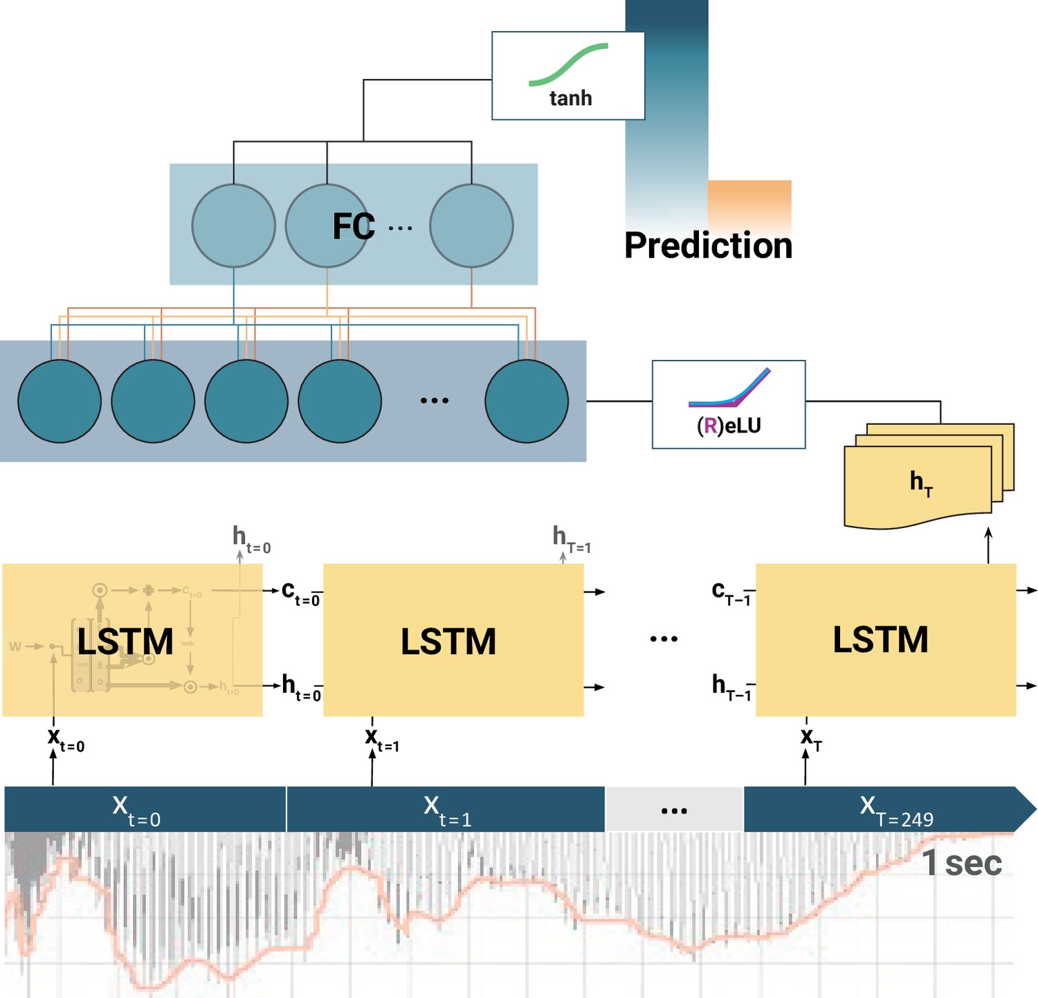
Schematic of the long short-term memory (LSTM) recurrent neural network (RNN).

At each training step, the LSTM cells successively slide over 250 data arrays of neural components (x_t=0, x_t=1,..., x_T=249) corresponding to 1 s of the EEG recording. At each step t, the LSTM cell computes its hidden state *h_t*. Only the final LSTM output (*h_T*) at time-step T = 249 is then fed into the following fully connected (FC) layer. The outputs of all (LSTMs, FCs) but the final layer are normalized by rectified linear units (ReLU) or exponential linear units (ELU). Finally, the model prediction is extracted from the last FC layer via a tangens hyperbolicus (*tanh*). Note: depending on model architecture, there were one to two LSTM layers, and one to two FC layers. The hyperparameter constellations that yielded the highest accuracy for the individual participants per movement condition are available as Figure 4—source data 1.

Figure 4—source data 1 Long short-term memory (LSTM) hyperparameter search per movement condition. LSTM: number of cells per layer. FC: number of hidden units in fully connected layer, before final output neuron. l.rate: learning rate. reg.: type of weight regularizer. reg. strength: respective regularization strength. activ.func: intermediate layer activation function. components: individually selected components for training after spatio-spectral decomposition (SSD) selection.: https://cdn.elifesciences.org/articles/64812/elife-64812-fig4-data1-v2.zip
Download elife-64812-fig4-data1-v2.zip

Training procedure

Request a detailed protocol

The final dataset per subject was a three-dimensional tensor of size 270 × 250 × 10 (epochs × samples × components). If less than 10 components were extracted for a given subject, the tensor was filled with zero vectors. After some test runs and visual observation of the convergence behaviour of the learning progress, training iterations were set to 20 (i.e., the model ran 20 times through the whole training dataset). The 1 s samples were fed into the LSTM in random mini-batches of size 9 (bs = 9), since training on batches allows for faster and more robust feature learning (Ruder, 2017), leading to the following input tensor at training step ts: $x_{t r a i n, t s}^{b s x 250 x 10}$ .

Statistical evaluation

Request a detailed protocol

To test whether the results of the binary modelling approaches (CSP, LSTM) were statistically significantly above chance level, exact binomial tests were conducted per subject and experimental condition (nomov, mov) over all 180 epochs of the respective time series (nomov, mov). To do so, for each of the binary modelling approaches (CSP, LSTM), the predictions for the single epochs in the 10 test splits of the cross-validation were concatenated to a single vector. The proportion of correct and false predictions was then compared to a null model with prediction accuracy 0.5 (chance level). To test the average (across subjects) classification accuracies of the binary models, we calculated one-sided one-sample t-tests, comparing the mean accuracy of the respective model for both experimental conditions against the theoretical prediction accuracy of a random classifier (0.5). To test whether classification accuracies differed between the two models (CSP, LSTM) or between the experimental conditions (nomov, mov), a repeated-measures two-way ANOVA was conducted on the accuracy scores of all subjects with preprocessed data from both conditions (n = 18).

To account for potential biases due to auto-correlations in the time series which might affect the statistical evaluation of the classification model, in an additional control analysis, block permutation testing was applied to the CSP approach: to maintain a local auto-correlative structure similar to the original data in the permuted target vectors, the time series were split into 10 equally sized blocks, which were then shuffled while the internal temporal structure of each block remained intact (Winkler et al., 2014). To test whether the actual decoding scores (from non-permuted data) were significantly above chance level, we assessed their percentile rank in relation to the null distributions (1000 permutations) on the single-subject level. On the group level, one-sided paired t-tests were used to compare the distribution of the actual decoding results against the distribution of the means of the null distributions per subject. Due to its high computational processing cost and duration, we did not perform permutation testing for the LSTM model.

For SPoC, in addition to the aforementioned within-participants permutation approach yielding a single p-value for each component, group-level statistics were assessed: the hypothesis of a negative correlation between alpha power and emotional arousal was tested with a one-sample, one-tailed t-test on the correlation values between z and z_est, which assessed whether the mean correlation value per condition was significantly lower than the average of the permuted ones.

The code for preprocessing of the data, the three prediction models, and the statistical evaluation is available on GitHub (https://github.com/NeVRo-study/NeVRo; Hofmann et al., 2021; copy archived at swh:1:rev:669d5c2d6c73cbb70422efb933916fe8304195b5).

Control analysis: excluding the break for model training

Request a detailed protocol

The 30 s break differed from the rollercoaster rides in visual features (e.g., static vs. dynamic input) and in arousal ratings, which were constantly relatively low during the break (see Figure 5). Thus, the break contributed mainly to the ‘low arousing’ class. To test whether the decoding approaches also succeed if the break section is excluded from the analysis, SPoC and CSP decoding were repeated for the data without the break, that is, the rollercoasters only (240 s in total). The LSTM approach was skipped in this control analysis due to its computational processing cost and duration, and the comparable performance with CSP in the main analysis. For the classification (CSP), the tertile split on the subjective arousal ratings was recalculated such that the class of ‘low arousal’ segments now comprises the least arousing sections of the rollercoasters. We then trained and tested the SPoC and CSP models with the procedures that were used for the original dataset (incl. the break). For maximal stringency, we used the sub-blocked cross-validation and block permutation approach to assess the performance of the CSP model. To test whether excluding the break changed the model performance, we compared the distributions of the decoding performance parameters (SPoC: Pearson correlation with target; CSP: ROC-AUC) from the data with and without the break using two-sided paired t-tests. We did this per model and movement condition.

Figure 5 with 1 supplement see all

Download asset Open asset

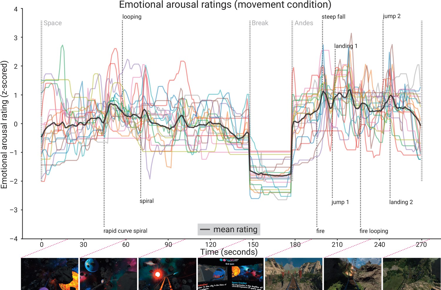
Subjective emotional arousal ratings (movement condition).

Emotional arousal ratings of the experience (with head movement; see Figure 5—figure supplement 1 for the ratings from the no-movement condition). Coloured lines: individual participants; black line: mean across participants; vertical lines (light grey): beginning of the three phases (Space Coaster, Break, Andes Coaster); vertical lines (dark grey): manually labelled salient events (for illustration). Bottom row: exemplary screenshots of the virtual reality (VR) experience. The ratings for the condition without head movement are shown in the figure supplement.

Results

Participants

Forty-five healthy young participants (22 men, M ± SD: 24.6 ± 3.1, range: 20–32 years) completed the experiment. Data from eight participants needed to be discarded due to technical problems (n = 5) or electrode malfunctioning (n = 1); one participant discontinued the experiment and another participant reported having taken psychoactive medication. The data from 37 participants entered the analysis (17 men, age: M ± SD: 25.1 ± 3.1, range: 20–31 years). After quality assurance during the EEG preprocessing, data from 26 participants in the condition with no head movement (nomov) and 19 in condition with free head movement (mov) entered the statistical analyses that included EEG data.

Self-reports

Questionnaires

From before (M ± SD: 8.68 ± 2.82, range: 6–17) to after the experiment (M ± SD: 11.82 ± 5.24, range: 6–29), the overall simulator sickness (e.g., nausea, headache) increased significantly (t(36) = 3.72, p = 0.0007). As the trait questionnaires are not the focus of this study, their results will be reported elsewhere.

Emotional arousal ratings

The retrospective emotional arousal ratings for the VR experience, averaged across all subjects and timepoints, were 46.94 ± 12.50 (M ± SD, range: 16.17–66.29) in the nomov and 50.06 ± 12.55 (M ± SD, range: 18.00–69.94) in the mov condition. Qualitatively, the emotional arousal was highest for the Andes Coaster, lower for the Space Coaster, and lowest for the break (see Figure 5).

Neurophysiology

SPoC

SPoC results showed that for 24/26 (92.30%) participants in the nomov and 16/19 (84.21%) participants in the mov condition (see Figure 10—source data 1 for single-participant results), the component with the highest absolute lambda value corresponded to the one that maximized the negative correlation between z (normalized and mean-centred subjective ratings) and alpha power. Based on permutation-based testing (1000 iterations; exact p values are reported in Figure 10—source data 1), the negative correlation was statistically significant (p < 0.05) in 8/26 (30.76%) participants for the nomov and 7/19 (36.84%) participants for the mov condition. The global mean lambda value of these components was –0.46 for the nomov (range: –1.49 to +0.08) and –0.42 for the mov condition (range: –1.49 to +0.02). The mean Pearson correlation value between the target variable z and z_est (estimated target variable) was significantly lower than the average of single participants’ permuted ones for both the nomov (M ± SD: –0.25 ± 0.12; range: –0.53 to + 0.09; t_nomov(25) = –3.62; p < 0.01) and the mov condition (M ± SD: –0.25 ± 0.12; range: –0.52 to +0.04; t_mov(18) = –3.13; p < 0.01).

CSP

The classifier based on CSP was able to decode significantly above chance level whether a subject experienced high or low emotional arousal during a given second of the experience. On average, the classification accuracy was 60.83% ± 7.40% (M ± SD; range: 47.22–77.78%) for the nomov, and 60.76% ± 6.58% (M ± SD; range: 48.33–71.67%) for the mov condition. Both were significantly above chance level (t_nomov(25) = 7.47, p_nomov < 0.001; t_mov(18) = 7.12, p_mov < 0.001). At the single-subject level, the classification accuracy was significantly above chance level (p < 0.05) for 17/26 (65.38%) participants in the nomov, and for 12/19 (63.16%) participants in the mov condition (see Figure 10—source data 1 for single-participant results). The spatial patterns yielded by the CSP decomposition are shown in Figure 6 (across participants) and in Figure 6—figure supplement 1 (individual participants). Corresponding alpha power sources (located via eLORETA) are shown in Figure 9.

Figure 6 with 1 supplement see all

Download asset Open asset

Spatial patterns resulting from spatio-spectral decomposition (SSD), source power comodulation (SPoC), and common spatial pattern (CSP) decomposition.

Colours represent absolute normalized pattern weights (inverse filter matrices) averaged across all subjects per condition (nomov: without head movement, mov: with head movement). Before averaging, the pattern weight vectors of each individual subject were normalized by their respective L2-norm. To avoid cancellation due to the non-polarity-aligned nature of the dipolar sources across subjects, the average was calculated from the absolute pattern weights. SSD allows the extraction of components with a clearly defined spectral peak in the alpha frequency band. Shown are the patterns associated with the four SSD components that yielded the best signal-to-noise ratio (*left column*). The SSD filtered signal was the input for the decoding approaches SPoC, CSP, and LSTM: SPoC adds a spatial filter, optimizing the covariance between the continuous emotional arousal ratings and alpha power. Shown here is the pattern of the component which – in line with our hypothesis – maximized the inverse relationship between emotional arousal and alpha power. CSP decomposition yielded components with maximal alpha power for low-arousing epochs and minimal for high-arousing epochs (*bottom row in the CSP panel*) or vice versa (*upper row in the CSP panel*). The high correspondence between the patterns resulting from SPoC and CSP seems to reflect that both algorithms converge to similar solutions, capturing alpha power modulations in parieto-occipital regions as a function of emotional arousal. The spatial patterns for the individual subjects are displayed in the figure supplement. (Note: as the LSTM results cannot be topographically interpreted, they are not depicted here.)

To test for potential biases from the model or the data, specifically its auto-correlative properties, we ran a control analysis for CSP using sub-blocked chronological cross-validation and block permutation for statistical evaluation on the single-subject level.

Also under these – more strict – evaluation criteria, the average decoding performance (ROC-AUC) for CSP was significantly above chance level, both in the nomov (ROC-AUC: 0.61 ± 0.09 M ± SD, range: 0.42–0.79; t(25) = 4.59, p < 0.001) and in the mov condition (ROC-AUC: 0.60 ± 0.09 M ± SD, range: 0.44–0.74; t(18) = 3.27, p < 0.01). On the single-subject level (as assessed by permutation tests), decoding performance was significantly (p < 0.05) higher when decoding the actual, unpermuted labels compared to the block-permuted labels for 9/26 (34.62%) participants in the nomov and 5/19 (26.32%) participants in the mov condition.

LSTM

After a random search over a constrained range of HPs, we extracted the best individual HP set per subject (see Figure 4—source data 1 for the list of best HPs per condition). The mean classification accuracy was 59.42% ± 4.57% (M ± SD; range: 52.22–68.33%) for the nomov, and 61.29% ± 4.5 % (M ± SD; range: 53.89–71.11%) for the mov condition. Both were significantly above chance level (t_nomov(25) = 10.82, p_nomov < 0.001; t_mov(16) = 10.51, p_mov < 0.001). At the single-subject level, the classification accuracy was significantly above chance level for 16/26 (61.54%) participants in the nomov condition, and for 16/19 (84.21%) participants in the mov condition (same test as for CSP results; see Figure 10—source data 1).

Comparison of model performances

As an illustration of the prediction behaviour across all three models in one participant (with high performance for all three decoding approaches), see Figure 7. Correlations of performances across models and experimental conditions are shown in Figure 10. The (positive) correlation between the two binary classification approaches (CSP, LSTM) was significant (after Bonferroni multiple-comparison correction), irrespective of the experimental condition (nomov, mov), meaning that subjects who could be better classified with CSP also yielded better results in the LSTM-based classification. In a repeated-measures ANOVA testing for differences in the accuracies of the two binary classification models (CSP, LSTM) and the two conditions (nomov, mov), none of the effects was significant: neither the main effect model (F(1,17) = 0.02, p = 0.904) nor the main effect condition (F(1,17) = 0.72, p = 0.408) or their interaction (F(1,17) = 1.59, p = 0.225). For a further comparison of the performances of the classification approaches, the respective confusion matrices are depicted in Figure 8 (average across the subjects per condition and model).

Figure 7

Download asset Open asset

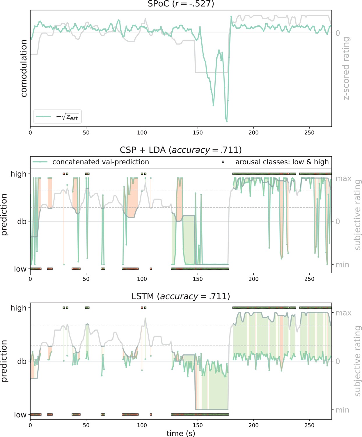
Exemplary model predictions.

Predictions (turquoise line, dots) across models trained on the data of one participant in the movement condition (source power comodulation [SPoC]: normalized negative *z_est, here comodulation;* common spatial patterns [CSP]: posterior probability; long short-term memory [LSTM]: *tanh* output). *Top row*: most negatively correlating SPoC component (for visualization we depict the normalized and mean-centred value of the rating and of the negative square root of z_est). *Middle and lower row*: model predictions on validation sets (across the cross-validation splits) for CSP and LSTM, respectively. The grey curvy line in each panel indicates the continuous subjective rating of the participant. Horizontal dotted lines indicate the class borders. The area between these lines is the mid-tertile which was discarded for CSP and LSTM analyses. Class membership of each rating sample (1 s) is indicated by the circles at the top and bottom of the rating. A model output falling under or above the decision boundary (db) indicates the model prediction for one over the other class, respectively. The correct or incorrect prediction is indicated by the colour of the circle (green and red, respectively), and additionally colour-coded as area between model output (turquoise) and rating.

Figure 8

Download asset Open asset

Comparison of the binary decoding approaches.

Confusion matrices of the classification accuracies for higher and lower self-reported emotional arousal using long short-term memory (LSTM) (*lower row*) and common spatial patterns (CSP) (*upper row*) in the condition without (*left column*) and with (*right column*) head movement. The data underlying this figure can be downloaded as Figure 8—source data 1.

Figure 8—source data 1 Prediction tables of the binary decoding models. The zip file contains a folder for each of the movement conditions (with and without head movements) with subfolders for the binary decoding approaches (common spatial patterns [CSP], long short-term memory [LSTM]). Each folder includes three types of tables with the same format (Subjects × Samples). Subjects (N varies by condition) who went into the final classification (after removals during preprocessing). Samples (N = 270) refer to the sequential seconds of the experience (total length: 270 s). Each cell contains: targetTable: the target/ground truth assigned to this sample (by binning the continuous rating). CSP: 1=Low Arousal, 2=High Arousal, NaN = Medium Arousal; LSTM: –1=Low Arousal, 1=High Arousal, 0=Medium Arousalprediction. TableProbabilities: the probability/certainty of this sample to be classified as ‘High Arousing’ (positive probabilities) or ‘Low Arousing’ (negative probabilities). predictionTable: the binarized version of the probabilities. CSP: 1=High Arousal, 0=Low Arousal, NaN = Medium Arousal, LSTM: 1=High Arousal, –1=Low Arousal, 0=Medium Arousal.: https://cdn.elifesciences.org/articles/64812/elife-64812-fig8-data1-v2.zip
Download elife-64812-fig8-data1-v2.zip

Control analysis: excluding the break from model training

SPoC and CSP performed significantly above chance level also when trained and tested on data without the break section.

For CSP on data without the break, the average classification performance (ROC-AUC) was 0.57 ± 0.10 (M ± SD; range: 0.28–0.78) in the nomov and 0.59 ± 0.09 (M ± SD; range: 0.45–0.77) in the mov condition (see previous paragraph for the decoding performance with the break included). Average model performances were still significantly above chance level (means of the block permutation distributions on the single-subject level) in both movement conditions (nomov: t(25) = 2.89, p < 0.01; mov: t(18) = 3.50, p < 0.01). On the single-subject level, the classification performance was significantly above chance level for 3/26 (11.54%) participants in the nomov and 5/19 (26.32%) participants in the mov condition.

For SPoC on data without the break, the average Pearson correlation between z and z_est (estimated target variable) was significantly smaller (more negative) than the average of single participants’ permuted correlation values for both the nomov (M ± SD: –0.22 ± 0.08; range: –0.36 to –0.07; t_nomov(25) = –3.17; p < 0.01) and the mov condition (M ± SD: –0.21 ± 0.07; range: –0.37 to –0.061; t_mov(18) = –2.53; p < 0.05). On the single-subject level, 2/26 (7.69%) participants for the nomov and 7/19 (36.84%) participants for the mov condition remained statistically significant (p < 0.05) after permutation-based tests.

Removing the break from the training data overall numerically decreased the decoding performances of both models. For CSP, the decrease was significant in the nomov (t(25) = 2.23, p = 0.034) and not significant in the mov condition (t(18) = 0.57, p = 0.58). For SPoC, the decrease (Pearson correlation) was not significant in both conditions (nomov: t(25) = –1.66, p = 0.108; mov: t(18) = –1.13, p = 0.269).

Discussion

The general aim of this study was to capture the dynamic relationship between subjective experience and neurophysiology under naturalistic stimulation using immersive VR. The hypothesized link between EEG alpha power and self-reported emotional arousal could be confirmed by relating alpha power components to continuous retrospective ratings of emotional arousal (using SPoC) as well as by decoding states of higher and lower emotional arousal from them (using CSP and LSTMs), particularly in parieto-occipital regions. In addition to extending our knowledge about the functional anatomy of emotional arousal, these findings support previous results from classical studies and confirm them under more naturalistic conditions. They thereby pave the way for real-world scenarios and applications.

Physiological and psychological concomitants of emotional arousal

In studies with event-related stimulation or block designs, more emotionally arousing compared to less emotionally arousing images, videos, and sounds were associated with event-related decreases in alpha power, predominantly over parieto-occipital electrodes (De Cesarei and Codispoti, 2011; Luft and Bhattacharya, 2015; Schubring and Schupp, 2019; Uusberg et al., 2013; Koelstra et al., 2012). While such stimuli provide a high degree of experimental control in terms of low-level properties and presentation timings, the emotional experience and its neurophysiology under event-related stimulation may differ from the emotional experience in real-life settings, which is perceptually complex, multisensory, and continuously developing over time.

Our results provide evidence that the neural mechanisms reflected in modulations of alpha power – particularly in parieto-occipital regions – also bear information about the subjective emotional state of a person undergoing an immersive and emotionally arousing experience. Also fMRI studies have related brain activity in parietal cortices and emotional processing (e.g., Lettieri et al., 2019). Our study thus suggests that findings from event-related, simplified stimulation generalize to more naturalistic (i.e., dynamic and interactive) settings.

Paralleling the idea of emotional arousal being a dimension of ‘core affect’ (Russell and Barrett, 1999) and a psychological primitive that underlies many mental phenomena, also alpha oscillations have been connected to various psychological ‘core processes’: for instance, modulations of alpha power were linked to attention (Van Diepen et al., 2019) and memory (Klimesch, 2012). More generally, neural oscillations in the alpha frequency range were suggested to serve functional inhibition of irrelevant sensory input (Jensen and Mazaheri, 2010; Foster and Awh, 2019) and to code for the location and the timing of task-relevant stimuli (Foster et al., 2017). Such processes can be functionally linked to emotional arousal: during emotionally arousing experiences, preferred and enhanced processing of relevant sensory stimuli (e.g., indicating potential threats) is an adaptive behaviour. In line with this, modulations of alpha oscillations over parietal sensors have been linked to threat processing (Grimshaw et al., 2014). Variations in emotional arousal and alpha power may, thus, have guided attention and memory formation also in our experiment: during particularly arousing parts of the rollercoaster, participants may have directed their attention to specific parts of the visual scene, for example, to foresee the end of the looping. Moreover, our inverse modelling (Figure 9) has also localized arousal-related alpha sources in sensorimotor cortices, which could correspond to somatic experiences typically associated with rollercoasters. Some of the averaged spatial patterns (see Figures 6 and 9) we observed for the SPoC- and CSP-based decoding stronger absolute weights for electrodes above right – as compared to left – cortices. Since we did not hypothesize a lateralization of the alpha effects, we refrained from statistically testing differences between the hemispheres. Similar patterns of right-lateralized alpha oscillations have also been related to arousal in major depression (Metzger et al., 2004; Stewart et al., 2011). However, it is unclear to which extent these effects are specific to arousal, as lateralization of alpha power has also been observed in working-memory (Pavlov and Kotchoubey, 2020) and resting-state studies (Ocklenburg et al., 2019). Our results motivate experimental work that will model the link between emotional arousal and alpha oscillations by systematically varying additional variables (e.g., attention, sensorimotor processing). We argue that studying such relationships in naturalistic settings allows embracing and learning statistical interdependencies that are characteristics of the real world.

Figure 9

Download asset Open asset

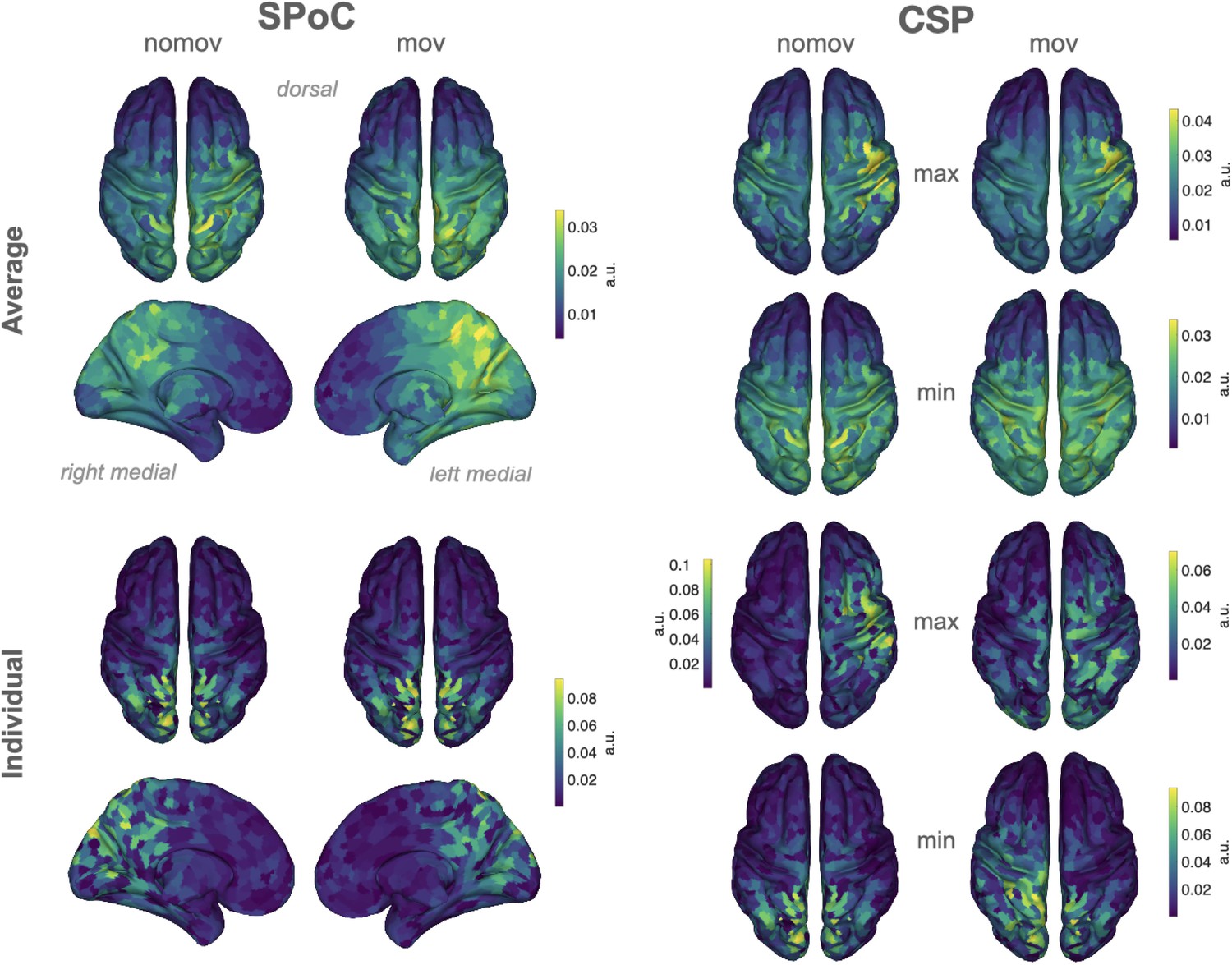
Source reconstructions (exact low resolution tomography analysis [eLORETA]).

The projection of source power comodulation (SPoC) and common spatial patterns (CSP) components in source space confirms the link between emotional arousal and alpha oscillations in parieto-occipital regions. Colours represent the inversely modelled contribution of the cortical voxels to the respective spatial pattern yielded by SPoC or CSP (max: component maximizing power for epochs of high arousal; min: component minimizing power for epochs of high arousal). We applied the same normalization and averaging procedures as for the topoplots in Figure 6. *Upper row*: averaged across all subjects per condition (nomov, mov). *Lower row*: patterns of one individual (the same as in Figure 7).

VR as a step towards a real-world neuroscience

More naturalistic experimental stimulation, for example, using immersive VR, allows to test the brain under conditions it was optimized for and thereby improve the discovery of neural features and dynamics (Gibson, 1978; Hasson et al., 2020). Findings from naturalistic studies can test the real-world relevance of results obtained in highly controlled, abstract laboratory settings (Matusz et al., 2019; Shamay-Tsoory and Mendelsohn, 2019). Challenges of using VR for more naturalistic research designs are the creation of high-quality VR content, more complex technical setups, and discomfort caused by the immersion into the virtual environment (Pan and Hamilton, 2018; Vasser and Aru, 2020). Despite the incongruence between VR rollercoaster-induced visual stimulation and vestibular signals, which may lead to motion sickness (Reason and Brand, 1975), only one of our participants stopped the experiment because of cybersickness. This low number may result from the relatively short length of the VR experience (net length: <20 min) and the professionally produced VR stimulation. Shorter exposure times (Rebenitsch and Owen, 2016) and experiences that elicit stronger feelings of presence have been associated with lower levels of cybersickness (Weech et al., 2019).

Combining EEG with VR provides additional challenges: the signal-to-noise ratio (SNR) can be decreased due to mechanical interference of the VR headset with the EEG cap and due to movement artefacts when the participant interacts with the virtual environment (e.g., head rotations). To ensure high data quality, we applied multiple measures to prevent, identify, reject, or correct artefacts in the EEG signal (see Materials and methods section for details). Ultimately, the performance of all three decoding models did not differ significantly for both conditions (nomov, mov). We suggest that, with appropriate quality assurance during data acquisition and analysis (leading to more data rejection/correction for mov than for nomov), EEG can be combined with immersive VR and free head movements. Other studies of mobile brain imaging, even recording outdoors and with full-body movements, came to similar conclusions (Debener et al., 2012; Ehinger et al., 2014; Gramann et al., 2011; Symeonidou et al., 2018).

Evaluating EEG data from naturalistic experiments using complementary methods

Each of the applied decoding approaches allows for different insights and interpretations, but overall, they yield converging results.

SPoC and CSP

SPoC and CSP share advantages that are common to most spatial filtering methods based on generalized eigenvalue decomposition, namely precise optimization policies, high speed, and interpretability. As dimensionality reduction techniques, they combine data from multiple M/EEG channels to obtain a new signal (component) with a higher SNR (Lotte et al., 2018; Parra et al., 2005). This aids maximizing the difference in the signal of interest between experimental conditions (de Cheveigné and Parra, 2014; Rivet et al., 2009) or against signals in the neighbouring frequency ranges (Nikulin et al., 2011). The similarity between the two approaches (SPoC, CSP) and their interpretability becomes apparent in the resulting spatial patterns: the normalized and averaged SPoC topoplots and source localizations in both conditions (nomov, mov) resemble the ones extracted via CSP to maximize power for the low-arousal epochs of the experience (Figures 6 and 9). SPoC and CSP solve a similar problem here: extracting components whose power is minimal during states of high emotional arousal and maximal during states of low arousal.

This indicates that SPoC and CSP exploited similar spatial informational patterns in the input data. However, the datasets handed to the SPoC and CSP models were not identical. For the CSP analysis, only the upper and lower extreme of the arousal ratings were included (i.e. two-thirds of the data), while epochs with medium arousal ratings (i.e., one-third of the data) were excluded, whereas SPoC was trained on the full continuous data stream. There are two potential explanations for the observation that SPoC and CSP nevertheless yield similar spatial patterns: either the most relevant information was encoded in the most extreme parts of the experience, or there is a truly linear relationship between alpha power and emotional arousal that can be queried on all parts of this spectrum ranging from low to high emotional arousal.

The spatial patterns for the components gained from SSD, SPoC, and CSP exhibit discernible variance between the single subjects (see Figure 6—figure supplement 1). This can be, for example, caused by physiological differences (e.g., different shapes of the skull, different cortical folding) or slightly different positioning of the EEG electrodes. The same cortical source might thereby lead to different patterns of scalp EEG in different participants. Spatial filtering procedures inverse this projection and the extracted patterns therefore also vary across subjects. Such inter-individual differences are well known for BCIs, and extensions for CSP have been suggested, which allow for a transfer of features across subjects (e.g., Cheng et al., 2017). To emphasize the communalities across individual patterns and indicate the cortical areas that contributed most to decoding results, we report the averaged patterns (Figure 6) and the averaged results of the reconstructed cortical sources (Figure 9).

To test for confounds or analytic artefacts, for example, due to auto-correlations in the data, we additionally applied ‘sub-blocked’ cross-validation for model training and block permutation for statistical evaluation. Also under these more strict evaluation conditions, the average decoding performance was significantly above chance level. It is therefore unlikely that the results can be explained solely by dependencies in the data (e.g., auto-correlation) which are not explicitly modelled in the main analysis.

Moreover, to test the impact of the differences between the rollercoasters and the break, for example, regarding visual dynamics and elicited emotional arousal, on the decoding performance, SPoC and CSP analyses were repeated on the data without the break. Again, the average decoding performances decreased compared to the data with the break, but remained significantly above chance level for both head movement conditions. The decrease in decoding performance with the break removed may result from (1) less training data being available and (2) a narrower range of emotional arousal values, more similar classes (‘high arousal’ and ‘low arousal’), and therefore a more difficult distinction.

We observed a high degree of variability in decoding performance across participants (see Figure 10). For example, for less than 70% (and less than 35% with sub-blocked cross-validation and permutation testing) of participants, CSP yielded significant results on the single-subject level. This variability reflects the difficulty of some features and classifiers to perform equally well across subjects, which has been reported in the BCI literature (Krusienski et al., 2011; Nurse et al., 2015). In a supplementary analysis, we compared the classification results to a less complex logistic regression model, which was directly trained on time-frequency data from electrodes in the occipital-parietal region of interest. The model performed almost on par with CSP in the mov condition but was less sensitive in the nomov condition. Linear regression on time-frequency data in sensor space also has methodological and conceptual limitations compared to SPoC and CSP, such as underestimating sources of noise, disregarding the generative model that underlies EEG data, and consequently a limited interpretability (for details, see Dähne et al., 2014). We therefore did not include this analysis in the final report.

Figure 10

Download asset Open asset

Figure 10—source data 1 Decoding results per decoding approach, movement condition, and participant. The data file contains a data frame per movement condition (nomov, mov) with following columns (for source power comodulation [SPoC] all values relate to the component with the smallest [i.e., most negative] correlation between its alpha power and the emotional arousal ratings). Subject; SPOC_LAMBDA: covariance; SPOC_CORR: Pearson correlation coefficient; SPOC_Pvalue: p-values obtained from the permutation test (see Materials and methods) on the single subject level; CSP_acc and LSTM_acc: proportion of correctly classified samples across the cross-validation folds. CSP_Pvalues and LSTM_Pvalues: p-values obtained from the exact binomial test on the single-subject level (see Materials and methods).: https://cdn.elifesciences.org/articles/64812/elife-64812-fig10-data1-v2.zip
Download elife-64812-fig10-data1-v2.zip

LSTM

Despite having recently gained more attention with the fast progress of deep learning (e.g., more efficient hardware and software implementations), LSTMs still need to stand up to well-established models such as CSP for EEG analysis. We found that the LSTM can extract features from neural input components that reflect changes in subjective emotional arousal and that the accuracy of its predictions in both conditions (nomov, mov) matched closely the ones of CSP (see Figures 8 and 10). It is noteworthy that for the CSP model, the (LDA-based) classification rested on narrowly defined spectral features of the signal while for the LSTM model, the input was the signal in the time domain and the feature selection process was part of the model fitting. The strong correlation between the predictions of the two models suggests that the LSTM extracts similar information as the CSP to make its prediction, namely power. Higher accuracies may be achievable with LSTM models due to their non-convex optimization landscape. However, in our two-step HP search, we found that for each subject a range of different HP settings led to similar prediction accuracies (see Figure 4—source data 1). Model ensembles, although computationally demanding, could further increase the robustness of the estimates (Opitz and Maclin, 1999; Rokach, 2010; Dietterich, 2000). Although it is often stated that deep learning models require large datasets (for an empirical perspective, see Hestness et al., 2017), our model, with its architecture of one to two LSTM layers followed by one to two fully connected layers, converged in less than 200 training iterations on a relatively small dataset. This quick convergence is partly due to the fast gradient flow through the memory cell of the LSTM during the weight update, which is an additional advantage of the LSTM over other RNNs (Doetsch et al., 2014; Hochreiter and Schmidhuber, 1997). Additionally, the spatial-spectral filtering in our study (i.e., SSD-based extraction of narrow-band alpha components) may have eased the training of the LSTM. With more data, an LSTM could be trained on raw data or longer segments of the EEG to preserve more of the continuous structure and ultimately exploit its central property, as a dynamic model, of detecting long-term dependencies in the input.

In contrast to SPoC and CSP, we did not compute explanatory topoplots or sources from the LSTM, since the analysis of predictions on input level in non-linear deep learning models constitutes a challenge in itself (i.e., ‘black box’ problem of deep learning). However, ‘explainable artificial intelligence’ (XAI) is an active area of research in machine learning, aiming to open this ‘black box’. For EEG, there are attempts to create topologically informative maps in the signal space that explain the decision of simple shallow neural networks (Sturm et al., 2016). Also for the more complex LSTM model, XAI methods were applied, for example, on text data (Arras et al., 2017; see also Lapuschkin et al., 2019). However, exploring and validating these approaches on our data was beyond the scope of this study.

In summary, we find that SPoC, CSP, and LSTM can be used to decode subjective emotional arousal from EEG acquired during a naturalistic immersive VR experience. The source of the alpha oscillations could be localized in parieto-occipital regions.

Compared to other EEG decoding paradigms (e.g., lateralized motor imagery; Herman et al., 2008), the accuracy of our models was relatively low. This may be a consequence of (1) the fast-changing events in the VR experience (particularly the rollercoasters), (2) the asynchronicity of the two data streams as participants retrieved their emotional states from memory in retrospective ratings, (3) the generally high inter-individual variability in the interpretability of subjective self-reports (Blascovich, 1990), and (4) the ‘single-trial’ study design and its relatively short time series. With respect to (1)–(3), people’s memory for feelings and events is susceptible to distortions and biases (Kaplan et al., 2016; Levine and Safer, 2002). Following McCall et al., 2015, we elicited the memory recall by showing participants an audiovisual replay of their experience from their own perspective in the VR headset while recording continuous ratings. This aimed to minimize biases related to the point of view (Berntsen and Rubin, 2006; Marcotti and St Jacques, 2018) or timescale (e.g., Fredrickson and Kahneman, 1993) during recall (as discussed in McCall et al., 2015). Lastly, while our research aimed to explore the role of the alpha frequency band in the appraisal of emotional arousal (see Introduction), higher frequencies could carry additional information about the phenomenon leading to better model predictions. However, higher frequency bands also include non-neural (e.g., muscle activity-related) signals, limiting the interpretability of those results.

Limitations

Our study has limitations that need to be considered when interpreting the results: while being engaging, emotionally arousing and tolerable for the subjects, the commercial content used for stimulation did not provide access to the source code in order to control and extract stimulus features (e.g., height or speed of the rollercoasters). In general, creating high-quality VR content is a challenge for research labs, but there are recent efforts to provide toolboxes that facilitate customized VR development and scientific experimentation in VR (e.g., Grübel et al., 2017; Brookes et al., 2020).

The length of the experience was chosen to minimize habituation to the stimulus and inconvenience caused by the recording setup (EEG electrodes and VR headset). This led to relatively short recording times per subject and condition. Data sparsity, however, is challenging for decoding models, which need a sufficient amount of data points for model training and evaluation, where especially larger training sets lead to more robust predictions (Hestness et al., 2017). We used cross-validation, which is commonly applied in scenarios of limited data, to achieve a trade-off between training and validation data (Bishop, 2006). Nevertheless, the models and results can be expected to perform more robustly with more training data.

We here confirm findings from static stimulation under more naturalistic conditions. To systematically investigate differences between approaches, a study with a within-subject design would be required. We hope that our study provides a stepping stone and motivation in this direction.

Finally, emotional arousal is a multi-faceted mind-brain-body phenomenon that involves the situated organism and its interaction with the environment. The training data for multivariate models such as the LSTM can include other modalities, such as peripheral physiological (e.g., HR, GSR) or environmental (e.g., optical flow) features. Naturalism can be further increased by sensorimotor interaction (beyond head movements) in immersive VR (McCall et al., 2015) or by mobile EEG studies in real-world environments (Debener et al., 2012), which, however, poses further challenges to EEG signal quality (Gwin et al., 2010).

Conclusion

We conclude that different levels of subjectively experienced emotional arousal can be decoded from neural information in naturalistic research designs. We hope that combining immersive VR and neuroimaging not only augments neuroscientific experiments but also increases the generalizability and real-world relevance of neuroscientific findings.

Appendix 1

Details of the rollercoasters

The ‘Space’ rollercoaster did not feature outstanding events during the ride besides two vertical spins starting around 47 and 73 s after the onset of the experience. Virtual collisions of asteroids floating through the scenery led to explosions of the celestial bodies involved, accompanied by an explosive sound. Apart from this, there were little sound effects during the space experience.

The ‘Andes’ rollercoaster included a steep drop (24 s after onset), two jumps with steep landings (31 and 67 s after onset), two passages through fires under the tracks (20 and 55 s after onset) and a looping (60 s after onset). Sound effects mimicked the sound of the waggon on the tracks, the fire, and the airflow. In the background a jingling melody was played.

Simulator sickness questions

The wording and items to assess simulator sickness were:

Please rate on a scale from 1 to 7 how much each symptom below is affecting you right now:

General discomfort
Nausea
Dizziness
Headache
Blurred vision
Difficulty concentrating.

Data availability

We did not obtain participants' consent to release their individual data. Since our analyses focus on the single-subject level, we have only limited data which are sufficiently anonymized (e.g., summarized or averaged) to be publicly shared. Wherever possible, we provide "source data" to reproduce the manuscript's tables and figures (Figures 2, 4, 8 and 10). The scripts of all analyses are available at https://github.com/NeVRo-study/NeVRo (copy archived at https://archive.softwareheritage.org/swh:1:rev:669d5c2d6c73cbb70422efb933916fe8304195b5).

References

Preprint
1. Abadi M
2. Agarwal A
3. Barham P
4. Brevdo E
5. Chen Z
6. Citro C
7. Corrado GS
8. Davis A
9. Dean J
10. Devin M
11. Ghemawat S
12. Goodfellow I
13. Harp A
14. Irving G
15. Isard M
16. Jia Y
17. Jozefowicz R
18. Kaiser L
19. Kudlur M
20. Zheng X
(2015) TensorFlow: Large-Scale Machine Learning on Heterogeneous Distributed Systems
arXiv.

https://arxiv.org/abs/1603.04467
- Google Scholar
(2019) What is an emotion?
Current Biology 29:R1060–R1064.
https://doi.org/10.1016/j.cub.2019.09.008
- PubMed
- Google Scholar
Preprint
(2014) Pixels to Voxels: Modeling Visual Representation in the Human Brain
arXiv.

https://arxiv.org/abs/1407.5104
- Google Scholar
Website
1. Altini M
(2015) Dealing with imbalanced data: Undersampling, oversampling and proper cross-validation
Accessed August 13, 2021.

http://www.marcoaltini.com/2/post/2015/08/dealing-with-imbalanced-data-undersampling-oversampling-and-proper-cross-validation.html
Conference
1. Arras L
2. Montavon G
3. Müller KR
4. Samek W
(2017) Proceedings of the 8th Workshop on Computational Approaches to Subjectivity, Sentiment and Social Media Analysis
Explaining Recurrent Neural Network Predictions in Sentiment Analysis. pp. 17–52.
https://doi.org/10.18653/v1/W17-5221
- Google Scholar
(2010) Analytic measures for quantification of arousal from spontaneous skin conductance fluctuations
Ternational Journal of Psychophysiology 76:52–55.
https://doi.org/10.1016/j.ijpsycho.2010.01.011
- PubMed
- Google Scholar
Book
1. Barrett LF
(2017)
How Emotions Are Made: The Secret Life of the Brain

Houghton Mifflin Harcourt.
- Google Scholar
Preprint
1. Bashivan P
2. Rish I
3. Yeasin M
4. Codella N
(2016) Learning Representations from EEG with Deep Recurrent-Convolutional Neural Networks
arXiv.

https://arxiv.org/abs/1511.06448
- Google Scholar
1. Berger H
(1929) Über das Elektrenkephalogramm des Menschen
Archiv Für Psychiatrie Und Nervenkrankheiten 87:527–570.
https://doi.org/10.1007/BF01797193
- Google Scholar
1. Bergstra J
2. Bengio Y
(2012)
Random Search for Hyper-Parameter Optimization

Journal of Machine Learning Research 13:281–305.
- Google Scholar
1. Berntsen D
2. Rubin DC
(2006) Emotion and vantage point in autobiographical
Cognition & Emotion 20:1193–1215.
https://doi.org/10.1080/02699930500371190
- Google Scholar
(2015) The PREP pipeline: standardized preprocessing for large-scale EEG analysis
Frontiers in Neuroinformatics 9:16.
https://doi.org/10.3389/fninf.2015.00016
- PubMed
- Google Scholar
Book
1. Bishop CM
(2006)
Pattern Recognition and Machine Learning (First Edition)

Springer.
- Google Scholar
1. Blankertz B
2. Tomioka R
3. Lemm S
4. Kawanabe M
5. Muller K
(2008) Optimizing Spatial filters for Robust EEG Single-Trial Analysis
IEEE Signal Processing Magazine 25:41–56.
https://doi.org/10.1109/MSP.2008.4408441
- Google Scholar
1. Blascovich J
(1990) Individual Differences in Physiological Arousal and Perception of Arousal
Personality and Social Psychology Bulletin 16:665–675.
https://doi.org/10.1177/0146167290164007
- Google Scholar
1. Bouchard S
2. Dumoulin S
3. Robillard G
4. Guitard T
5. Klinger É
6. Forget H
7. Loranger C
8. Roucaut FX
(2017) Virtual reality compared with in vivo exposure in the treatment of social anxiety disorder: A three-arm randomised controlled trial
The British Journal of Psychiatry 210:276–283.
https://doi.org/10.1192/bjp.bp.116.184234
- PubMed
- Google Scholar
(2008) The pupil as a measure of emotional arousal and autonomic activation
Psychophysiology 45:602–607.
https://doi.org/10.1111/j.1469-8986.2008.00654.x
- PubMed
- Google Scholar
(2018) Moving Beyond ERP Components: A Selective Review of Approaches to Integrate EEG and Behavior
Frontiers in Human Neuroscience 12:106.
https://doi.org/10.3389/fnhum.2018.00106
- Google Scholar
(2020) Studying human behavior with virtual reality: The Unity Experiment Framework
Behavior Research Methods 52:455–463.
https://doi.org/10.3758/s13428-019-01242-0
- PubMed
- Google Scholar
1. Brunswik E
(1955) Representative design and probabilistic theory in a functional psychology
Psychological Review 62:193–217.
https://doi.org/10.1037/h0047470
- Google Scholar
Book
1. Buzsáki G
(2006)
Rhythms of the Brain

Oxford University Press.
- Google Scholar
(2015) A practical guide to the selection of independent components of the electroencephalogram for artifact correction
Journal of Neuroscience Methods 250:47–63.
https://doi.org/10.1016/j.jneumeth.2015.02.025
- PubMed
- Google Scholar
(2002) SMOTE: Synthetic Minority Over-sampling Technique
Journal of Artificial Intelligence Research 16:321–357.
https://doi.org/10.1613/jair.953
- Google Scholar
1. Cheng M
2. Lu Z
3. Wang H
(2017) Regularized common spatial patterns with subject-to-subject transfer of EEG signals
Cognitive Neurodynamics 11:173–181.
https://doi.org/10.1007/s11571-016-9417-x
- PubMed
- Google Scholar
Preprint
(2016) Fast and Accurate Deep Network Learning by Exponential Linear Units (ELUs)
arXiv.

https://arxiv.org/abs/1511.07289
- Google Scholar
1. Cohen MX
(2018) Using spatiotemporal source separation to identify prominent features in multichannel data without sinusoidal filters
The European Journal of Neuroscience 48:2454–2465.
https://doi.org/10.1111/ejn.13727
- PubMed
- Google Scholar
1. Dähne S
2. Meinecke FC
3. Haufe S
4. Höhne J
5. Tangermann M
6. Müller KR
7. Nikulin VV
(2014) SPoC: A novel framework for relating the amplitude of neuronal oscillations to behaviorally relevant parameters
NeuroImage 86:111–122.
https://doi.org/10.1016/j.neuroimage.2013.07.079
- PubMed
- Google Scholar
Software
1. Dähne S
(2015) spoc.m, version 941a74b
GitHub.

https://github.com/svendaehne/matlab_SPoC/blob/master/SPoC/spoc.m
1. Dalgleish T
(2004) The emotional brain
Nature Reviews. Neuroscience 5:583–589.
https://doi.org/10.1038/nrn1432
- PubMed
- Google Scholar
1. Damasio AR
2. Grabowski TJ
3. Bechara A
4. Damasio H
5. Ponto LL
6. Parvizi J
7. Hichwa RD
(2000) Subcortical and cortical brain activity during the feeling of self-generated emotions
Nature Neuroscience 3:1049–1056.
https://doi.org/10.1038/79871
- PubMed
- Google Scholar
1. De Cesarei A
2. Codispoti M
(2011) Affective modulation of the LPP and α-ERD during picture viewing
Psychophysiology 48:1397–1404.
https://doi.org/10.1111/j.1469-8986.2011.01204.x
- PubMed
- Google Scholar
1. de Cheveigné A
2. Parra LC
(2014) Joint decorrelation, a versatile tool for multichannel data analysis
NeuroImage 98:487–505.
https://doi.org/10.1016/j.neuroimage.2014.05.068
- PubMed
- Google Scholar
1. Debener S
2. Minow F
3. Emkes R
4. Gandras K
5. de Vos M
(2012) How about taking a low-cost, small, and wireless EEG for a walk?
Psychophysiology 49:1617–1621.
https://doi.org/10.1111/j.1469-8986.2012.01471.x
- PubMed
- Google Scholar
1. Delorme A
2. Makeig S
(2004) EEGLAB: an open source toolbox for analysis of single-trial EEG dynamics including independent component analysis
Journal of Neuroscience Methods 134:9–21.
https://doi.org/10.1016/j.jneumeth.2003.10.009
- PubMed
- Google Scholar
(2015) The impact of perception and presence on emotional reactions: A review of research in virtual reality
Frontiers in Psychology 6:26.
https://doi.org/10.3389/fpsyg.2015.00026
- PubMed
- Google Scholar
1. Dietterich TG
(2000) Ensemble Methods in Machine Learning
Multiple Classifier Systems 2:1–15.
https://doi.org/10.1007/3-540-45014-9_1
- Google Scholar
1. Dmochowski JP
2. Sajda P
3. Dias J
4. Parra LC
(2012) Correlated Components of Ongoing EEG Point to Emotionally Laden Attention – A Possible Marker of Engagement?
Frontiers in Human Neuroscience 6:112.
https://doi.org/10.3389/fnhum.2012.00112
- Google Scholar
Conference
(2014) 2014 14th International Conference on Frontiers in Handwriting Recognition
Fast and Robust Training of Recurrent Neural Networks for Offline Handwriting Recognition. pp. 279–284.
https://doi.org/10.1109/ICFHR.2014.54
- Google Scholar
Conference
(2015) 2015 IEEE Conference on Computer Vision and Pattern Recognition
Long-term recurrent convolutional networks for visual recognition and description. pp. 2625–2634.
https://doi.org/10.1109/CVPR.2015.7298878
- Google Scholar
1. Duffy E
(1957) The psychological significance of the concept of “arousal” or “activation"
Psychological Review 64:265–275.
https://doi.org/10.1037/h0048837
- Google Scholar
1. Ehinger BV
2. Fischer P
3. Gert AL
4. Kaufhold L
5. Weber F
6. Pipa G
7. König P
(2014) Kinesthetic and vestibular information modulate alpha activity during spatial navigation: A mobile EEG study
Frontiers in Human Neuroscience 8:71.
https://doi.org/10.3389/fnhum.2014.00071
- PubMed
- Google Scholar
1. Fisher RA
(1936) The Use of Multiple Measurements in Taxonomic Problems
Annals of Eugenics 7:179–188.
https://doi.org/10.1111/j.1469-1809.1936.tb02137.x
- Google Scholar
1. Foster JJ
2. Sutterer DW
3. Serences JT
4. Vogel EK
5. Awh E
(2017) Alpha-Band Oscillations Enable Spatially and Temporally Resolved Tracking of Covert Spatial Attention
Psychological Science 28:929–941.
https://doi.org/10.1177/0956797617699167
- PubMed
- Google Scholar
1. Foster JJ
2. Awh E
(2019) The role of alpha oscillations in spatial attention: limited evidence for a suppression account
Current Opinion in Psychology 29:34–40.
https://doi.org/10.1016/j.copsyc.2018.11.001
- PubMed
- Google Scholar
1. Fredrickson BL
2. Kahneman D
(1993) Duration neglect in retrospective evaluations of affective episodes
Journal of Personality and Social Psychology 65:45–55.
https://doi.org/10.1037//0022-3514.65.1.45
- PubMed
- Google Scholar
1. Gaebler M
2. Biessmann F
3. Lamke JP
4. Müller KR
5. Walter H
6. Hetzer S
(2014) Stereoscopic depth increases intersubject correlations of brain networks
NeuroImage 100:427–434.
https://doi.org/10.1016/j.neuroimage.2014.06.008
- PubMed
- Google Scholar
(1992) Neural Networks and the Bias/Variance Dilemma
Neural Computation 4:1–58.
https://doi.org/10.1162/neco.1992.4.1.1
- Google Scholar
1. Gibson JJ
(1978) The Ecological Approach to the Visual Perception of Pictures
Leonardo 11:227.
https://doi.org/10.2307/1574154
- Google Scholar
Book
(2016)
Deep Learning

MIT Press.
- Google Scholar
1. Gramann K
2. Gwin JT
3. Ferris DP
4. Oie K
5. Jung TP
6. Lin CT
7. Liao LD
8. Makeig S
(2011) Cognition in action: Imaging brain/body dynamics in mobile humans
Reviews in the Neurosciences 22:047.
https://doi.org/10.1515/RNS.2011.047
- Google Scholar
Conference
(2013) 2013 IEEE Workshop on Automatic Speech Recognition & Understanding
Hybrid speech recognition with deep bidirectional LSTM. pp. 273–278.
https://doi.org/10.1109/ASRU.2013.6707742
- Google Scholar
(2017) LSTM: A Search Space Odyssey
IEEE Transactions on Neural Networks and Learning Systems 28:2222–2232.
https://doi.org/10.1109/TNNLS.2016.2582924
- PubMed
- Google Scholar
1. Greiner B
(2015) Subject pool recruitment procedures: Organizing experiments with ORSEE
Journal of the Economic Science Association 1:114–125.
https://doi.org/10.1007/s40881-015-0004-4
- Google Scholar
(2014) Frontal and parietal EEG asymmetries interact to predict attentional bias to threat
Brain and Cognition 90:76–86.
https://doi.org/10.1016/j.bandc.2014.06.008
- PubMed
- Google Scholar
1. Gross JJ
2. Muñoz RF
(1995) Emotion Regulation and Mental Health
Clinical Psychology 2:151–164.
https://doi.org/10.1111/j.1468-2850.1995.tb00036.x
- Google Scholar
Book
(2017) EVE: A Framework for Experiments in Virtual Environments
In: Barkowsky T, Burte H, Hölscher C, Schultheis H, editors. Spatial Cognition X. Spatial Cognition 2016, KogWis 2016. Lecture Notes in Computer Science. Cham: Springer. pp. 159–176.
https://doi.org/10.1007/978-3-319-68189-4
- Google Scholar
1. Gwin JT
2. Gramann K
3. Makeig S
4. Ferris DP
(2010) Removal of Movement Artifact From High-Density EEG Recorded During Walking and Running
Journal of Neurophysiology 103:3526–3534.
https://doi.org/10.1152/jn.00105.2010
- PubMed
- Google Scholar
1. Haegens S
2. Cousijn H
3. Wallis G
4. Harrison PJ
5. Nobre AC
(2014) Inter- and intra-individual variability in alpha peak frequency
NeuroImage 92:46–55.
https://doi.org/10.1016/j.neuroimage.2014.01.049
- PubMed
- Google Scholar
1. Haller M
2. Donoghue T
3. Peterson E
4. Varma P
5. Sebastian P
6. Gao R
7. Noto T
8. Knight RT
9. Shestyuk A
10. Voytek B
(2018) Parameterizing neural power spectra
Nature Neuroscience 23:1655–1665.
https://doi.org/10.1038/s41593-020-00744-x
- Google Scholar
(2020) Direct Fit to Nature: An Evolutionary Perspective on Biological and Artificial Neural Networks
Neuron 105:416–434.
https://doi.org/10.1016/j.neuron.2019.12.002
- PubMed
- Google Scholar
(2014a) Dimensionality reduction for the analysis of brain oscillations
NeuroImage 101:583–597.
https://doi.org/10.1016/j.neuroimage.2014.06.073
- Google Scholar
1. Haufe S
2. Meinecke F
3. Görgen K
4. Dähne S
5. Haynes JD
6. Blankertz B
7. Bießmann F
(2014b) On the interpretation of weight vectors of linear models in multivariate neuroimaging
NeuroImage 87:96–110.
https://doi.org/10.1016/j.neuroimage.2013.10.067
- PubMed
- Google Scholar
1. Haufe S
2. Ewald A
(2019) A simulation framework for benchmarking EEG-based brain connectivity estimation methodologies
Brain Topography 32:625–642.
https://doi.org/10.1007/s10548-016-0498-y
- PubMed
- Google Scholar
(2017) Deep long short-term memory structures model temporal dependencies improving cognitive workload estimation
Pattern Recognition Letters 94:96–104.
https://doi.org/10.1016/j.patrec.2017.05.020
- Google Scholar
(2008) Comparative Analysis of Spectral Approaches to Feature Extraction for EEG-Based Motor Imagery Classification
IEEE Transactions on Neural Systems and Rehabilitation Engineering 16:317–326.
https://doi.org/10.1109/TNSRE.2008.926694
- PubMed
- Google Scholar
Preprint
1. Hestness J
2. Narang S
3. Ardalani N
4. Diamos G
5. Jun H
6. Kianinejad H
7. Patwary MMA
8. Yang Y
9. Zhou Y
(2017) Deep Learning Scaling Is Predictable, Empirically
arXiv.

https://arxiv.org/abs/1712.00409
- Google Scholar
Book
1. Hochreiter S
2. Schmidhuber J
(1995)
Long Short Term Memory

Elsevier.
- Google Scholar
1. Hochreiter S
2. Schmidhuber J
(1997) Long Short-Term Memory
Neural Computation 9:1735–1780.
https://doi.org/10.1162/neco.1997.9.8.1735
- PubMed
- Google Scholar
Software
(2021) NeVRo – Neuro Virtual Reality, version swh:1:rev:669d5c2d6c73cbb70422efb933916fe8304195b5
Software Heritage.

https://archive.softwareheritage.org/swh:1:dir:b3468cf3e097ca0e3895c0df3df43d0308dd7ced;origin=https://github.com/NeVRo-study/NeVRo;visit=swh:1:snp:371d20714cc61dc507acc50316bc42894bc8679c;anchor=swh:1:rev:669d5c2d6c73cbb70422efb933916fe8304195b5
1. Huang Y
2. Parra LC
3. Haufe S
(2016) The New York Head-A precise standardized volume conductor model for EEG source localization and tES targeting
NeuroImage 140:150–162.
https://doi.org/10.1016/j.neuroimage.2015.12.019
- PubMed
- Google Scholar
1. Huk A
2. Bonnen K
3. He BJ
(2018) Beyond Trial-Based Paradigms: Continuous Behavior, Ongoing Neural Activity, and Natural Stimuli
The Journal of Neuroscience 38:7551–7558.
https://doi.org/10.1523/JNEUROSCI.1920-17.2018
- PubMed
- Google Scholar
1. Idaji MJ
2. Müller KR
3. Nolte G
4. Maess B
5. Villringer A
6. Nikulin VV
(2020) Nonlinear interaction decomposition (NID): A method for separation of cross-frequency coupled sources in human brain
NeuroImage 211:116599.
https://doi.org/10.1016/j.neuroimage.2020.116599
- PubMed
- Google Scholar
1. James W
(1884) II—WHAT IS AN EMOTION?
Mind; a Quarterly Review of Psychology and Philosophy os-IX:188–205.
https://doi.org/10.1093/mind/os-IX.34.188
- Google Scholar
Book
1. James W
(1890)
The Pinciples of Psychology in Two Volumes

Macmillan.
- Google Scholar
1. Jensen O
2. Mazaheri A
(2010) Shaping Functional Architecture by Oscillatory Alpha Activity: Gating by Inhibition
Frontiers in Human Neuroscience 4:186.
https://doi.org/10.3389/fnhum.2010.00186
- PubMed
- Google Scholar
Software
(2001) SciPy: Open source scientific tools for Python, version v0.9
SciPy.

https://www.scipy.org
1. Kaplan RL
2. Levine LJ
3. Lench HC
4. Safer MA
(2016) Forgetting feelings: Opposite biases in reports of the intensity of past emotion and mood
Emotion 16:309–319.
https://doi.org/10.1037/emo0000127
- PubMed
- Google Scholar
1. Kappenman ES
2. Luck SJ
(2010) The effects of electrode impedance on data quality and statistical significance in ERP recordings
Psychophysiology 47:888–904.
https://doi.org/10.1111/j.1469-8986.2010.01009.x
- PubMed
- Google Scholar
1. Kelly SP
2. Lalor EC
3. Reilly RB
4. Foxe JJ
(2006) Increases in Alpha Oscillatory Power Reflect an Active Retinotopic Mechanism for Distracter Suppression During Sustained Visuospatial Attention
Journal of Neurophysiology 95:3844–3851.
https://doi.org/10.1152/jn.01234.2005
- PubMed
- Google Scholar
1. Khaligh-Razavi SM
2. Kriegeskorte N
(2014) Deep Supervised, but Not Unsupervised, Models May Explain IT Cortical Representation
PLOS Computational Biology 10:e1003915.
https://doi.org/10.1371/journal.pcbi.1003915
- Google Scholar
1. Klimesch W
(2012) α-band oscillations, attention, and controlled access to stored information
Trends in Cognitive Sciences 16:606–617.
https://doi.org/10.1016/j.tics.2012.10.007
- PubMed
- Google Scholar
1. Koelstra S
2. Muhl C
3. Soleymani M
4. Lee J-S
5. Yazdani A
6. Ebrahimi T
7. Pun T
8. Nijholt A
9. Patras I
(2012) DEAP: A Database for Emotion Analysis Using Physiological Signals
IEEE Transactions on Affective Computing 3:18–31.
https://doi.org/10.1109/T-AFFC.2011.15
- Google Scholar
1. Kothe CA
2. Makeig S
(2013) BCILAB: A platform for brain-computer interface development
Journal of Neural Engineering 10:056014.
https://doi.org/10.1088/1741-2560/10/5/056014
- PubMed
- Google Scholar
1. Kragel PA
2. Labar KS
(2013) Multivariate pattern classification reveals autonomic and experiential representations of discrete emotions
Emotion 13:681–690.
https://doi.org/10.1037/a0031820
- PubMed
- Google Scholar
1. Kreibig SD
(2010) Autonomic nervous system activity in emotion: A review
Biological Psychology 84:394–421.
https://doi.org/10.1016/j.biopsycho.2010.03.010
- PubMed
- Google Scholar
(2009) Circular analysis in systems neuroscience: The dangers of double dipping
Nature Neuroscience 12:535–540.
https://doi.org/10.1038/nn.2303
- PubMed
- Google Scholar
(2011) Critical issues in state-of-the-art brain–computer interface signal processing
Journal of Neural Engineering 8:025002.
https://doi.org/10.1088/1741-2560/8/2/025002.Critical
- Google Scholar
(2010) Feelings change: Accounting for individual differences in the temporal dynamics of affect
Journal of Personality and Social Psychology 99:1042–1060.
https://doi.org/10.1037/a0020962
- PubMed
- Google Scholar
(2013) The relation between valence and arousal in subjective experience
Psychological Bulletin 139:917–940.
https://doi.org/10.1037/a0030811
- PubMed
- Google Scholar
(2019) Unmasking Clever Hans predictors and assessing what machines really learn
Nature Communications 10:1096.
https://doi.org/10.1038/s41467-019-08987-4
- PubMed
- Google Scholar
Software
1. Larsen BS
(2021) Synthetic Minority Over-sampling Technique (SMOTE), version 1.0
Github.

https://github.com/dkbsl/matlab_smote/releases/tag/1.0
(2015) Deep learning
Nature 521:436–444.
https://doi.org/10.1038/nature14539
- PubMed
- Google Scholar
1. Ledoit O
2. Wolf M
(2004) A well-conditioned estimator for large-dimensional covariance matrices
Journal of Multivariate Analysis 88:365–411.
https://doi.org/10.1016/S0047-259X(03)00096-4
- Google Scholar
(1999) Independent component analysis using an extended infomax algorithm for mixed subgaussian and supergaussian sources
Neural Computation 11:417–441.
https://doi.org/10.1162/089976699300016719
- PubMed
- Google Scholar
1. Lettieri G
2. Handjaras G
3. Ricciardi E
4. Leo A
5. Papale P
6. Betta M
7. Pietrini P
8. Cecchetti L
(2019) Emotionotopy in the human right temporo-parietal cortex
Nature Communications 10:5568.
https://doi.org/10.1038/s41467-019-13599-z
- PubMed
- Google Scholar
1. Levine LJ
2. Safer MA
(2002) Sources of Bias in Memory for Emotions
Current Directions in Psychological Science 11:169–173.
https://doi.org/10.1111/1467-8721.00193
- Google Scholar
(2012) The brain basis of emotion: A meta-analytic review
The Behavioral and Brain Sciences 35:121–143.
https://doi.org/10.1017/S0140525X11000446
- PubMed
- Google Scholar
1. Lindquist KA
(2013) Emotions Emerge from More Basic Psychological Ingredients: A Modern Psychological Constructionist Model
Emotion Review 5:356–368.
https://doi.org/10.1177/1754073913489750
- Google Scholar
1. Lotte F
2. Bougrain L
3. Cichocki A
4. Clerc M
5. Congedo M
6. Rakotomamonjy A
7. Yger F
(2018) A review of classification algorithms for EEG-based brain–computer interfaces: A 10 year update
Journal of Neural Engineering 15:031005.
https://doi.org/10.1088/1741-2552/aab2f2
- Google Scholar
1. Luft CDB
2. Bhattacharya J
(2015) Aroused with heart: Modulation of heartbeat evoked potential by arousal induction and its oscillatory correlates
Scientific Reports 5:15717.
https://doi.org/10.1038/srep15717
- Google Scholar
Conference
1. Luong T
2. Sutskever I
3. Le Q
4. Vinyals O
5. Zaremba W
(2015) Proceedings of the 53rd Annual Meeting of the Association for Computational Linguistics and the 7th International Joint Conference on Natural Language Processing
Addressing the Rare Word Problem in Neural Machine Translation.
https://doi.org/10.3115/v1/P15-1002
- Google Scholar
Conference
1. Manoilov P
(2007) Proceedings of the 2007 International Conference on Computer Systems and Technologies, CompSysTech 2007
Eye-blinking artefacts analysis. pp. 1–5.
https://doi.org/10.1145/1330598.1330654
- Google Scholar
1. Marcotti P
2. St Jacques PL
(2018) Shifting visual perspective during memory retrieval reduces the accuracy of subsequent memories
Memory 26:330–341.
https://doi.org/10.1080/09658211.2017.1329441
- PubMed
- Google Scholar
Conference
1. Marti K
(2015) International Conference on Learning Representations
Stochastic Optimization Methods. pp. 1–15.
https://doi.org/10.1007/978-3-662-46214-0
- Google Scholar
1. Matusz PJ
2. Dikker S
3. Huth AG
4. Perrodin C
(2019) Are We Ready for Real-world Neuroscience?
Journal of Cognitive Neuroscience 31:327–338.
https://doi.org/10.1162/jocn_e_01276
- PubMed
- Google Scholar
1. Mauss IB
2. Robinson MD
(2009) Measures of emotion: A review
Cognition & Emotion 23:209–237.
https://doi.org/10.1080/02699930802204677
- Google Scholar
(2015) Physiophenomenology in retrospect: Memory reliably reflects physiological arousal during a prior threatening experience
Consciousness and Cognition 38:60–70.
https://doi.org/10.1016/j.concog.2015.09.011
- PubMed
- Google Scholar
(2016) Pre-Trial EEG-Based Single-Trial Motor Performance Prediction to Enhance Neuroergonomics for a Hand Force Task
Frontiers in Human Neuroscience 10:170.
https://doi.org/10.3389/fnhum.2016.00170
- PubMed
- Google Scholar
1. Metzger LJ
2. Paige SR
3. Carson MA
4. Lasko NB
5. Paulus LA
6. Pitman RK
7. Orr SP
(2004) PTSD arousal and depression symptoms associated with increased right-sided parietal EEG asymmetry
Journal of Abnormal Psychology 113:324–329.
https://doi.org/10.1037/0021-843X.113.2.324
- PubMed
- Google Scholar
(2017) State-dependent alpha peak frequency shifts: Experimental evidence, potential mechanisms and functional implications
Neuroscience 360:146–154.
https://doi.org/10.1016/j.neuroscience.2017.07.037
- PubMed
- Google Scholar
1. Mikutta C
2. Altorfer A
3. Strik W
4. Koenig T
(2012) Emotions, arousal, and frontal alpha rhythm asymmetry during Beethoven’s 5th symphony
Brain Topography 25:423–430.
https://doi.org/10.1007/s10548-012-0227-0
- PubMed
- Google Scholar
1. Moosmann M
2. Ritter P
3. Krastel I
4. Brink A
5. Thees S
6. Blankenburg F
7. Taskin B
8. Obrig H
9. Villringer A
(2003) Correlates of alpha rhythm in functional magnetic resonance imaging and near infrared spectroscopy
NeuroImage 20:145–158.
https://doi.org/10.1016/s1053-8119(03)00344-6
- PubMed
- Google Scholar
1. Muthukumaraswamy SD
(2013) High-frequency brain activity and muscle artifacts in MEG/EEG: a review and recommendations
Frontiers in Human Neuroscience 7:138.
https://doi.org/10.3389/fnhum.2013.00138
- PubMed
- Google Scholar
Conference
(2016) ternational Workshop on Symbiotic Interaction
Prediction of Difficulty Levels in Video Games from Ongoing EEG. pp. 125–136.
https://doi.org/10.1007/978-3-319-57753-1
- Google Scholar
Preprint
(2019) A Modern Take on the Bias-Variance Tradeoff in Neural Networks
arXiv.

https://arxiv.org/abs/1810.08591
- Google Scholar
(2011) A novel method for reliable and fast extraction of neuronal EEG/MEG oscillations on the basis of spatio-spectral decomposition
NeuroImage 55:1528–1535.
https://doi.org/10.1016/j.neuroimage.2011.01.057
- PubMed
- Google Scholar
(2015) A Generalizable Brain-Computer Interface (BCI) Using Machine Learning for Feature Discovery
PLOS ONE 10:e0131328.
https://doi.org/10.1371/journal.pone.0131328
- Google Scholar
(2019) Beyond frontal alpha: Investigating hemispheric asymmetries over the EEG frequency spectrum as a function of sex and handedness
Laterality: Asymmetries of Body, Brain and Cognition 24:505–524.
https://doi.org/10.1080/1357650x.2018.15433
- Google Scholar
1. Olbrich S
2. Mulert C
3. Karch S
4. Trenner M
5. Leicht G
6. Pogarell O
7. Hegerl U
(2009) EEG-vigilance and BOLD effect during simultaneous EEG/fMRI measurement
NeuroImage 45:319–332.
https://doi.org/10.1016/j.neuroimage.2008.11.014
- PubMed
- Google Scholar
1. Opitz D
2. Maclin R
(1999) Popular Ensemble Methods: An Empirical Study
Journal of Artificial Intelligence Research 11:169–198.
https://doi.org/10.1613/jair.614
- Google Scholar
1. Pan X
2. Hamilton AF
(2018) Why and how to use virtual reality to study human social interaction: The challenges of exploring a new research landscape
British Journal of Psychology 109:395–417.
https://doi.org/10.1111/bjop.12290
- PubMed
- Google Scholar
1. Parra LC
2. Spence CD
3. Gerson AD
4. Sajda P
(2005) Recipes for the linear analysis of EEG
NeuroImage 28:326–341.
https://doi.org/10.1016/j.neuroimage.2005.05.032
- PubMed
- Google Scholar
Preprint
1. Pascual-Marqui RD
(2007) Discrete, 3D Distributed, Linear Imaging Methods of Electric Neuronal Activity. Part 1: Exact, Zero Error Localization
arXiv.

https://arxiv.org/abs/0710.3341
- Google Scholar
1. Pavlov YG
2. Kotchoubey B
(2020) Oscillatory brain activity and maintenance of verbal and visual working memory: A systematic review
Psychophysiology 5:e13735.
https://doi.org/10.1111/psyp.13735
- Google Scholar
(2012) Origins of arousal: Roles for medullary reticular neurons
Trends in Neurosciences 35:468–476.
https://doi.org/10.1016/j.tins.2012.04.008
- PubMed
- Google Scholar
(2000) Optimal spatial filtering of single trial EEG during imagined hand movement
IEEE Transactions on Rehabilitation Engineering 8:441–446.
https://doi.org/10.1109/86.895946
- PubMed
- Google Scholar
Book
1. Reason JT
2. Brand JJ
(1975)
Motion Sickness

Academic press.
- Google Scholar
1. Rebenitsch L
2. Owen C
(2016) Review on cybersickness in applications and visual displays
Virtual Reality 20:101–125.
https://doi.org/10.1007/s10055-016-0285-9
- Google Scholar
(2009) xDAWN algorithm to enhance evoked potentials: application to brain-computer interface
IEEE Transactions on Bio-Medical Engineering 56:2035–2043.
https://doi.org/10.1109/TBME.2009.2012869
- PubMed
- Google Scholar
1. Roberts DR
2. Bahn V
3. Ciuti S
4. Boyce MS
5. Elith J
6. Guillera-Arroita G
7. Hauenstein S
8. Lahoz-Monfort JJ
9. Schröder B
10. Thuiller W
11. Warton D
12. Wintle BA
13. Hartig F
14. Dormann CF
(2017) Cross-validation strategies for data with temporal, spatial, hierarchical, or phylogenetic structure
Ecography 40:913–929.
https://doi.org/10.1111/ecog.02881
- Google Scholar
1. Rokach L
(2010) Ensemble-based classifiers
Artificial Intelligence Review 33:1–39.
https://doi.org/10.1007/s10462-009-9124-7
- Google Scholar
Preprint
1. Ruder S
(2017) An Overview of Gradient Descent Optimization
arXiv.

https://arxiv.org/abs/1609.04747
- Google Scholar
1. Russell JA
(1980) A circumplex model of affect
Journal of Personality and Social Psychology 39:1161–1178.
https://doi.org/10.1037/h0077714
- Google Scholar
1. Russell JA
2. Barrett LF
(1999) Core Affect, Prototypical Emotional Episodes, and Other Things Called Emotion: Dissecting the Elephant
Journal of Personality and Social Psychology 76:805–819.
https://doi.org/10.1037//0022-3514.76.5.805
- PubMed
- Google Scholar
(2016) Discrete Neural Signatures of Basic Emotions
Cerebral Cortex 26:2563–2573.
https://doi.org/10.1093/cercor/bhv086
- PubMed
- Google Scholar
(2020) Predictive regression modeling with MEG/EEG: From source power to signals and cognitive states
NeuroImage 222:116893.
https://doi.org/10.1016/j.neuroimage.2020.116893
- Google Scholar
1. Schandry R
(1981) Heart Beat Perception and Emotional Experience
Psychophysiology 18:483–488.
https://doi.org/10.1111/j.1469-8986.1981.tb02486.x
- PubMed
- Google Scholar
1. Schmidhuber J
(2015) Deep learning in neural networks: An overview
Neural Networks 61:85–117.
https://doi.org/10.1016/j.neunet.2014.09.003
- PubMed
- Google Scholar
(2008) A German adaptation of the UPPS Impulsive Behavior Scale: Psychometric properties and factor structure
Swiss Journal of Psychology 67:107–112.
https://doi.org/10.1024/1421-0185.67.2.107
- Google Scholar
1. Schubring D
2. Schupp HT
(2019) Affective picture processing: Alpha- and lower beta-band desynchronization reflects emotional arousal
Psychophysiology 56:e13386.
https://doi.org/10.1111/psyp.13386
- PubMed
- Google Scholar
(2016) Unsupervised classification of operator workload from brain signals
Journal of Neural Engineering 13:036008.
https://doi.org/10.1088/1741-2560/13/3/036008
- PubMed
- Google Scholar
1. Seth AK
(2013) Interoceptive inference, emotion, and the embodied self
Trends in Cognitive Sciences 17:565–573.
https://doi.org/10.1016/j.tics.2013.09.007
- Google Scholar
1. Shamay-Tsoory SG
2. Mendelsohn A
(2019) Real-Life Neuroscience: An Ecological Approach to Brain and Behavior Research
Perspectives on Psychological Science 14:841–859.
https://doi.org/10.1177/1745691619856350
- PubMed
- Google Scholar
(1991)
American Electroencephalographic Society Guidelines for Standard Electrode Position Nomenclature

Journal of Clinical Neurophysiology 8:200–202.
- PubMed
- Google Scholar
1. Sharples S
2. Cobb S
3. Moody A
4. Wilson JR
(2008) Virtual reality induced symptoms and effects (VRISE): Comparison of head mounted display (HMD), desktop and projection display systems
Displays 29:58–69.
https://doi.org/10.1016/j.displa.2007.09.005
- Google Scholar
1. Siegel EH
2. Sands MK
3. Van den Noortgate W
4. Condon P
5. Chang Y
6. Dy J
7. Quigley KS
8. Barrett LF
(2018) Emotion fingerprints or emotion populations? A meta-analytic investigation of autonomic features of emotion categories
Psychological Bulletin 144:343–393.
https://doi.org/10.1037/bul0000128
- PubMed
- Google Scholar
Book
1. Spielberger CD
(1983)
Manual for the State–Trait Anxiety Inventory

Mind Garden.
- Google Scholar
Book
1. Spielberger CD
(1989)
State–Trait Anxiety Inventory: A Comprehensive Bibliography

Consulting Psychologists Press.
- Google Scholar
(2011) The oft-neglected role of parietal EEG asymmetry and risk for major depressive disorder
Psychophysiology 48:82–95.
https://doi.org/10.1111/j.1469-8986.2010.01035.x
- PubMed
- Google Scholar
(2016) Interpretable deep neural networks for single-trial EEG classification
Journal of Neuroscience Methods 274:141–145.
https://doi.org/10.1016/j.jneumeth.2016.10.008
- PubMed
- Google Scholar
(2018) Effects of Cable Sway, Electrode Surface Area, and Electrode Mass on Electroencephalography Signal Quality during Motion
Sensors 18:1073.
https://doi.org/10.3390/s18041073
- Google Scholar
(1992) Testing for nonlinearity in time series: The method of surrogate data
Physica D: Nonlinear Phenomena 58:77–94.
https://doi.org/10.1016/0167-2789(92)90102-S
- Google Scholar
Software
1. Thor P
(2016) OpenVR Tracking Example, version 1.14.15
Github.

https://github.com/Omnifinity/OpenVR-Tracking-Example
1. Uusberg A
2. Uibo H
3. Kreegipuu K
4. Allik J
(2013) EEG alpha and cortical inhibition in affective attention
Ternational Journal of Psychophysiology 89:26–36.
https://doi.org/10.1016/j.ijpsycho.2013.04.020
- PubMed
- Google Scholar
(2019) The functional role of alpha-band activity in attentional processing: The current zeitgeist and future outlook
Current Opinion in Psychology 29:229–238.
https://doi.org/10.1016/j.copsyc.2019.03.015
- PubMed
- Google Scholar
1. Vasser M
2. Aru J
(2020) Guidelines for Immersive Virtual Reality in Psychological Research
Current Opinion in Psychology 36:71–76.
https://doi.org/10.1016/j.copsyc.2020.04.010
- Google Scholar
(2019) Presence and Cybersickness in Virtual Reality Are Negatively Related: A Review
Frontiers in Psychology 10:158.
https://doi.org/10.3389/fpsyg.2019.00158
- PubMed
- Google Scholar
1. Whiteside SP
2. Lynam DR
(2001) The five factor model and impulsivity: Using a structural model of personality to understand impulsivity
Personality and Individual Differences 30:669–689.
https://doi.org/10.1016/S0191-8869(00)00064-7
- Google Scholar
(2013) Neural Evidence That Human Emotions Share Core Affective Properties
Psychological Science 24:947–956.
https://doi.org/10.1177/0956797612464242
- PubMed
- Google Scholar
(2014) Permutation inference for the general linear model
NeuroImage 92:381–397.
https://doi.org/10.1016/j.neuroimage.2014.01.060
- PubMed
- Google Scholar
1. Wöllmer M
2. Eyben F
3. Reiter S
4. Schuller B
5. Cox C
6. Douglas-Cowie E
7. Cowie R
(2008) Abandoning emotion classes - towards continuous emotion recognition with modelling of long-range dependencies
Terspeech 2008:597–600.
https://doi.org/10.21437/Interspeech.2008-192
- Google Scholar
Conference
(2010) TERSPEECH 2010, 11th Annual Conference of the International Speech Communication Association, Makuhari, Chiba, Japan, September 26-30, 2010
Context-sensitive multimodal emotion recognition from speech and facial expression using bidirectional LSTM modeling. pp. 2362–2365.
https://doi.org/10.21437/Interspeech.2010-646
- Google Scholar
Book
1. Wundt W
2. Judd CH
(1897) Outline of Psychology
London: Engelmann.
https://doi.org/10.1037/12908-000
- Google Scholar
Preprint
(2015) Recurrent Neural Network Regularization
arXiv.

https://arxiv.org/abs/1409.2329
- Google Scholar
Preprint
1. Zuure MB
2. Cohen M
(2020) Narrowband multivariate source separation for semi-blind discovery of experiment contrasts
bioRxiv.
https://doi.org/10.1101/2020.03.09.983635
- Google Scholar

Decision letter

Alexander Shackman

Reviewing Editor; University of Maryland, United States
Chris I Baker

Senior Editor; National Institute of Mental Health, National Institutes of Health, United States
Peter König

Reviewer; University Osnabrück, Germany

In the interests of transparency, eLife publishes the most substantive revision requests and the accompanying author responses.

Decision letter after peer review:

Thank you for submitting your article "Decoding subjective emotional arousal from EEG during an immersive Virtual Reality experience" for consideration by eLife. Your manuscript has been reviewed by 2 peer reviewers, and the evaluation has been overseen by Drs. Shackman (Reviewing Editor) and Baker (Senior Editor). The following individual involved in review of your submission has agreed to reveal their identity: Peter König (Reviewer #1).

The reviewers have discussed their reviews with one another, and the Reviewing Editor has drafted this to help you prepare a revised submission.

Summary:

Hofmann et al., investigate the link between two phenomena, emotional arousal and cortical α activity. Although α activity is tightly linked to the first reports of electric activity in the brain nearly 100 years ago, a comprehensive characterization of this phenomenon is elusive. One of the reasons is that EEG, the major method to investigate electric activity in the human brain, is susceptible to motion artifacts and, thus, mostly used in laboratory settings. Here, the authors combine EEG with virtual reality (VR) to give experimental participants a roller-coaster ride with high immersion. The ride, literally, leads to large ups and downs in emotional arousal, which is quantified by the subjects during a later rerun. Three different decoding methods were evaluated (Source Power Comodulation, Common Spatial Patterns, and Long Short-Term Memory Recurrent Neural Networks), each of which demonstrated above-chance levels of performance, substantiating a link between lower levels of parietal/occipital α and subjective arousal in a quasi-naturalistic setting.

The reviewers both expressed some enthusiasm for the manuscript:

– The study is timely and makes an important contribution to our understanding of the relation of emotions and sensory processing.

– Of potentially great interest to a broad audience.

– The embedding in historic literature is excellent. I like it a lot.

– This work is notable because the roller-coaster simulation is a well-controlled, yet dynamic manipulation of arousal, and in its comparison of multiple decoding approaches (that can model the dynamics of affective responses). Indeed, this is an interesting proof of concept that shows it is possible to decode affective experience from brain activity measured during immersive virtual reality.

Major revisions:

Nevertheless, both reviewers expressed some significant concerns.

1. The result section is written as if there would be a preceding method section. But there is not. As a consequence, a large part of the results is incomprehensible without scrutinizing the method section further down. I'd suggest integrating about 2-3 pages worth of the total 17 pages method section into the result section proper. For example, you can safely assume that the majority of readers are not familiar with SPoC and CSP, might have heard of LSTM, but do not know the details relevant for the present context. Nonmov and mov conditions, well, might be guessed, but it is better to just state it. Similarly, Space coaster and Andes coaster, yeah, I just assumed that these are two different sections in the lab-amusement park. Still, make a short comment and reduce guessing.

2. Potential perceptual confounds: Decoding the emotional arousal vs. decoding break vs. ride. The emotional arousal drops drastically during the break. Ok, that's the nature of the break. However, the visual input also changes a lot during the break. This raises the possibility that the decoding emotional arousal largely rests on segmenting break vs. non-break periods by differentiating high motion visual input during the ride vs. static stimulation during the break. Figure 2 suggests some power differentiating different levels of emotional arousal within the ride intervals, but it is not really obvious. To address this issue, can you either better document and visualize the data or supply an analysis, not including the break, and just decoding variations of emotional arousal during the ride sections.

3. Temper the framing and claims to better align with the actual data and approach. The authors advocate that naturalistic experiments are needed to study emotional arousal, because "static" manipulations are not well-suited to capture the continuity and dynamics of arousal. This point is well-taken, but no comparisons were made between static and dynamic methods. Thus, although the work succeeds in showing it is possible to use machine learning to decode the subjective experience of arousal during virtual reality, it is not clear what new insights naturalistic manipulations and the machine learning approaches employed have to offer. Here are some suggestions for empirically evaluating the importance of dynamics in characterizing arousal:

a. Compare the effectiveness of the models developed in the present study against more conventional measures of arousal. Does a standard measure of occipital/parietal α predict subjective ratings as well as more complex models?

b. Experimentally compare correlates of arousal in static vs naturalistic manipulations. Do models trained to predict the arousal of participants during VR generalize to standard tasks and vice versa?

c. Investigate the importance of temporal dynamics in modeling arousal. LSTM models can model temporal dynamics through recurrent connections. Does disrupting this aspect of LSTM models reduce performance? Are dynamic models necessary to explain these naturalistic data?

4. The methods used to assess model performance are also a concern. Decoding models were evaluated separately for each subject using 10-fold cross-validation, and inference on performance was made using group-level statistics. Because time-series data are being decoded, if standard cross-validation was performed the results could be overly optimistic. Additionally, hyperparameters were selected to maximize model performance which can also lead to biased estimates. This is particularly problematic because overall decoding performance is not very high. Here are some suggestions for evaluating model performance:

a. Use rolling cross-validation or larger blocks to confirm that autocorrelation in EEG data and arousal ratings does not bias results.

b. Perform inference using block permutation (e.g., by iteratively scrambling consecutive blocks of subjective arousal ratings and refitting models).

c. Use nested cross-validation to optimize hyperparameters to provide a less biased estimate of performance.

https://doi.org/10.7554/eLife.64812.sa1

Author response

Major revisions:

1. The result section is written as if there would be a preceding method section. But there is not. As a consequence, a large part of the results is incomprehensible without scrutinizing the method section further down. I'd suggest integrating about 2-3 pages worth of the total 17 pages method section into the result section proper. For example, you can safely assume that the majority of readers are not familiar with SPoC and CSP, might have heard of LSTM, but do not know the details relevant for the present context. Nonmov and mov conditions, well, might be guessed, but it is better to just state it. Similarly, Space coaster and Andes coaster, yeah, I just assumed that these are two different sections in the lab-amusement park. Still, make a short comment and reduce guessing.

Given the methodological focus of the manuscript, we restructured the manuscript, moving the Methods and Materials section between the Introduction and the Results, as suggested by eLife. The models (SPoC, CSP, and LSTM) are now briefly introduced in the Introduction and detailed in the Methods section. We further made sure that the terms “Space” and “Andes” as well as “nomov” and “mov” condition are clearly introduced and explained.

2. Potential perceptual confounds: Decoding the emotional arousal vs. decoding break vs. ride. The emotional arousal drops drastically during the break. Ok, that's the nature of the break. However, the visual input also changes a lot during the break. This raises the possibility that the decoding emotional arousal largely rests on segmenting break vs. non-break periods by differentiating high motion visual input during the ride vs. static stimulation during the break. Figure 2 suggests some power differentiating different levels of emotional arousal within the ride intervals, but it is not really obvious. To address this issue, can you either better document and visualize the data or supply an analysis, not including the break, and just decoding variations of emotional arousal during the ride sections.

Following the reviewers’ suggestion, we ran the decoding and inference procedures (with the “sub-blocked” cross-validation, see Reviewer comment 4, and permutation procedures of the new supplementary analyses) once with and once without the data from the break. We did this for SPoC and CSP, skipping LSTM due to its computational processing cost and duration, and the comparable performance with CSP in the original analyses.

For both models (SPoC and CSP) and in both head movement conditions (nomov, mov), the decoding performance decreased for data without compared to data with the break (for CSP in the nomov condition significantly so; t(25) = 2.23, p = .034) but all previous findings remained significantly above chance. CSP results are visualized in Author response image 1. (For comparison, Author response image 2 shows the classification results of the linear model, logistic regression, which is introduced in Reviewer comment 3a).

Author response image 1

Download asset Open asset

CSP decoding performance shown as distributions of the means of the permuted null distributions (blue) over all subjects next to the distribution of the original, unpermuted decoding scores (yellow/green) on data *with* (left column) and *without* the break (right column) as well as with (lower row, “mov”) and without (upper row, “nomov”) free head movement.

One-sided paired t-tests indicate that the means of these distributions (dotted vertical lines) differ significantly, with higher performance when decoding from the unpermuted arousal ratings for all conditions (ns: not significant, *: p <.05, **: p <.01, ***: p <.001).

This supplementary analysis is described and discussed in the revised manuscript as detailed below:

Methods and Materials / Data analysis / Supplementary analyses: methods:

“Excluding the break for model training

“The 30-s break differed from the rollercoaster rides in visual features (e.g., static vs dynamic input) and in arousal ratings, which were constantly relatively low during the break (see Figure 5). […]To test whether excluding the break changed the model performance, we compared the distributions of the decoding performance parameters (SPoC: Pearson correlation with target; CSP: ROC-AUC) from the data with and without the break using two-sided paired t-tests. We did this per model and movement condition.”

Results / Neurophysiology / Supplementary analyses: results:

“Excluding the break for model training

SPoC and CSP performed significantly above chance level also when trained and tested on data without the break section. […] Removing the break from the training data overall numerically decreased the decoding performances of both models. For CSP, the decrease was significant in the nomov (t(25) = 2.23, p=.034) and not significant in the mov condition (t(18) = 0.57, p=.58). For SPoC, the decrease (Pearson correlation) was not significant in both conditions (nomov: t(25) = -1.66, p=.108; mov: t(18) = -1.13, p=.269).”

Discussion:

“Moreover, to test the impact of the differences between the rollercoasters and the break, for example regarding visual dynamics and elicited emotional arousal, on the decoding performance, SPoC and CSP analyses were repeated on the data without the break. Again, the average decoding performances decreased compared to the data with the break, but remained significantly above chance level for both head movement conditions. The decrease in decoding performance with the break removed may result from (a) less training data being available and (b) a narrower range of emotional arousal values, more similar classes ("high arousal" and "low arousal"), and therefore a more difficult distinction.”

3. Temper the framing and claims to better align with the actual data and approach. The authors advocate that naturalistic experiments are needed to study emotional arousal, because "static" manipulations are not well-suited to capture the continuity and dynamics of arousal. This point is well-taken, but no comparisons were made between static and dynamic methods. Thus, although the work succeeds in showing it is possible to use machine learning to decode the subjective experience of arousal during virtual reality, it is not clear what new insights naturalistic manipulations and the machine learning approaches employed have to offer. Here are some suggestions for empirically evaluating the importance of dynamics in characterizing arousal:

Below, we detail the changes in the revised manuscript (tempering the framing) together with the additional analyses we ran. In general, we don’t want to claim that studying emotions in more naturalistic conditions works better than in static frameworks but that it also works under more naturalistic circumstances for which an increased level of face validity (i.e., generalizability towards the experience outside of the laboratory) can be assumed.

The main excerpts from the revised manuscript are:

Introduction: “This may be particularly true for affective phenomena like emotions.”

Discussion: “While such stimuli provide a high degree of experimental control in terms of low-level properties and presentation timings, the emotional experience and its neurophysiology under event-related stimulation may differ from the emotional experience in real-life settings, which is perceptually complex, multisensory, and continuously developing over time.”

a. Compare the effectiveness of the models developed in the present study against more conventional measures of arousal. Does a standard measure of occipital/parietal α predict subjective ratings as well as more complex models?

As a “standard measure”, we used a linear model (logistic regression) to predict the subjective level of (high vs low) emotional arousal from α power in an occipital/parietal region-of-interest (average of electrodes Pz, P3, P7, P4, P8, O1, O2, OZ): First, the EEG of each participant was filtered in the α band (±2 Hz around each participant’s α peak) via the EEGLAB (v.2019.1) ‘pop_eegfiltnew.m’ function in MATLAB (v.R2019a). After a Hilbert transformation (‘hilbert.m’), α power was extracted by squaring the signal. The resulting time series was resampled to 1 Hz by averaging the power in non-overlapping 1-s epochs. To test the effect of autocorrelations in the data, training and testing of the logistic regression followed the same “sub-blocked” cross-validation regime as reported for CSP in response to Reviewer comment 4a (see below). The full logistic regression procedure was run in Python (v.3.8.5) via scikit-learn (v.0.24.1; Pedregosa et al., 2011).

On the group level, decoding performance (ROC-AUC) was significantly above chance level (1000 permutation on target labels) for both conditions when including break: nomov (t_nomov(25) = -3.66, p_nomov <.001) and mov (t_mov(18) = -2.94, p_mov <.01).

Conversely, when excluding the break, the decoding performance remained significant only for the mov condition (t_mov(18) = -2.06, p_mov <.05), but not for the nomov condition (t_nomov(25) = -0.68, p_nomov = .493; see Author response image 2).

Author response image 2

Download asset Open asset

Logistic regression decoding performance across subjects was significantly above chance level (permuted arousal ratings with 1000 permutations) in all but the condition without head movement and without the break.

(For more details, please refer to the caption of Author response image 1).

The number of participants, for which states of high and low arousal could be correctly classified with logistic regression in both head movement conditions (nomov, mov; including break) are shown and compared to CSP in Author response table 1. The results further support the association between parieto-occipital α power and emotional arousal and show that logistic regression can detect this relationship.

Author response table 1

Number of participants, for which the level of emotional arousal (low, high) could be significantly predicted from α power (on data including break).

Significant prediction	nomov	mov
Logistic regression	5/26	4/19
CSP	9/26	5/19

However, logistic regression also has limitations, compared to approaches such as SPoC and CSP. Most importantly, linearly regressing power values (i) underestimates especially strong sources of noise, (ii) disregards the generative model that underlies EEG data and which describes the mapping from neural sources to recorded signals. This is because the nonlinear operator “squaring” is performed for each sensor before finding spatial weights, and (iii) makes the results difficult to interpret in neurophysiological terms due to channel-specific biases (Dähne et al., 2014).

b. Experimentally compare correlates of arousal in static vs naturalistic manipulations. Do models trained to predict the arousal of participants during VR generalize to standard tasks and vice versa?

As mentioned above, we investigated whether findings from more static emotional stimulation (association of parieto-occipital α power and emotional arousal) extend to more naturalistic manipulations.

We agree that testing how and where there are differences between findings from naturalistic studies and from static experiments will be a very important field of study. To approach it while not changing multiple factors (e.g, task, participants, session), one would ideally acquire new data in a within-subject design that includes both a dynamic and a static emotion induction, which is – unfortunately – beyond the scope of our study.

We hope that our study serves as a stepping stone and motivation in this direction.

We added the following paragraph to the revised Limitations section:

“We here confirm findings from static stimulation under more naturalistic conditions. To systematically investigate differences between approaches, a study with a within-subject design would be required. We hope that our study provides a stepping stone and motivation in this direction.”

c. Investigate the importance of temporal dynamics in modeling arousal. LSTM models can model temporal dynamics through recurrent connections. Does disrupting this aspect of LSTM models reduce performance? Are dynamic models necessary to explain these naturalistic data?

Our study does not allow us to sufficiently answer whether dynamic models are necessary to explain these naturalistic data as this capacity of LSTMs is not fully taken advantage of due to the small size of our dataset. To gain enough training samples for the model from this small dataset, we split the sequences into short segments of 1-sec length, which limited the LSTM to apply its full potential and extract mid- to long-term dynamics in the EEG signal which are expected to unfold along the arousing VR experience. Moreover, switching off recurrent connections at the LSTM gating units would raise the question whether changes in decoding performance are caused by the disabled dynamic capacity, or, by modifications in the number of weights at the gating units. Despite these empirical and conceptual challenges, we agree that a systematic analysis of LSTMs and their dis/advantages for EEG analysis would be a valuable contribution. We hope that the comparison to the non-dynamic CSP and the additional analysis including the linear model (see Reviewer comment 3a) show that, in our study design, LSTMs and their capacity to model temporal dynamics were not superior.

We highlight the feature of LSTM as a dynamic model and the limitation to fully exploit this feature in our study design by adding the following fragment to the revised Discussion:

“With more data, an LSTM could be trained on raw data or longer segments of the EEG to preserve more of the continuous structure and ultimately exploit its central property, as a dynamic model, of detecting long-term dependencies in the input.”

4. The methods used to assess model performance are also a concern. Decoding models were evaluated separately for each subject using 10-fold cross-validation, and inference on performance was made using group-level statistics. Because time-series data are being decoded, if standard cross-validation was performed the results could be overly optimistic. Additionally, hyperparameters were selected to maximize model performance which can also lead to biased estimates. This is particularly problematic because overall decoding performance is not very high. Here are some suggestions for evaluating model performance:

The reviewers’ concrete suggestions led us to perform the control analyses detailed below. We report these in the Methods and in the Results section of the revised manuscript, together with the original results.

a. Use rolling cross-validation or larger blocks to confirm that autocorrelation in EEG data and arousal ratings does not bias results

We applied an adaption of rolling cross-validation (CV), “sub-blocked” CV, to the binary classification of CSP (LSTM-based analysis was skipped due to its computational processing cost and duration, and the comparable performance with CSP in the original analyses).

Please note that the originally reported performance metric accuracy (proportion of correctly classified samples) would be biased for unbalanced classes. In the supplementary analyses that we added to the manuscript, we therefore used the area under the curve of the receiver operating characteristic (ROC-AUC) instead.

The manuscript was revised accordingly in combination with reviewers’ comment 4b, which follows:

b. Perform inference using block permutation (e.g., by iteratively scrambling consecutive blocks of subjective arousal ratings and refitting models)

As suggested by the reviewers, we ran a supplementary analysis using block permutation to obtain assumption-free null distributions that reflect the autocorrelative nature of the data. The supplementary results for the CSP-based decoding (as reported in the revised manuscript, see above) overall support the results of the original analysis: Also when removing the break and when taking the autocorrelative structure in the data into account, our models were able to decode the levels of emotional arousal above chance level, reducing the probability that the original results are explained by artefacts or confounds.

The methods, results and discussion of the supplementary analyses (Reviewer comment 4a and b) are described in the revised manuscript as follows:

Methods and Materials / Data analysis / Supplementary analyses: methods:

“Sub-blocked cross-validation and block permutation

For non-stationary, auto-correlated time-series data, randomized cross-validation can inflate the decoding performance (Roberts et al., 2017). […] On the group level, one-sided paired t-tests were used to compare the distribution of the actual decoding results against the distribution of the means of the null distributions per subject.”

Results / Neurophysiology / Supplementary analyses: results:

“Sub-blocked cross-validation and block permutation

To test for potential biases from the model or the data, specifically its auto-correlative properties, we ran the same analysis for CSP as above using sub-blocked chronological cross-validation and block permutation for statistical evaluation on the single-subject level. […] On the single-subject level (as assessed by permutation tests), decoding performance was significantly (p <.05) higher when decoding the actual, unpermuted labels compared to the block-permuted labels for 9/26 (34.62 %) participants in the nomov and 5/19 (26.32 %) participants in the mov condition.”

Discussion:

“To test for confounds or analytic artefacts, for example due to autocorrelations in the data, we additionally applied “sub-blocked” cross-validation for model training and block permutation for statistical evaluation. Also under these more strict evaluation conditions, the average decoding performance was significantly above chance level. It is therefore unlikely that the results can be explained solely by dependencies in the data (e.g., autocorrelation) which are not explicitly modelled in the main analysis.“

c. Use nested cross-validation to optimize hyperparameters to provide a less biased estimate of performance

We agree that nested cross-validation (CV) would be the best approach to optimize hyperparameters (HPs). However, the sparse data per subject (180 samples in the classification task) was not sufficient to extract a reliable estimate of optimal HPs via nested CV, due to the negative bias (i.e., pessimistic model fit) that CV alone induces on small datasets (Section 5.1. In Arlot and Celisse, 2010; Varoquaux et al., 2017). As an alternative, we performed a random HP search on a subset of subjects (n=10), with the aim to make the found HPs more generalizable (if they lead to similar performances when applied on all subjects).

The results suggest that the model performance is relatively robust across the narrow set of HPs within subjects: Author response image 3 and 4 show the performance distributions over the narrow set of pre-selected hyperparameters $H_{n}$ in the nomov and mov condition, respectively. Shown are participants, for whose data the average accuracy over HP sets in $H_{n}$ was (green) or was not (blue) significant: 9 out of originally 16 subjects in the nomov and 7 out of 16 subjects in the mov condition remained significant (p <.05, two-sided binomial tests against chance level). Here, testing significance over the average HP set accuracy is explicitly overly conservative due to the above-mentioned negative bias of individual HP sets and potential non-convergence of the training procedure caused by random weight initialization.

Author response image 3

Download asset Open asset

Accuracy over the narrow set of hyperparameter (HP) settings in the condition without free head movement (nomov).

The average accuracy of HPsets was (*green*) or was not (*blue*) significant. *Orange*: Binomial distribution over random trials. *Black thick dotted line*: Significance threshold. *Red dots* indicate the originally significant subjects and their best performing HP set. If the mean of the HP-set distribution (*longer, dotted vertical line*) passes the p-value threshold (*shorter, black-dotted vertical line*), the average accuracy is significant (distribution becomes *green*, otherwise *blue*).

Author response image 4

Download asset Open asset

Accuracy over the narrow set of hyperparameter (HP) settings in mov conditions.

For details, please see the caption of Author response image 3A.

https://doi.org/10.7554/eLife.64812.sa2

Article and author information

Author details

Simon M Hofmann

Department of Neurology, Max Planck Institute for Human Cognitive and Brain Sciences, Leipzig, Germany

Contribution
Conceptualization, Data curation, Formal analysis, Investigation, Methodology, Project administration, Software, Validation, Visualization, Writing – original draft, Writing – review and editing

Contributed equally with
Felix Klotzsche and Alberto Mariola

For correspondence
simon.hofmann@cbs.mpg.de

Competing interests
No competing interests declared

"This ORCID iD identifies the author of this article:" 0000-0003-0958-501X
Felix Klotzsche
1. Department of Neurology, Max Planck Institute for Human Cognitive and Brain Sciences, Leipzig, Germany
2. Humboldt-Universität zu Berlin, Faculty of Philosophy, Berlin School of Mind and Brain, Berlin, Germany
Contribution
Conceptualization, Data curation, Formal analysis, Investigation, Methodology, Project administration, Software, Validation, Visualization, Writing – original draft, Writing – review and editing

Contributed equally with
Simon M Hofmann and Alberto Mariola

For correspondence
klotzsche@cbs.mpg.de

Competing interests
No competing interests declared

"This ORCID iD identifies the author of this article:" 0000-0003-3985-2481
Alberto Mariola
1. Sackler Centre for Consciousness Science, School of Engineering and Informatics, University of Sussex, Brighton, United Kingdom
2. Sussex Neuroscience, School of Life Sciences, University of Sussex, Brighton, United Kingdom
Contribution
Conceptualization, Data curation, Formal analysis, Investigation, Methodology, Project administration, Software, Validation, Visualization, Writing – original draft, Writing – review and editing

Contributed equally with
Simon M Hofmann and Felix Klotzsche

For correspondence
a.mariola@sussex.ac.uk

Competing interests
No competing interests declared

"This ORCID iD identifies the author of this article:" 0000-0003-4660-1306
Vadim Nikulin
1. Department of Neurology, Max Planck Institute for Human Cognitive and Brain Sciences, Leipzig, Germany
2. Bernstein Center for Computational Neuroscience Berlin, Berlin, Germany
Contribution
Conceptualization, Formal analysis, Methodology, Supervision, Visualization, Writing – review and editing

Competing interests
No competing interests declared
Arno Villringer
1. Department of Neurology, Max Planck Institute for Human Cognitive and Brain Sciences, Leipzig, Germany
2. Humboldt-Universität zu Berlin, Faculty of Philosophy, Berlin School of Mind and Brain, Berlin, Germany
Contribution
Conceptualization, Funding acquisition, Resources, Supervision, Writing – review and editing

Competing interests
No competing interests declared
Michael Gaebler
1. Department of Neurology, Max Planck Institute for Human Cognitive and Brain Sciences, Leipzig, Germany
2. Humboldt-Universität zu Berlin, Faculty of Philosophy, Berlin School of Mind and Brain, Berlin, Germany
Contribution
Conceptualization, Formal analysis, Funding acquisition, Methodology, Project administration, Resources, Software, Supervision, Validation, Visualization, Writing – original draft, Writing – review and editing

For correspondence
gaebler@cbs.mpg.de

Competing interests
No competing interests declared

"This ORCID iD identifies the author of this article:" 0000-0002-4442-5778

Funding

Bundesministerium für Bildung und Forschung (13GW0206)

Felix Klotzsche
Michael Gaebler

Max Planck Society (Max Planck Society - Fraunhofer-Gesellschaft cooperation)

Simon M Hofmann
Felix Klotzsche
Vadim Nikulin
Arno Villringer
Michael Gaebler

The funders had no role in study design, data collection and interpretation, or the decision to submit the work for publication.

Acknowledgements

Thanks to Mina Jamshidi Idaji for her support on the EEG source reconstruction, to Nicolas Endres and Firat Sansal for valuable preparatory work, to Cade McCall for conceptual input on the study design, to Mert Akbal and Alireza Tarikhi for their help during data acquisition and data preprocessing, to Wojciech Samek, Klaus-Robert Müller, Frederik Harder, Kristof Schütt, Leila Arras, and Stefan Haufe for their methodological insights.

Ethics

Human subjects: Participants signed informed consent before their participation, and the study was approved by the Ethics Committee of the Department of Psychology at the Humboldt-Universität zu Berlin (vote no. 2017-22).

Senior Editor

Chris I Baker, National Institute of Mental Health, National Institutes of Health, United States

Reviewing Editor

Alexander Shackman, University of Maryland, United States

Reviewer

Peter König, University Osnabrück, Germany

Publication history

Preprint posted: October 25, 2020 (view preprint)
Received: November 11, 2020
Accepted: October 27, 2021
Accepted Manuscript published: October 28, 2021 (version 1)
Version of Record published: December 15, 2021 (version 2)

Copyright

This article is distributed under the terms of the Creative Commons Attribution License, which permits unrestricted use and redistribution provided that the original author and source are credited.