Control of tissue development and cell diversity by cell cycle-dependent transcriptional filtering
- The Donnelly Centre, University of Toronto, Canada
Figures
Figure 1
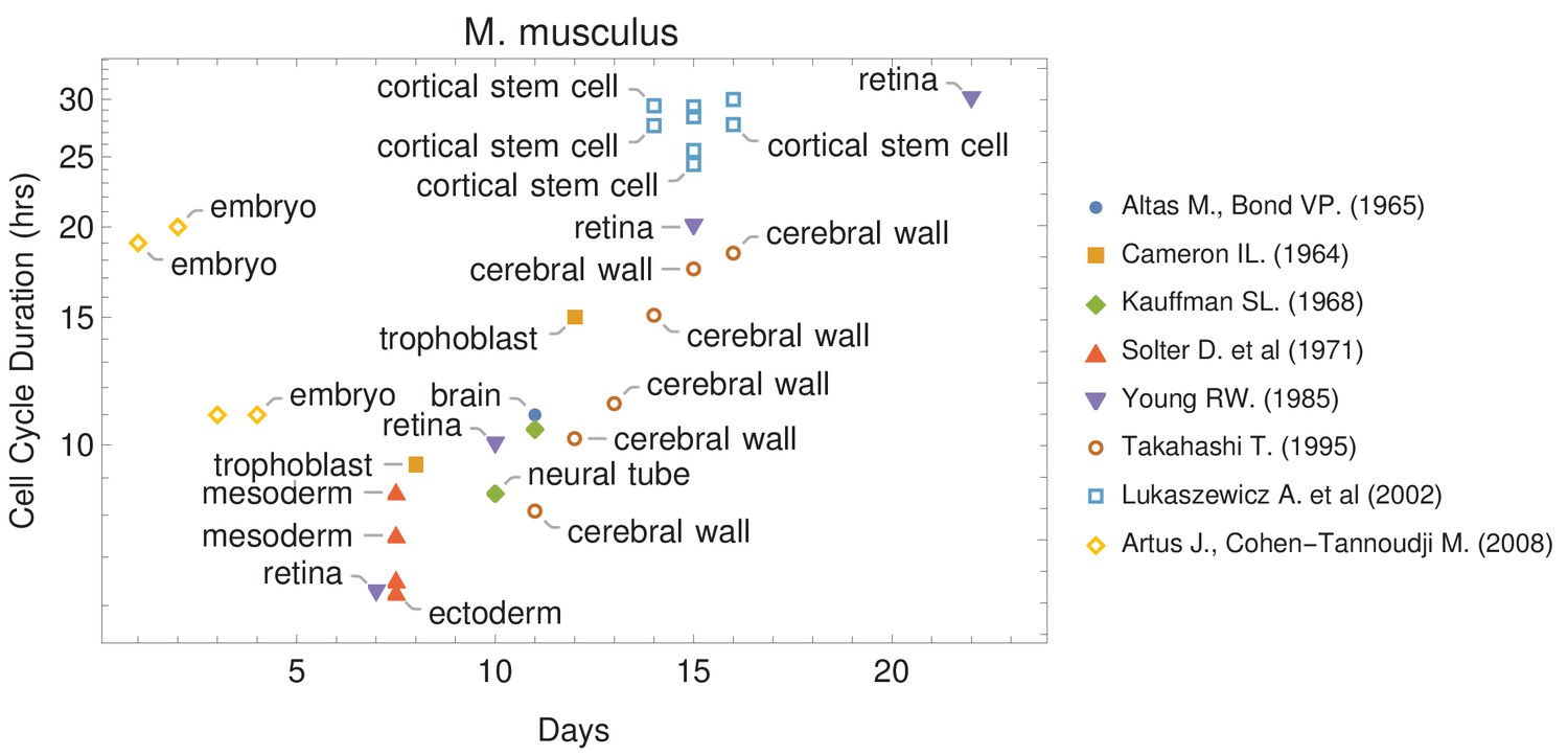
Cell cycle duration changes during mouse development.
The data was curated from several publications (PubMed identifiers: 5859018, 14105210, 5760443, 5542640, 4041905, 7666188, 12151540, 18164540), shown in the legend as authors and (year). For other species and tissues, see Supplementary file 1.
Figure 2
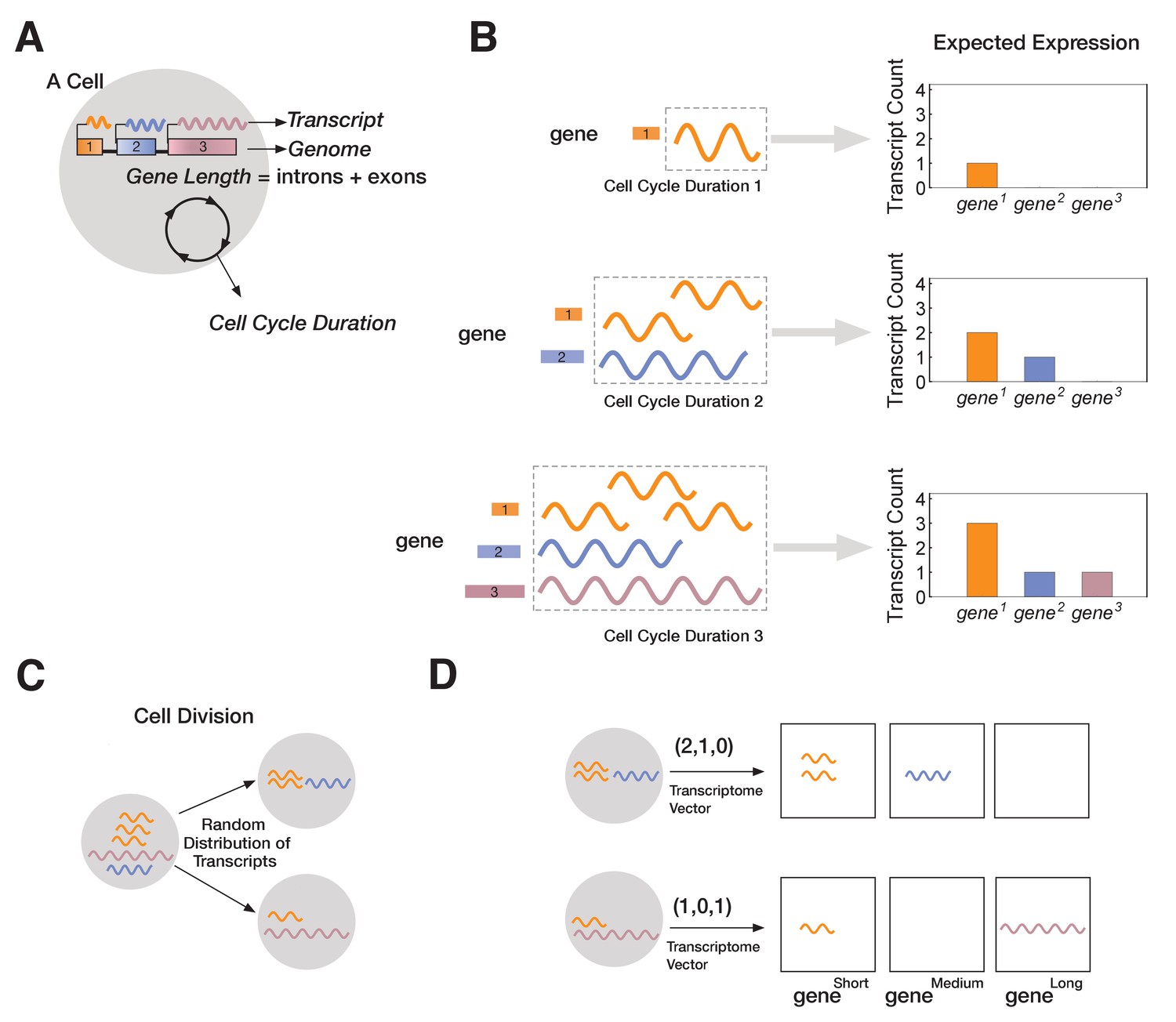
A novel mathematical model of cell lineage generation.
(A) A single cell is defined by a given number of genes in its genome as well as their gene lengths (e.g., three genes, gene1 < gene2 < gene3). Cell cycle duration defines the time a cell has available to transcribe a gene. (B) For example, a cell with cell cycle duration = 1 hr will only enable transcription of gene1; cell cycle duration = 2 hr will enable transcription of gene1 and gene2; cell cycle duration = 3 hr enables transcription of all three genes. (C) Our model assumes that transcripts passed from parental cell to its progeny will be randomly distributed during division (M-phase). (D) Each cell is characterized by its transcriptome, represented as a vector.
Figure 3 with 4 supplements
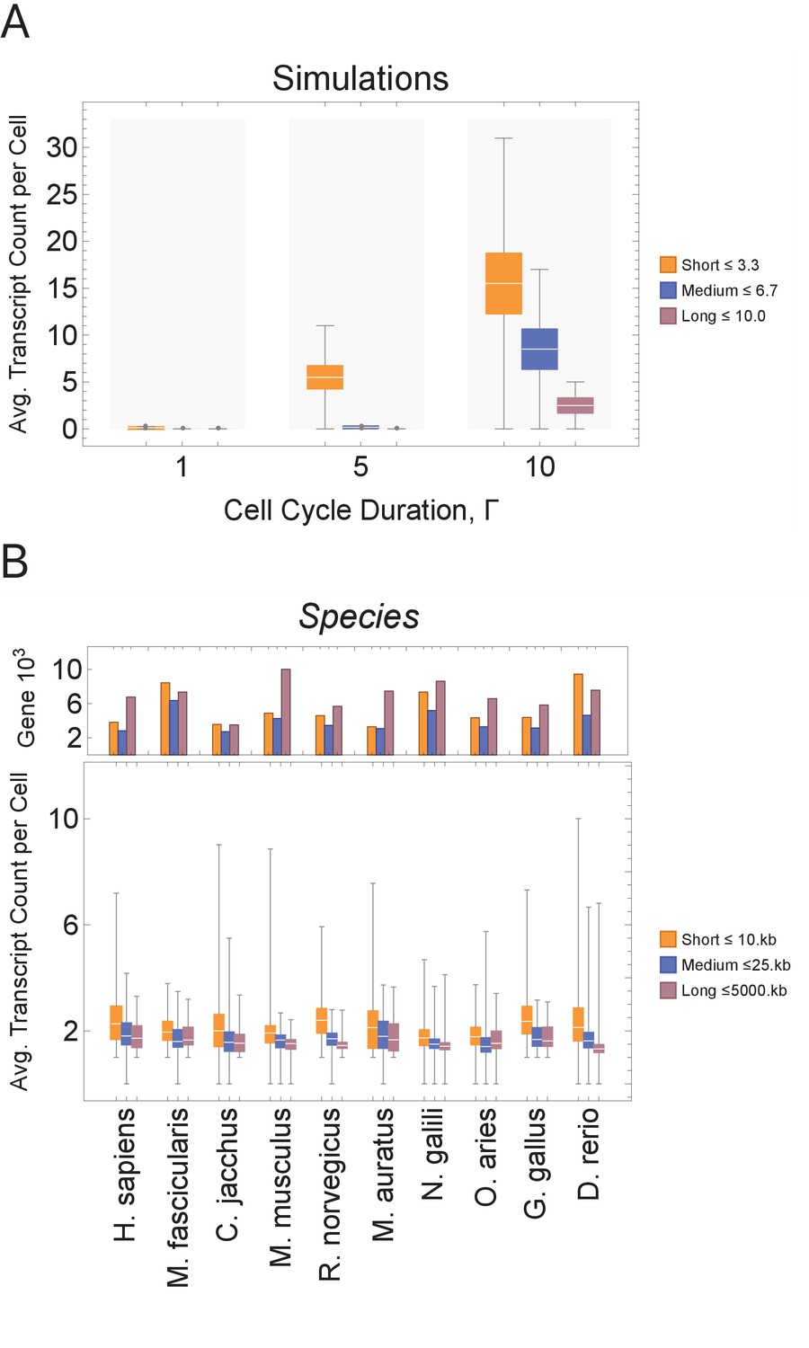
Short genes produce more transcripts than longer genes at multiple cell cycle duration lengths.
The transcriptome for each cell is subdivided into short, medium, and long gene bins, and transcript counts are averaged per bin per cell. (A) Simulations predict that short gene transcripts will be more highly expressed than long gene transcripts, irrespective of the genome size. Simulation results are shown for cell cycle durations of 1, 5, and 10 hr and gene lengths (geneL1-L10); see Figure 3—figure supplement 3 for additional simulations (other parameters ploidy = 1, one cell division, iterations = 5,000,000, genome G = 10, geneL1-L10, transcription rate, λ = 1 kb/hr, RNA polymerase II re-initiation, ). Bins are defined such that genes are evenly distributed across them. (B) Single-cell microglia data obtained from GSE134707 (Geirsdottir et al., 2019) displaying expected patterns where short genes (lengths <10 kb) have a higher transcript expression than both medium genes (lengths > 10 kb) and longer genes (lengths >25 kb) – Kolmogorov–Smirnov test p < 10−16, the upper bound p-value for all short-medium and short-long comparisons – across nine different species (age): Macaca fascicularis (3 years), Callithrix jacchus (7 years), Mus musculus (8–16 weeks), Rattus norvegicus (11–14 weeks), Mesocricetus auratus (8–16 weeks), Nannospalax galili (2-4 years), Ovis aries (18–20 months), Gallus gallus (24 weeks), and Danio rerio (4–5 months). The top part of the plot shows the total number of genes possible in each bin, given the gene length distribution of each genome. Bins are defined such that they are both consistent across all species and also approximately evenly filled with genes.
Figure 3—figure supplement 1

Simulations exploring the effects of cell cycle duration and RNA polymerase II (rnaPol II) for different re-initiation distances, , and transcription rates, λ.
(A) We conducted simulations for different re-initiation distances (default assumes that re-initiation only occurs once rnaPol II reaches the end of the gene). (B) We conducted simulations for different transcription rate. Rates were randomized using a Gaussian distribution (mean = λ, standard deviation = λ) such that transcription time T = Γλ/L. We generally assumed a fixed rate λ = 1, where all genes exhibit the same rate. Changing parameters in (A) and (B) does not alter the overall trend we observe, that short genes produce more transcripts than longer genes. Other parameters for panels (A) and (B) were ploidy = 1, Li = {1,2,3,4,5,6,7,8,9} and G = 9, one cell division, iterations = 1000. We also show in the case where all genes are the same length, L = 9, and cell cycle duration is constant (C, D) that when cell cycle durations are short, Γ = 1 hr, only high transcription rates can quench the constraint of short cell cycle. (E, F) When cell cycle duration is long, Γ = 10 hr, changing transcription parameters can directly affect transcript number. Other parameters for panels (C–F) were ploidy = 1, Li = {9}, G = 9, genome = {gene19, gene29 …, gene99}, one cell division, iterations = 1000 per panel.
Figure 3—figure supplement 2

Effects of maternal transcript inheritance.
(A) Simulation of expected transcript count when cells are initiated without maternal transcripts in comparison to cells with maternal transcripts. Parameters: gene lengths (geneL1-L10), ploidy = 1, one cell division, 10 hr cell cycle duration, iterations = 10,000. (B) Simulation of expected transcript count where a proportion (zero or half) of inherited parental transcripts remain after each cell division. Parameters: gene lengths (geneL1-L10), ploidy = 1, two cell divisions, 10 hr cell cycle duration, iterations = 1000.
Figure 3—figure supplement 3
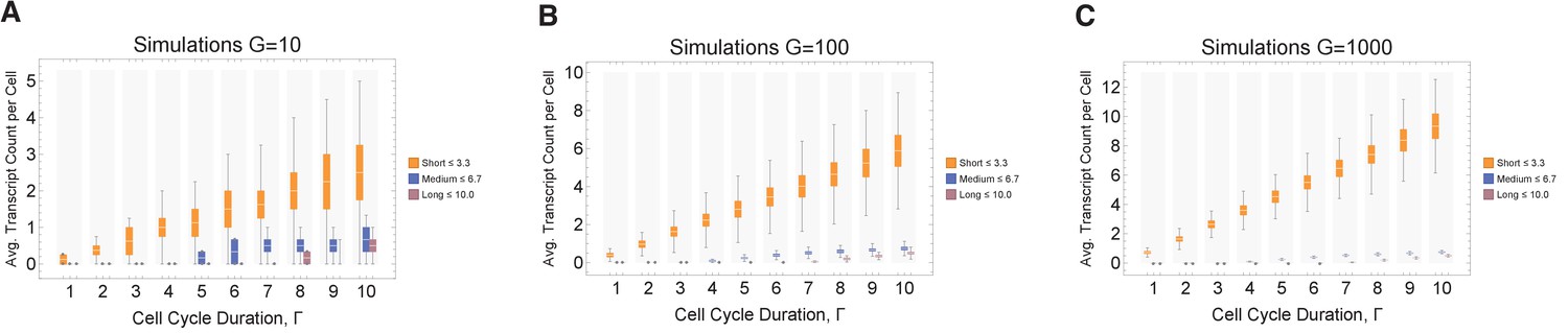
Simulations exploring the effects of cell cycle duration on transcript count per cell.
We find that short genes produce more transcripts than longer genes. We conducted simulations for different gene numbers (10, 100, and 1000; panels A, B, and C, respectively) and distributions across various cell cycle durations (1–10 hr), always resulting in the same overall trend being observed. The transcriptome for each cell is subdivided into short, medium, and long gene bins. Transcript counts in each bin are averaged for each cell. Prediction from simulation shows that cells will have higher expression of short gene transcripts and longer genes irrespective of the number of genes in each bin. However, simulation shows that longer cycle durations will increase relative transcript count per cell (other parameters ploidy = 1, one cell division, iterations = 1000, RNA polymerase II re-initiation, occurs at the end of the gene).
Figure 3—figure supplement 4
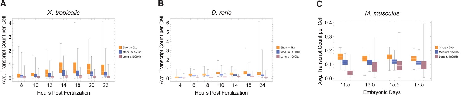
Single-cell data exploring the effects of cell cycle duration on transcript count per cell.
We find that short genes produce more transcripts than longer genes. (A) Xenopus tropicalis (Xenopus) single-cell data obtained from GSE113074 (Lib2), (B) Danio rerio (zebrafish) single-cell data obtained from GSE112294, and (C) Mus musculus (mouse) cortex single-cell data obtained from GSE107122, displaying predicted patterns where short genes have a higher average transcript expression than longer genes.
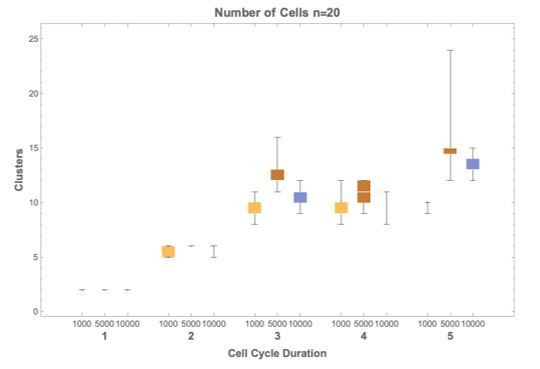
Figure 4
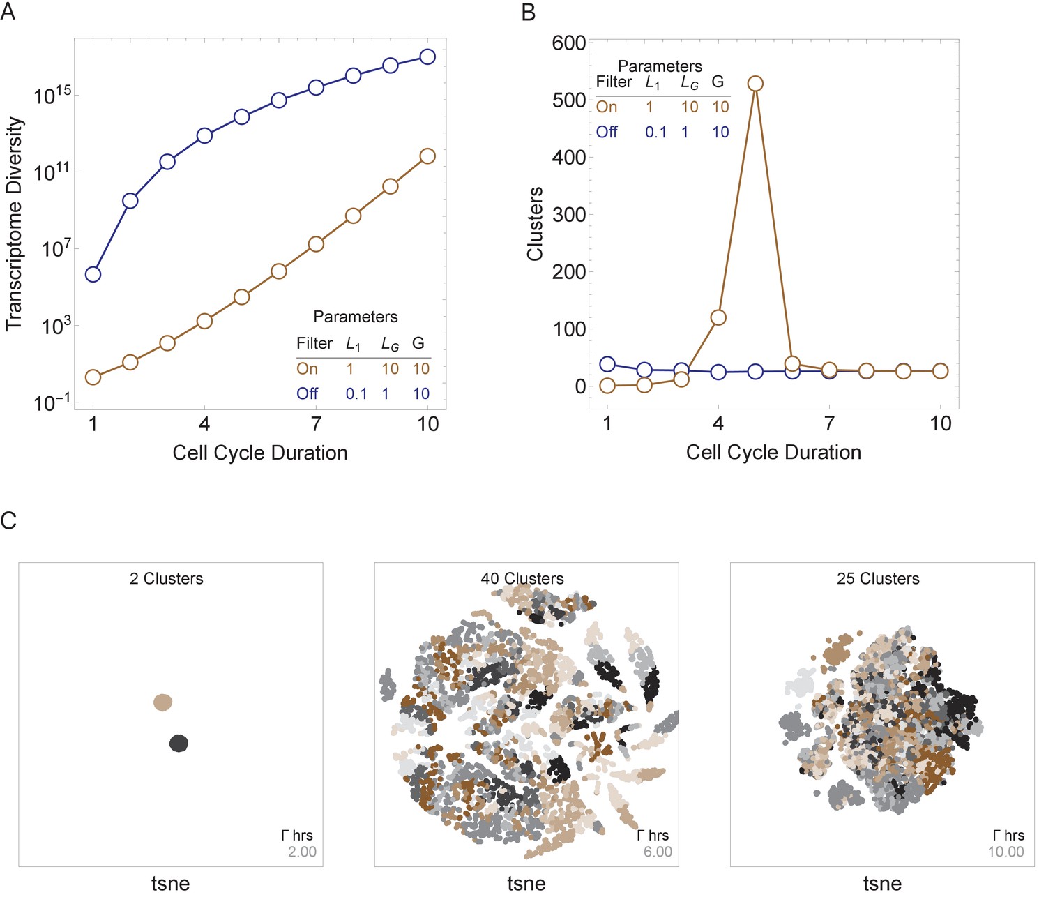
Cell cycle duration can control cell diversity.
Simulations explore the effects of cell cycle duration, Γ, gene number, G, and gene length distribution. (A) Simulations show that cell diversity (transcriptome diversity) increases as a function of cell cycle duration. Short cell cycle durations can constrain the effects of gene number as long as a transcriptional filter is active (gene length distributions are broad, ). When , cell cycle duration does not control cell diversity. Cell cycle duration effects are relative to the gene length distribution in the genome. (B) We use Seurat to cluster the simulated single-cell transcriptomes (10,000 cells) using default parameters and report the number of cell clusters over the simulations. This shows that cell diversity increases with gene number, but the number of clusters identified decreases when all the gene transcripts can be expressed similarly among all cells. (C) Representative examples (10,000 cells) of t-SNE visualizations (RunTSNE using Seurat version 3.1.2) are shown for simulations with cell cycle durations 2, 6, and 10 hr (genome G = 10, geneL1-L10, ploidy n = 1, and transcription rate, λ = 1 kb/hr, RNA polymerase II re-initiation, ).
Figure 5
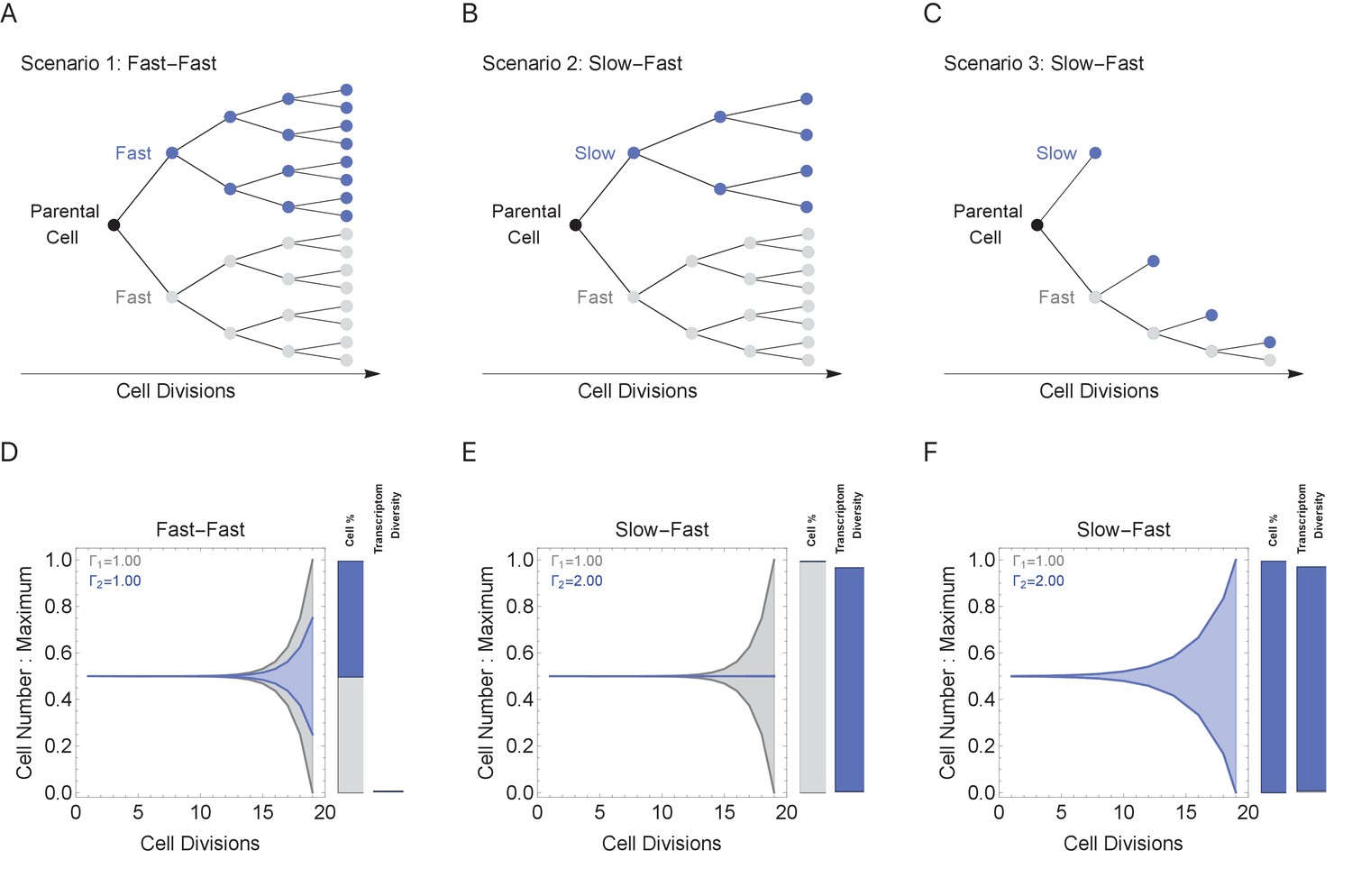
Cell cycle duration can control the generation of cell proportions and cell types within a population.
Simulations start with two cells and run for 18 divisions (generating 219 cells when cell cycles are the same). Cell1 is initialized with cell cycle duration Γ1 = 1 hr, Cell2 has cell cycle duration, Γ2, ranging from 1 to 2 hr. All progeny are tracked based on their cell cycle duration (lineage Γ1 = 1 cell cycle duration, gray, or lineage Γ2 cell cycle duration, blue). Tree plot depicting lineages when the cell cycle duration (A) is the same, Γ1 = Γ2 (scenario 1), or (B, C) differs, Γ1 < Γ2 (scenarios 2 and 3). Scenario 2 captures a situation when the cell cycle is determined by the parental lineage, while scenario 3 captures a situation when a cell splits asymmetrically into a fast and slow cell, resulting with the fast lineage having just one cell. (D–F) Müller visualizations show that when the cell cycle duration is the same, both cells contribute the same number of progeny and cell proportions (%) are 50:50 (bottom left panel). The visualization is stacked, down-scaling the blue lineage slightly to reduce occlusion of the gray lineage. Cells with longer cell cycle duration (blue lineage) generate fewer progeny with respect to the cells with a short cell cycle duration of 1 hr (gray lineage). However, the slower cells contribute more to the diversity observed in the population, shown as the blue and gray transcriptome diversity bars. Thus, increasing cell cycle duration increases cell diversity, but also limits the number of progeny generated. The system can overcome the limit on cell number by using scenario 3, where more slow cells can be generated (other parameters G = 5, gene lengths (geneL1-L2), genome = {1,1.25,1.5,1.75,2} and ploidy = 1, RNA polymerase II re-initiation, ).
Figure 6 with 2 supplements
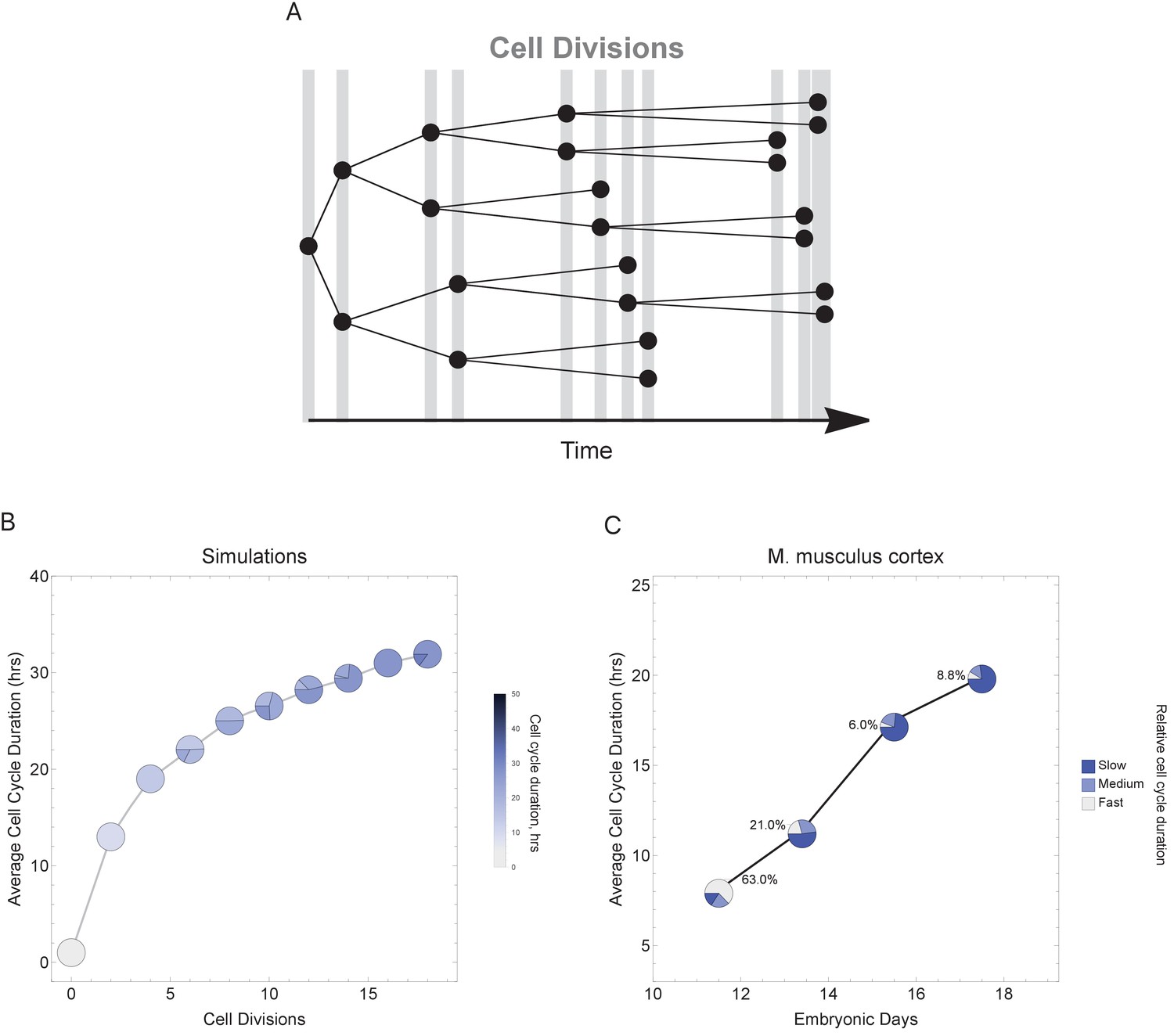
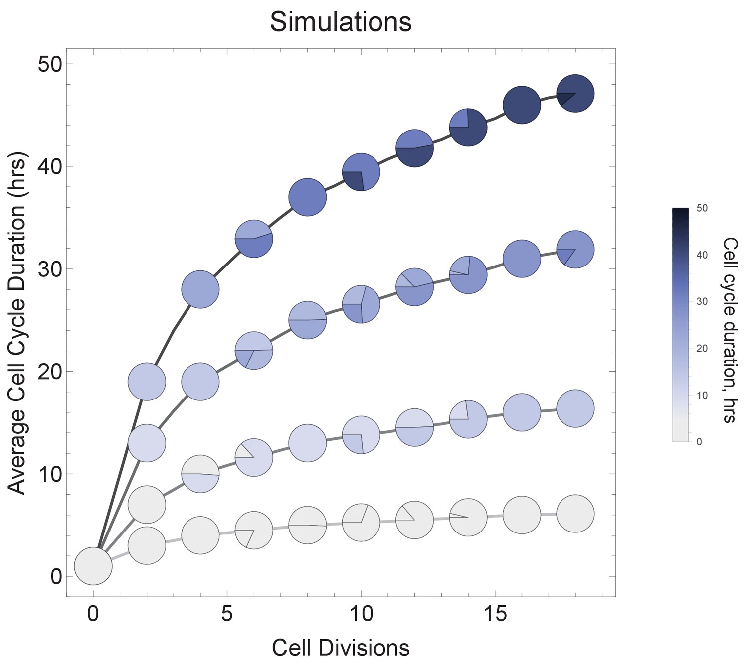
Varying cell cycle duration across time affects cell-type proportions.
(A) Cell cycle duration increases after each cell division, with amount of increase defined using a Gaussian distribution. (B) Simulation of gradually increasing cell cycle duration over time, such that Γ = Gaussian (mean Γparent ± 6, standard deviation σ = 0.06), affects the relative proportion of cells with different cell cycle durations (pie charts). All cell progeny are labeled based on their cell cycle duration (inherited from parent). See Figure 6—figure supplement 1 for results using other increment rates. Parameters: genome = 10, gene lengths (geneL1-L10), λ = 1 kb/hr, 18 cell divisions, iterations = 500, ploidy n = 1, RNA polymerase II re-initiation, . (C) Single-cell transcriptomics data from GSE107122 (Yuzwa et al., 2017) for embryonic mouse cortex development, known to exhibit increasing cell cycle duration over time. This data includes identified cell types, is a time series, and we know the average cell cycle duration at each time point; at E11.5, the average cell cycle duration is 8 hr and by E17.5 it is 18 hr (Furutachi et al., 2015; Takahashi et al., 1995a). Cells were defined as relatively fast cycling cells (apical progenitors), relatively medium cycling (intermediate progenitors), and relatively slow cycling (neurons), with cell-type annotation based on cell clustering analyses conducted in (Yuzwa et al., 2017). We show how cell proportions (pie charts) change across time, with apical progenitors (relatively fast cycling cells) decreasing in frequency as the average cell cycle duration increases.
Figure 6—figure supplement 1
Varying cell cycle duration across time affects cell-type proportions.
All cell progeny are labeled based on their cell cycle duration (inherited from parent). Each line represents a different rate of increase in average cell cycle duration, following rate increments 0 (shallowest constant curve), 1, 3, 6, and 9 (steepest curve). Cell cycle duration increases after each division using a Gaussian distribution, such that Γ = Gaussian (mean Γ parent ± rate increment, standard deviation σ = 0.06). Gradual cell cycle duration changes affect the relative proportion of cells with different cell cycle durations (pie charts). Parameters genome = 10, gene lengths (geneL1-L10), λ = 1 kb/hr, 15 cell divisions, iterations = 500, ploidy n=1, RNA polymerase II re-initiation, .
Figure 6—figure supplement 2
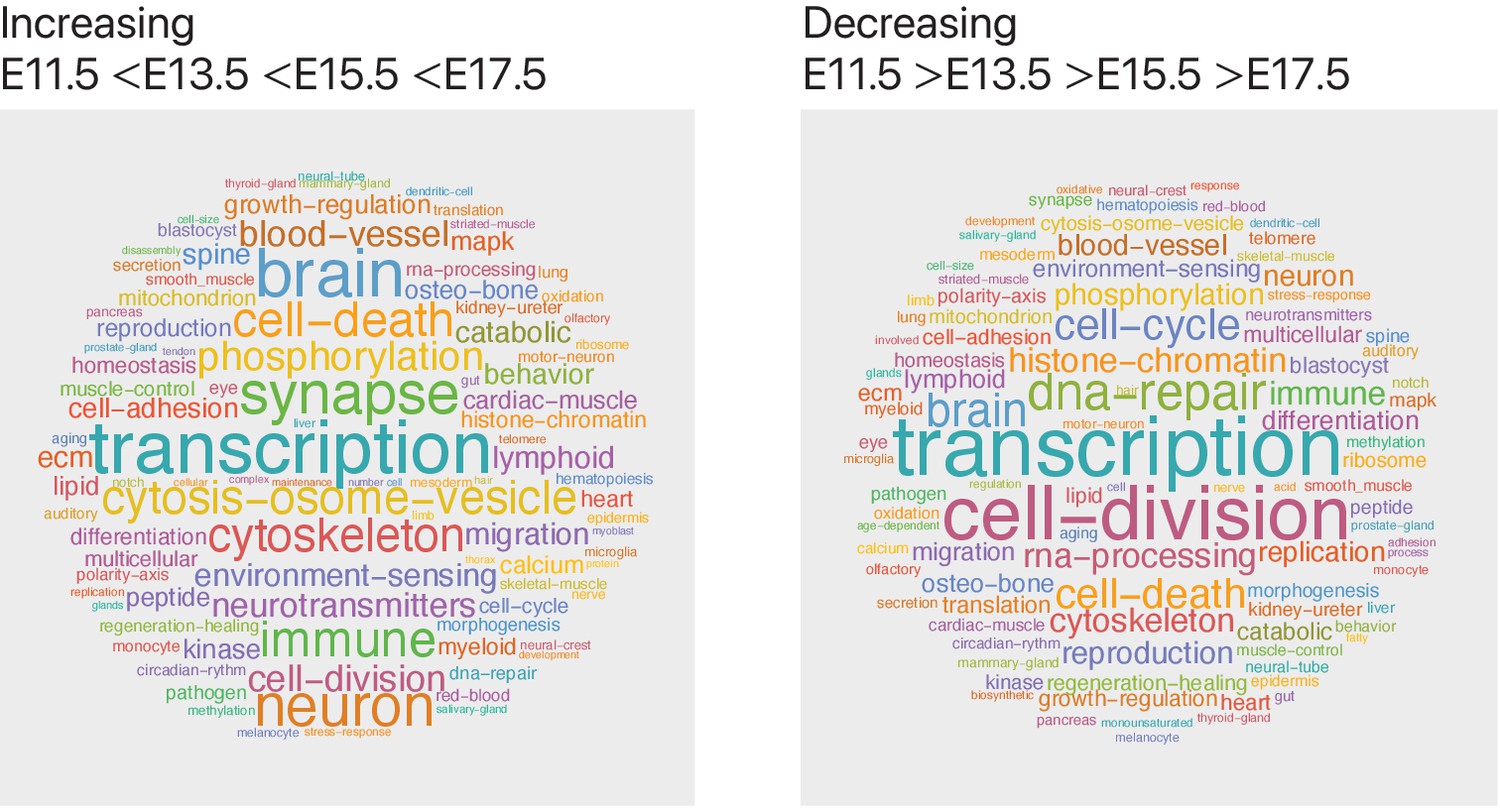
Genes with increasing transcript expression are associated with neuronal and synaptic pathways.
We used the mouse cortex time-series single-cell transcriptomics data, obtained from GSE107122 (Yuzwa et al., 2017), to identify gene transcripts that increase or decrease in expression level over development (with gene transcript expression following the pattern: E11.5 < E13.5 < E15.5 < E17.5 for increasing and E11.5 > E13.5 > E15.5 > E17.5 for decreasing genes). To summarize pathway annotation information for each gene, we identified all corresponding Gene Ontology biological process terms for each gene from the Ensembl genome database and visualized term frequencies as word clouds using Mathematica. We find that the genes (n = 2186) that increase across time are associated with neural developmental (brain, neuron, and synapse) pathways, whereas the genes (n = 1834) that decrease across time are associated with DNA-repair and proliferation pathways.
Figure 7 with 1 supplement

Gene length distribution and developmental time are correlated.
(A) Model organisms exhibit a large diversity in gene length distributions over their genomes. Species that have narrower gene length distributions tend to develop faster, while slow developers (mammals) exhibit broad and right-shifted gene length distributions. Demarcating a 1 hr cell cycle duration using an average transcription rate of 1.5 kb/min illustrates the proportion of genes that would be interrupted before transcript completion for each organism. Saccharomyces cerevisiae (budding yeast), Caenorhabditis elegans (worm), Drosophila melanogaster (fruit fly), Oikopleura dioica (tunicate), Danio rerio (zebrafish), Takifugu rubripes (fugu), Xenopus tropicalis (frog), Gallus gallus (chicken), Mus musculus (mouse), Sus scrofa (pig), Macaca mulatta (monkey), and Homo sapiens (human). (B) There is a clear positive correlation between developmental time and median gene length (101 species, Figure 7—figure supplement 1). Estimated developmental time was curated from the Encyclopedia of Life or articles found in PubMed (Supplementary file 3). We used gestation time for mammals and hatching time for species who lay eggs (since it is difficult to accurately define a comparative stage for all species). We analyzed the data using a Pearson correlation test, shown as r. For each species, we calculated median gene length: all protein coding genes were downloaded from Ensembl version 95 (Yates et al., 2016) using the R Biomart package (Durinck et al., 2009; Durinck et al., 2005). The length of each gene was calculated using start_position and end_position for each gene as extracted from Ensembl data.
Figure 7—figure supplement 1

Illustration of the association between developmental time and median gene length across 101 species, grouped by taxonomy class (Supplementary file 3).
(A) The association between number of cell types and species appearance in the fossil record according to Valentine et al., 1994. (B) The association between median gene length and emergence time. (C) The association between median gene length and developmental time across 12 species taxonomy classes (Saccharomycetes, Chromadorea, Ascidiacea, Insecta, Hyperoartia, Amphibia, Actinopterugii, Aves, Reptilia, Mammalia, Sarcopterygii, and Myxini). For each species, we calculated median gene length: the length of each gene was calculated using start and end positions for each gene as extracted from the Ensembl genome database (version 95). Estimated developmental time was curated from the Encyclopedia of Life or articles found in PubMed (Supplementary file 3). We used gestation time for mammals and hatching time for species who lay eggs (since it is difficult to accurately define a comparative stage for all species). We analyzed the data using a Pearson correlation test shown as r.
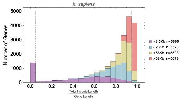
Figure 8 with 4 supplements
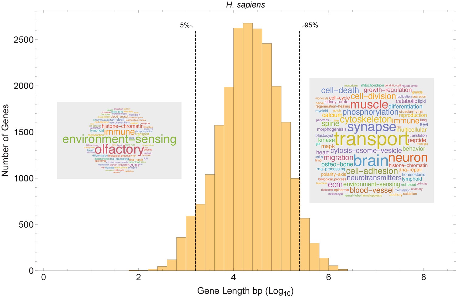
Short genes and long genes participate in different pathways.
The plot shows the H. sapiens gene length distribution. We selected the shortest 5% quantile as a list of short genes and the 95% quantile as a list of long genes. Short genes < 1.6 kb (n=1124) are involved in immune defense, environment-sensing, and olfactory, and long genes >243 kb (n = 1125) are represented in processes involving muscle and brain development, as well as morphogenesis. For each gene group, we identified all corresponding Gene Ontology (Ashburner et al., 2000) biological process terms downloaded from the Ensembl genome database version 100 (Yates et al., 2016), grouped the terms into themes (Supplementary files 5 and 6), and visualized the resulting term frequencies as word clouds using Mathematica. Refer to Figure 8—figure supplements 2 and 3 for a more detailed analysis of the themes across all gene groups.
Figure 8—figure supplement 1
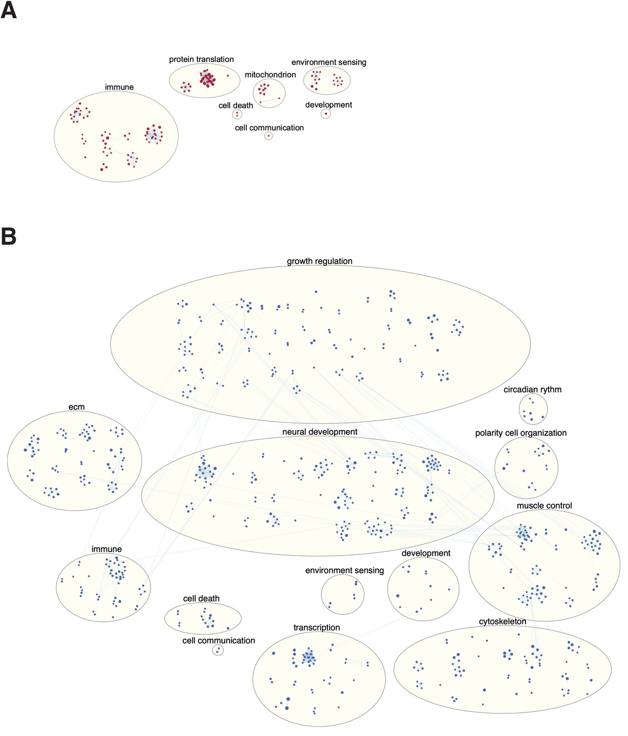
Enriched pathways in short (A) and long (B) genes in human.
Enrichment map (Merico et al., 2010) showing the pathways enriched in short genes compared to long gene. Circles represent pathway gene sets. Lines connecting circles represent overlap between pathways. Similar pathways are grouped in larger bubbles and manually labeled using the AutoAnnotate (Kucera et al., 2016), Cytoscape app (Reimand et al., 2019), and custom scripts (Supplementary file 4). Blue pathways (nodes) are enriched in long genes, and red pathways are enriched in short genes (p-value<0.05, FDR < 0.01, Jaccard coefficient > 0.25). Long genes were enriched in many more functional groups than short genes with 798 and 152 enriched pathways, respectively.
Figure 8—figure supplement 2
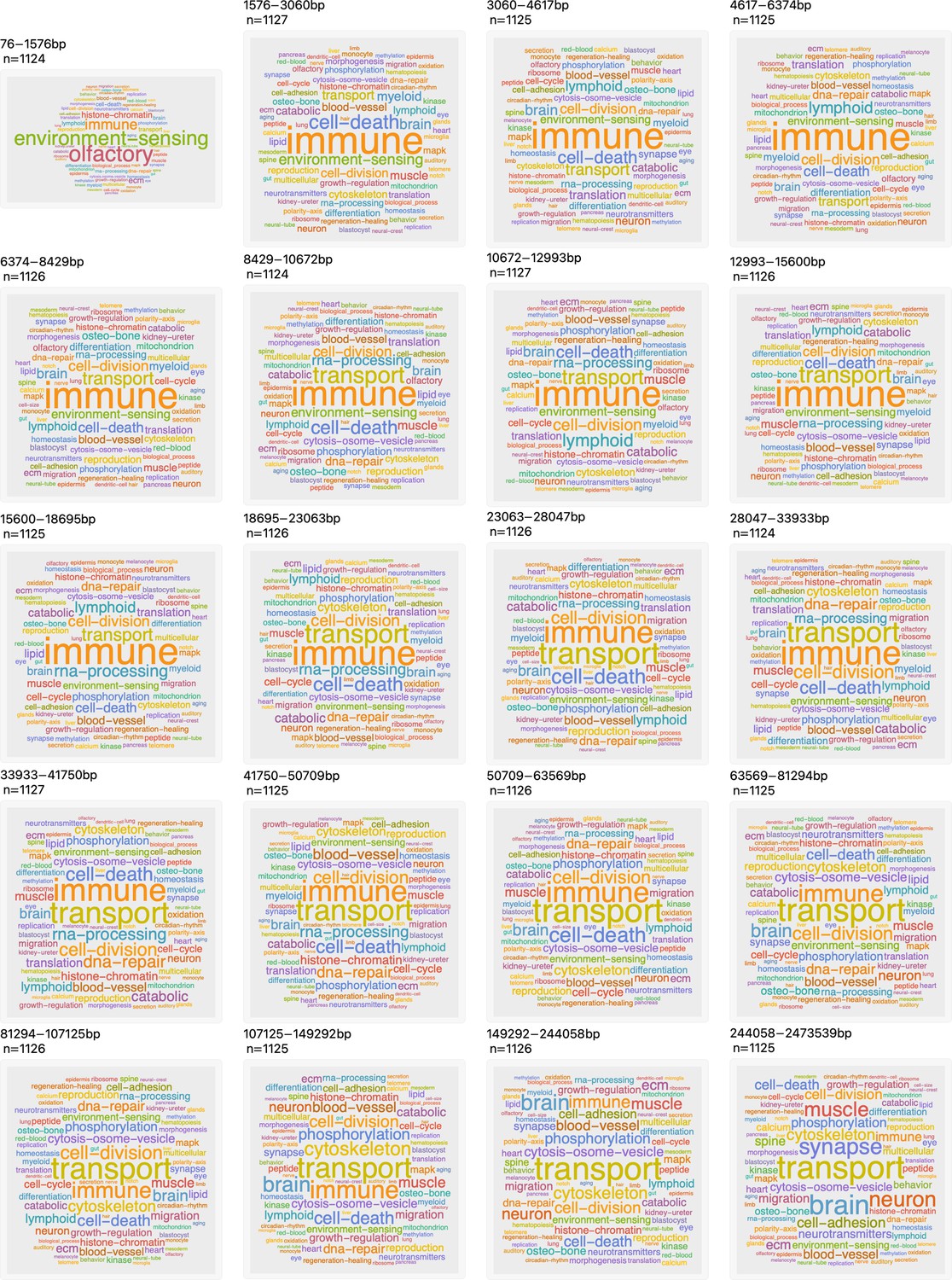
Genes participate in different pathways.
The plot shows the H. sapiens genes divided into 20 groups from shortest genes to the longest genes. For each gene group, we identified all corresponding Gene Ontology (Ashburner et al., 2000) biological process terms downloaded from the Ensembl genome database version 100 (Yates et al., 2016), grouped the terms into themes (Supplementary files 5 and 6), and visualized the resulting term frequencies as word clouds using Mathematica.
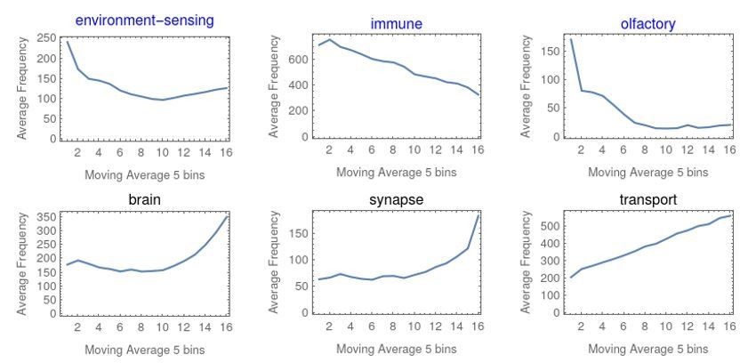
Figure 8—figure supplement 3
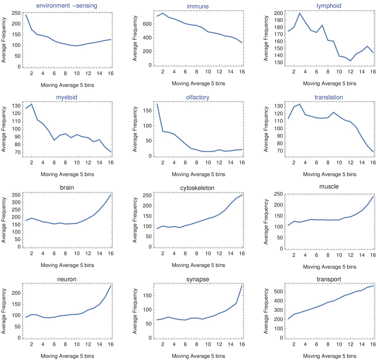
Moving average across gene length.
H. sapiens genes were divided into 20 groups from shortest genes to longest genes. For each gene group, we identified all corresponding Gene Ontology (Ashburner et al., 2000) biological process terms downloaded from the Ensembl genome database version 100 (Yates et al., 2016) and grouped the terms into themes (Supplementary files 5 and 6). We calculated a moving average to explore the trend across gene groups by theme. For example, we identified the 15 most frequent themes between the shortest (blue) and longest (black) gene groups. We found that themes such as ‘environment-sensing,’ ‘immune,’ and ‘olfactory’ show a trend with a decreasing average and are found only in the shortest gene group (blue). On the other hand, themes such as ‘brain,’ ‘muscle,’ ‘neuron,’ and ‘synapse’ show an increasing trend and are found only in the longest genes group (black).
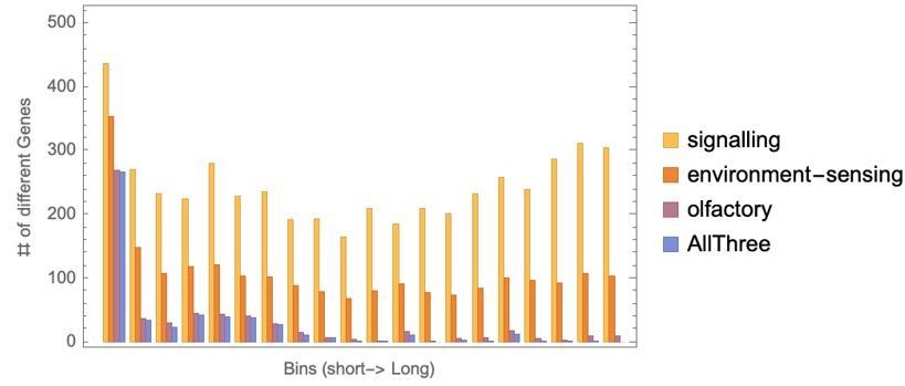
Figure 8—figure supplement 4
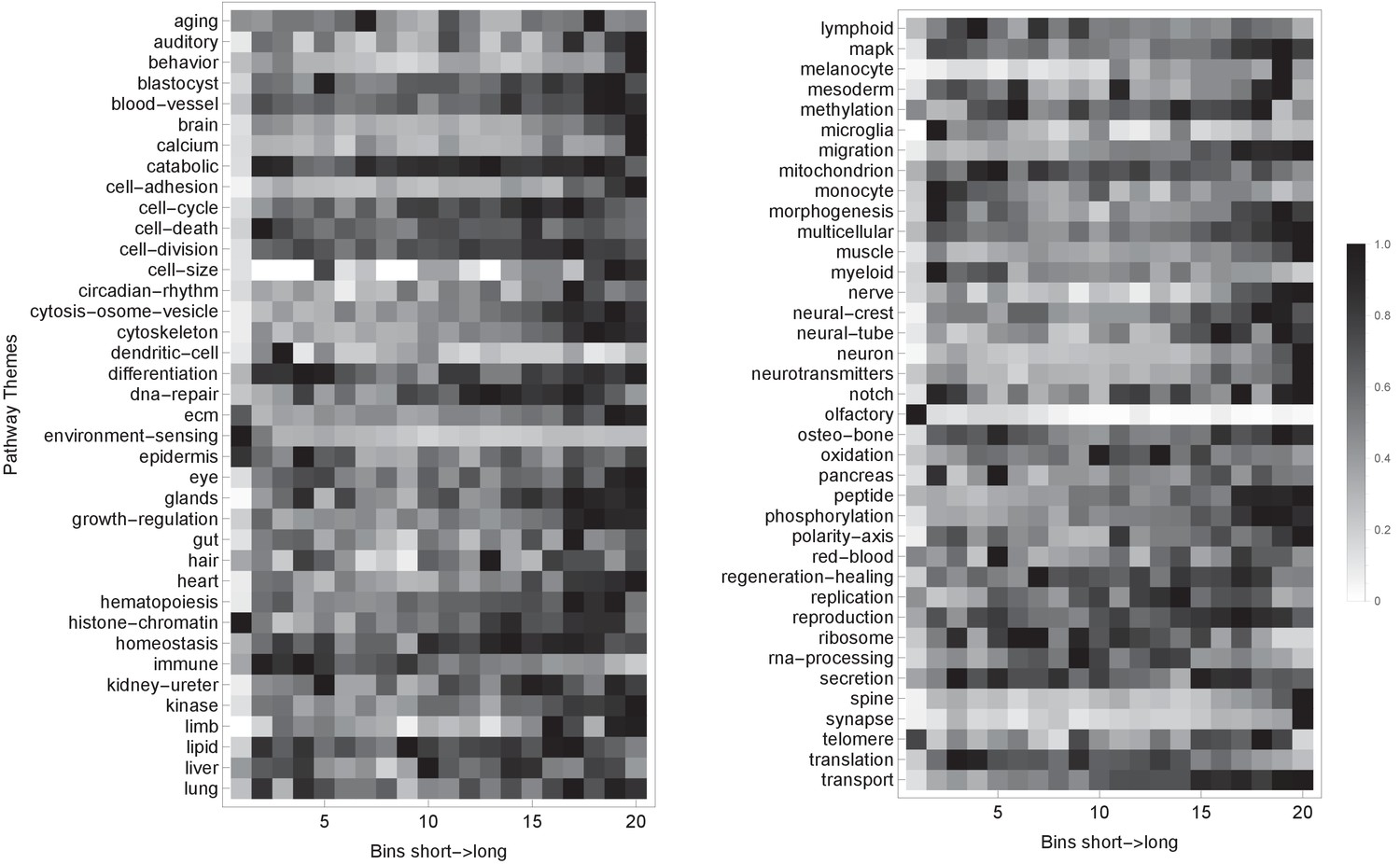
Pathway themes are associated with gene length.
The plot shows the H. sapiens genes divided into 20 groups from shortest genes to the longest genes. For each gene group, we identified all corresponding Gene Ontology (Ashburner et al., 2000) biological process terms downloaded from the Ensembl genome database version 100 (Yates et al., 2016), grouped the terms into themes (Supplementary files 5 and 6), and visualized the resulting term relative frequencies in a matrix plot using Mathematica. Darker shading indicates higher term frequency.
Figure 9
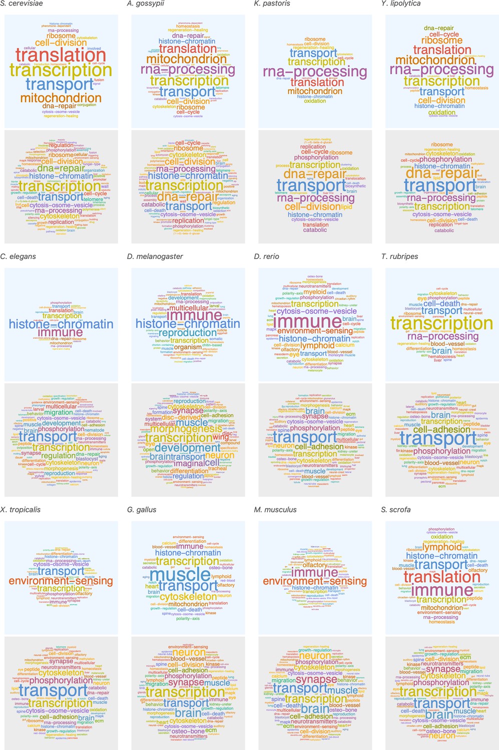
Short genes exhibit different pathways than long genes, and this trend is consistent across a wide species range.
We selected the shortest 5% quantile as a list of short genes (top panels in blue) and genes above the 95% quantile to define a list of long genes (bottom panels in gray). Saccharomyces cerevisiae (short < 0.24 kb, long > 3.5 kb), Ashbya gossypii (short < 0.36 kb, long > 3.5 kb), Komagataella pastoris (short < 0.37 kb, long > 3.3kb), Yarrowia lipolytica (short < 0.39 kb, long > 3.5 kb), Caenorhabditis elegans (short < 0.47 kb, long > 9.6 kb), Drosophila melanogaster (short < 0.56 kb, long > 29 kb), Danio rerio (short < 1.3 kb, long > 127 kb), Takifugu rubripes (short < 0.72 kb, long > 27 kb), Xenopus tropicalis (short < 0.93 kb, long > 83 kb), Gallus gallus (short < 0.67 kb, long > 104 kb), Mus musculus (short < 1.2 kb, long > 183 kb), and Sus scrofa (short < 0.57 kb, long > 197 kb). For each gene group, we identified all corresponding Gene Ontology biological process terms from the Ensembl genome database (100) and visualized the resulting term frequencies as word clouds using Mathematica.
Figure 10
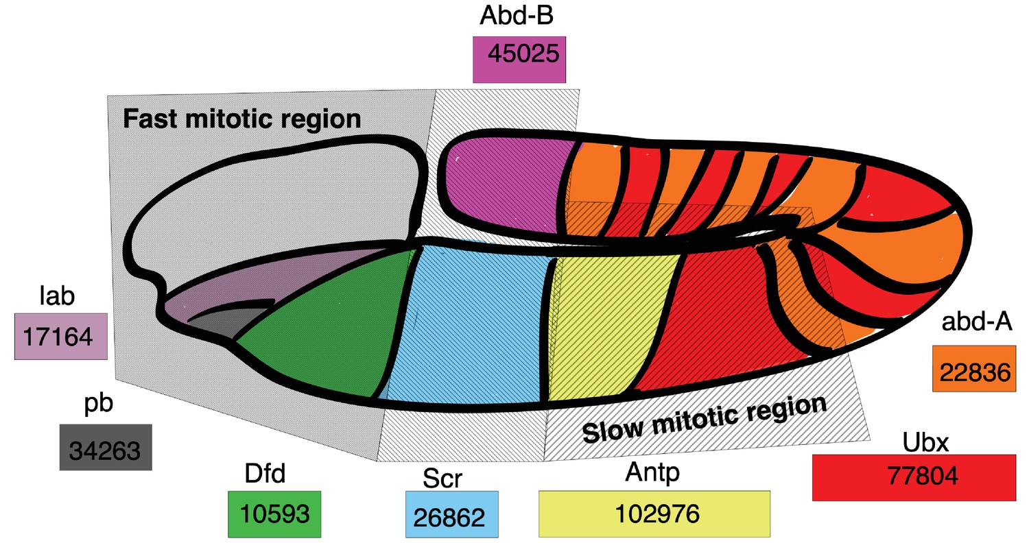
Hox gene length is correlated with spatial expression and cell cycle duration in the D. melanogaster embryo.
Drosophila Hoxd family genes are each represented by a colored rectangle, containing the length of the gene in base pairs. Spatial expression of a gene transcript is marked by its corresponding color on the Drosophila embryo map. Hoxd gene length is correlated with the cell cycle duration of the embryo location where the gene transcript is expressed, with short Hox gene transcripts expressed in regions with short mitotic cycles and long Hox gene transcripts expressed in regions of long mitotic cycles. Spatial map of cell cycle duration from Foe, 1989; Foe and Alberts, 1983 and gene transcript expression from Mallo and Alonso, 2013.
Author response image 1
Author response image 2
Author response image 3
Example gene function themes with strong trends associated with short (blue) or long (black) genes.
Author response image 4
Tables
Key resources table
| Reagent type (species) or resource | Designation | Source or reference | Identifiers | Additional information |
|---|---|---|---|---|
| Software, algorithm | Wolfram, 2017 | Mathematica (Wolfram Research Inc, Mathematica Versions 11.0–12, Champlain, IL, 2017) http://www.wolfram.com/mathematica/ | ||
| Software, algorithm | This paper | Cell developmental modelhttps://github.com/BaderLab/Cell_Cycle_Theory | ||
| Software, algorithm | PMID:25867923 Satija et al., 2015 | Seurat (3.1.2) https://satijalab.org/seurat/ | ||
| Software, algorithm | PMID:26687719 Yates et al., 2016 | Ensembl (95) and (100) https://useast.ensembl.org/index.html | ||
| Software, algorithm | PMID:10802651 Ashburner et al., 2000 | Gene Ontology http://geneontology.org/ | ||
| Software, algorithm | PMID:16082012 Durinck et al., 2005 | BioMart (3.10) http://useast.ensembl.org/biomart/martview/ | ||
| Software, algorithm | PMID:21085593 Merico et al., 2010 | Enrichment Map software (3.3.0) https://www.baderlab.org/Software/EnrichmentMap | ||
| Software, algorithm | PMID:14597658 Kucera et al., 2016 | AutoAnnotate App https://baderlab.org/Software/AutoAnnotate | ||
| Software, algorithm | PMID:14597658 Shannon et al., 2003 | Cytoscape (3.8.0) https://cytoscape.org/ | ||
| Software, algorithm | PMID:30664679 Reimand et al., 2019 | Baderlab pathway resource (updated June 1, 2020) http://download.baderlab.org/EM_Genesets/ |
Additional files
-
Supplementary file 1
Curated cell cycle duration data.
- https://cdn.elifesciences.org/articles/64951/elife-64951-supp1-v2.docx
-
Supplementary file 2
Simulations supporting transcriptome diversity analytical solution.
- https://cdn.elifesciences.org/articles/64951/elife-64951-supp2-v2.xlsx
-
Supplementary file 3
Curated developmental time for species and their corresponding median gene length.
The length of each gene was calculated using start and end positions for each gene as extracted from the Ensembl genome database (version 95). Estimated developmental time was curated from the Encyclopedia of Life or articles found in PubMed.
- https://cdn.elifesciences.org/articles/64951/elife-64951-supp3-v2.docx
-
Supplementary file 4
General pathway themes from Figure 8—figure supplement 1 generated by using a mixture of automatic classification applying key words and manual identification.
- https://cdn.elifesciences.org/articles/64951/elife-64951-supp4-v2.xlsx
-
Supplementary file 5
General pathway themes and their corresponding list of words that were used to manually classify the pathways in Figure 8 and Figure 8—figure supplements 2 and 3.
- https://cdn.elifesciences.org/articles/64951/elife-64951-supp5-v2.csv
-
Supplementary file 6
General pathway themes in Figure 8 and Figure 8—figure supplements 2 and 3 applied to H. sapiens and their corresponding Gene Ontology identifiers descriptions extracted from the Ensembl genome database.
- https://cdn.elifesciences.org/articles/64951/elife-64951-supp6-v2.csv
-
Transparent reporting form
- https://cdn.elifesciences.org/articles/64951/elife-64951-transrepform-v2.docx
Download links
A two-part list of links to download the article, or parts of the article, in various formats.
Downloads (link to download the article as PDF)
Open citations (links to open the citations from this article in various online reference manager services)
Cite this article (links to download the citations from this article in formats compatible with various reference manager tools)
Control of tissue development and cell diversity by cell cycle-dependent transcriptional filtering
eLife 10:e64951.
https://doi.org/10.7554/eLife.64951


