Likelihood approximation networks (LANs) for fast inference of simulation models in cognitive neuroscience
- Department of Cognitive, Linguistic and Psychological Sciences, Brown University, United States
- Carney Institute for Brain Science, Brown University, United States
- Psychology and Neuroscience Department, Boston College, United States
Figures
Figure 1
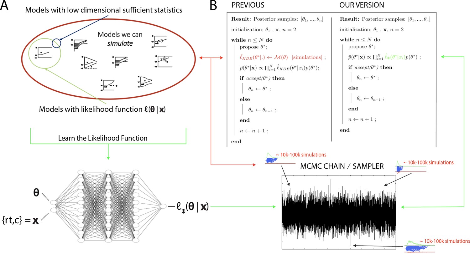
High level overview of the proposed methods.
(A) The space of theoretically interesting models in the cognitive neurosciences (red) is much larger than the space of mechanistic models with analytical likelihood functions (green). Traditional approximate Bayesian computation (ABC) methods require models that have low-dimensional sufficient statistics (blue). (B) illustrates how likelihood approximation networks can be used in lieu of online simulations for efficient posterior sampling. The left panel shows the predominant 'probability density approximation' (PDA) method used for ABC in the cognitive sciences (Turner et al., 2015). For each step along a Markov chain, 10K–100K simulations are required to obtain a single likelihood estimate. The right panel shows how we can avoid the simulation steps during inference using amortized likelihood networks that have been pretrained using empirical likelihood functions (operationally in this paper: kernel density estimates and discretized histograms).
Figure 2
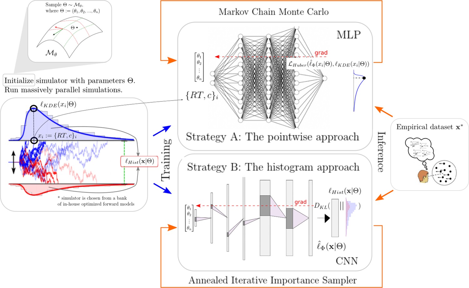
High-level overview of our approaches.
For a given model , we sample model parameters θ from a region of interest (left 1) and run 100k simulations (left 2). We use those simulations to construct a kernel density estimate-based empirical likelihood, and a discretized (histogram-like) empirical likelihood. The combination of parameters and the respective likelihoods is then used to train the likelihood networks (right 1). Once trained, we can use the multilayered perceptron and convolutional neural network for posterior inference given an empirical/experimental dataset (right 2).
Figure 3
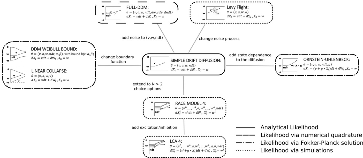
Pictorial representation of the stochastic simulators that form our test bed.
Our point of departure is the standard simple drift diffusion model (DDM) due to its analytical tractability and its prevalence as the most common sequential sampling model (SSM) in cognitive neuroscience. By systematically varying different facets of the DDM, we test our likelihood approximation networks (LANs) across a range of SSMs for parameter recovery, goodness of fit (posterior predictive checks), and inference runtime. We divide the resulting models into four classes as indicated by the legend. We consider the simple DDM in the analytical likelihood (solid line) category, although, strictly speaking, the likelihood involves an infinite sum and thus demands an approximation algorithm introduced by Navarro and Fuss, but this algorithm is sufficiently fast to evaluate so that it is not a computational bottleneck. The full-DDM needs numerical quadrature (dashed line) to integrate over variability parameters, which inflates the evaluation time by 1–2 orders of magnitude compared to the simple DDM. Similarly, likelihood approximations have been derived for a range of models using the Fokker–Planck equations (dotted-dashed line), which again incurs nonsignificant evaluation cost. Finally, for some models no approximations exist and we need to resort to computationally expensive simulations for likelihood estimates (dotted line). Amortizing computations with LANs can substantially speed up inference for all but the analytical likelihood category (but see runtime for how it can even provide speedup in that case for large datasets).
Figure 4
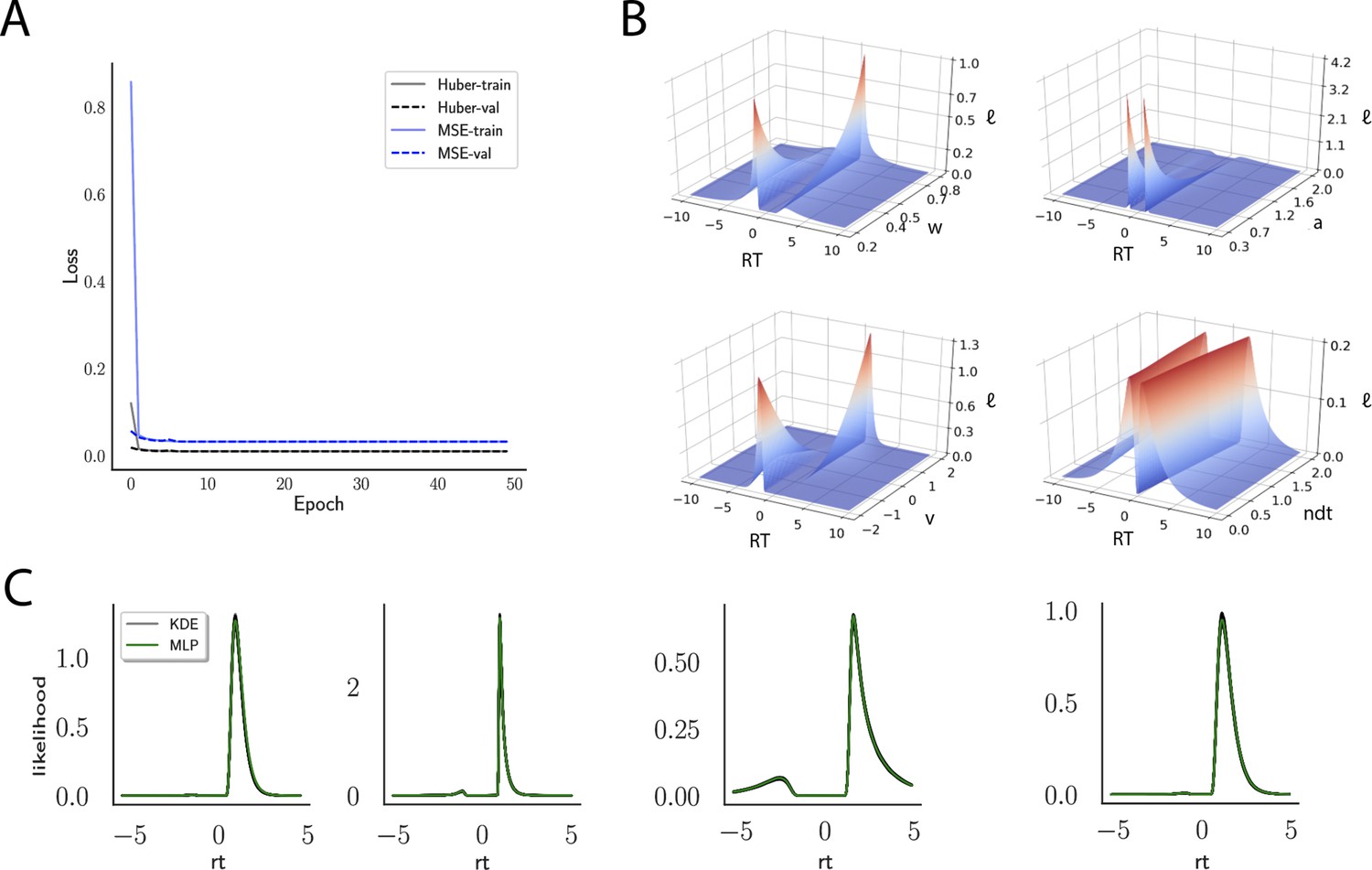
Likelihoods and manifolds: DDM.
(A) shows the training and validation loss for the multilayered perceptron (MLP) for the drift diffusion model across epochs. Training was driven by the Huber loss. The MLP learned the mapping , that is, the log-likelihood of a single-choice/RT datapoint given the parameters. Training error declines rapidly, and validation loss trailed training loss without further detriment (no overfitting). Please see Figure 2 and the 'Materials and methods' section for more details about training procedures. (B) illustrates the marginal likelihood manifolds for choices and RTs by varying one parameter in the trained region. Reaction times are mirrored for choice options −1, and 1, respectively, to aid visualization. (C) shows MLP likelihoods in green for four random parameter vectors, overlaid on top of a sample of 100 kernel density estimate (KDE)-based empirical likelihoods derived from 100k samples each. The MLP mirrors the KDE likelihoods despite not having been explicitly trained on these parameters. Moreover, the MLP likelihood sits firmly at the mean of sample of 100 KDEs. Negative and positive reaction times are to be interpreted as for (B).
Figure 5
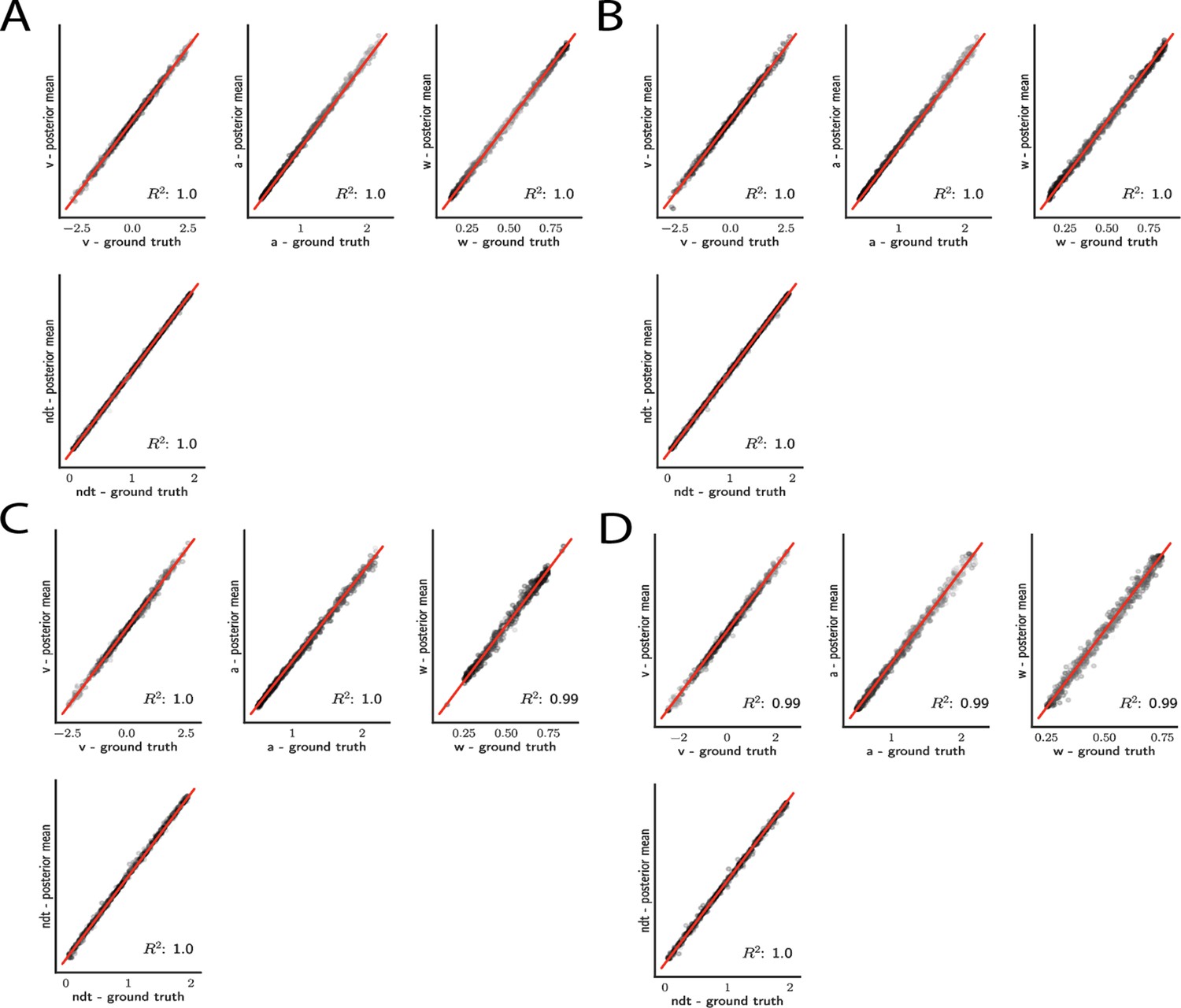
Simple drift diffusion model parameter recovery results for (A) analytical likelihood (ground truth), (B) multilayered perceptron (MLP) trained on analytical likelihood, (C) MLP trained on kernel density estimate (KDE)-based likelihoods (100K simulations per KDE), and (D) convolutional neural network trained on binned likelihoods.
The results represent posterior means, based on inference over datasets of size ‘trials’. Dot shading is based on parameter-wise normalized posterior variance, with lighter shades indicating larger posterior uncertainty of the parameter estimate.
Figure 6
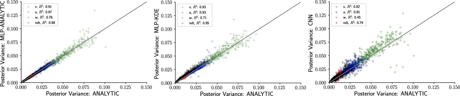
Inference using likelihood approximation networks (LANs) recovers posterior uncertainty.
Here, we leverage the analytic solution for the drift diffusion model to plot the ‘ground truth’ posterior variance on the x-axis, against the posterior variance from the LANs on the y-axis. (Left) Multilayered perceptrons (MLPs) trained on the analytical likelihood. (Middle) MLPs trained on kernel density estimate-based empirical likelihoods. (Right) Convolutional neural networks trained on binned empirical likelihoods. Datasets were equivalent across methods for each model (left to right) and involved samples.
Figure 7
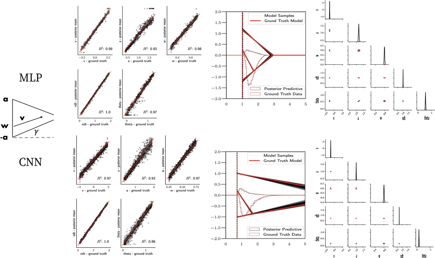
Linear collapse model parameter recovery and posterior predictives.
(Left) Parameter recovery results for the multilayered perceptron (top) and convolutional neural network (bottom). (Right) Posterior predictive plots for two representative datasets. Model samples of all parameters (black) match those from the true generative model (red), but one can see that for the lower dataset, the bound trajectory is somewhat more uncertain (more dispersion of the bound). In both cases, the posterior predictive (black histograms) is shown as predicted choice proportions and RT distributions for upper and lower boundary responses, overlaid on top of the ground truth data (red; hardly visible since overlapping/matching).
Figure 8
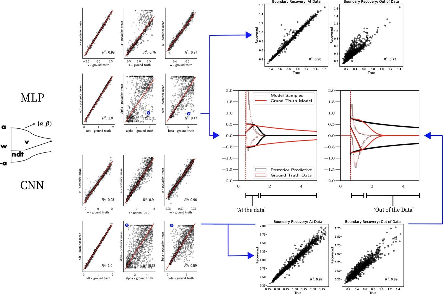
Weibull model parameter recovery and posterior predictives.
(Left) Parameter recovery results for the multilayered perceptron (top) and convolutional neural network (bottom). (Right) Posterior predictive plots for two representative datasets in which parameters were poorly estimated (denoted in blue on the left). In these examples, model samples (black) recapitulate the generative parameters (red) for the nonboundary parameters, and the recovered bound trajectory is poorly estimated relative to the ground truth, despite excellent posterior predictives in both cases (RT distributions for upper and lower boundary, same scheme as Figure 7). Nevertheless, one can see that the net decision boundary is adequately recovered within the range of the RT data that are observed. Across all datasets, the net boundary is well recovered within the range of the data observed, and somewhat less so outside of the data, despite poor recovery of individual Weibull parameters α and β.
Figure 9
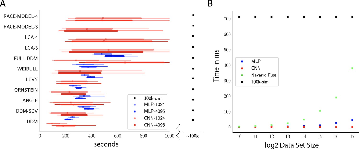
Computation times.
(A) Comparison of sampler timings for the multilayered perceptron (MLP) and convolutional neural network (CNN) methods, for datasets of size 1024 and 4096 (respectively MLP-1024, MLP-4096, CNN-1024, CNN-4096). For comparison, we include a lower bound estimate of the sample timings using traditional PDA approach during online inference (using 100k online simulations for each parameter vector). 100K simulations were used because we found this to be required for sufficiently smooth likelihood evaluations and is the number of simulations used to train our networks; fewer samples can of course be used at the cost of worse estimation, and only marginal speedup since the resulting noise in likelihood evaluations tends to prevent chain mixing; see Holmes, 2015. We arrive at 100k seconds via simple arithmetic. It took our slice samplers on average approximately 200k likelihood evaluations to arrive at 2000 samples from the posterior. Taking 500 ms * 200,000 gives the reported number. Note that this is a generous but rough estimate since the cost of data simulation varies across simulators (usually quite a bit higher than the drift diffusion model [DDM] simulator). Note further that these timings scale linearly with the number of participants and task conditions for the online method, but not for likelihood approximation networks, where they can be in principle be parallelized. (B) compares the timings for obtaining a single likelihood evaluation for a given dataset. MLP and CNN refer to Tensorflow implementations of the corresponding networks. Navarro Fuss refers to a cython (Behnel et al., 2010) (cpu) implementation of the algorithm suggested (Navarro and Fuss, 2009) for fast evaluation of the analytical likelihood of the DDM. 100k-sim refers to the time it took a highly optimized cython (cpu) version of a DDM sampler to generate 100k simulations (averaged across 100 parameter vectors).
Figure 10
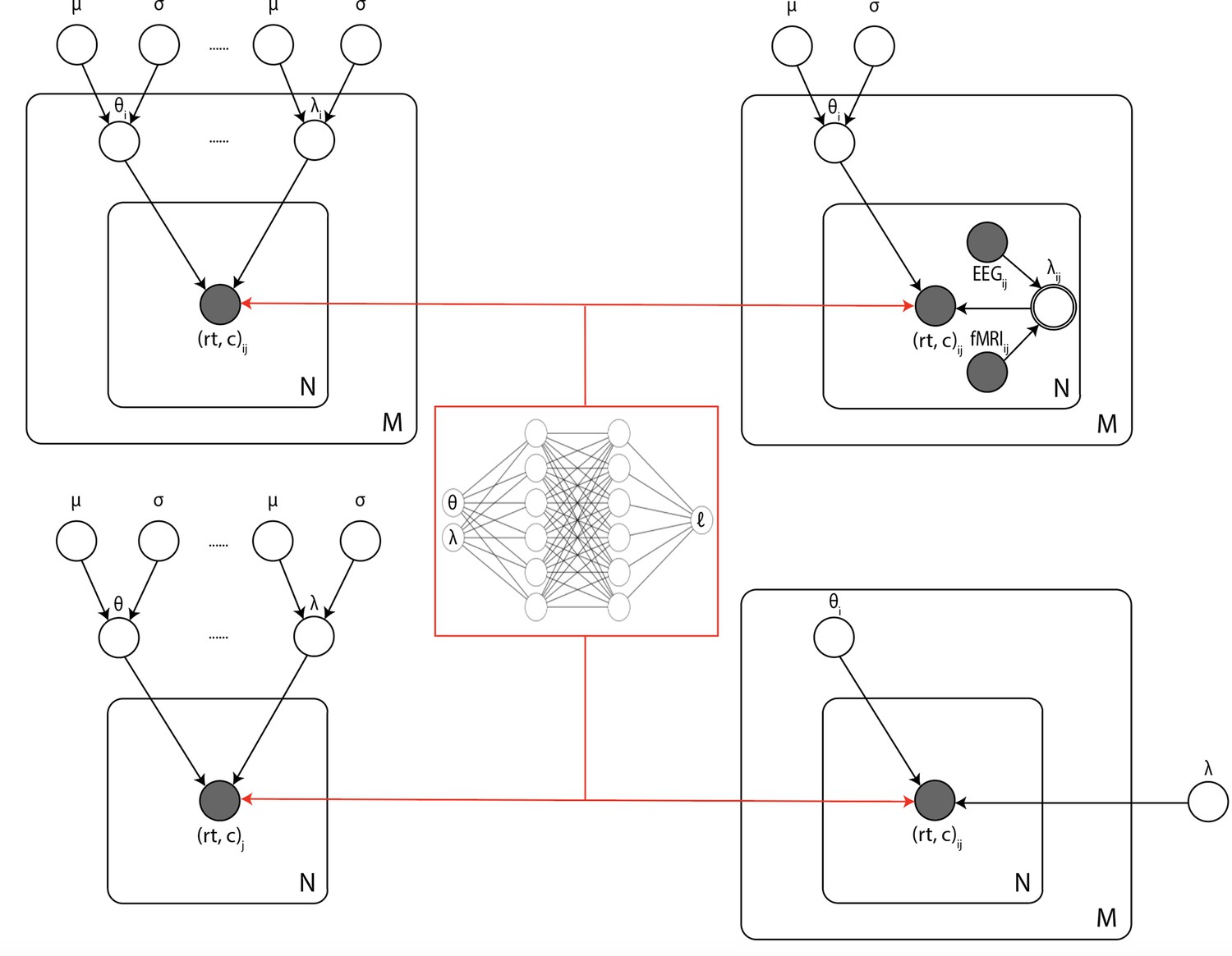
Illustration of the common inference scenarios applied in the cognitive neurosciences and enabled by our amortization methods.
The figure uses standard plate notation for probabilistic graphical models. White single circles represent random variables, white double circles represent variables computed deterministically from their inputs, and gray circles represent observations. For illustration, we split the parameter vector of our simulator model (which we call θ in the rest of the paper) into two parts θ and λ since some, but not all, parameters may sometimes vary across conditions and/or come from global distribution. (Upper left) Basic hierarchical model across M participants, with N observations (trials) per participant. Parameters for individuals are assumed to be drawn from group distributions. (Upper right) Hierarchical models that further estimate the impact of trial-wise neural regressors onto model parameters. (Lower left) Nonhierarchical, standard model estimating one set of parameters across all trials. (Lower right) Common inference scenario in which a subset of parameters (θ) are estimated to vary across conditions M, while others (λ) are global. Likelihood approximation networks can be immediately repurposed for all of these scenarios (and more) without further training.
Figure 11
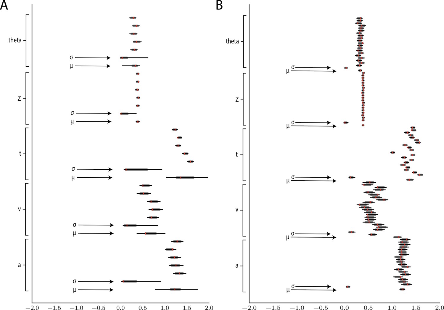
Hierarchical inference results using the multilayered perceptron likelihood imported into the HDDM package.
(A) Posterior inference for the linear collapse model on a synthetic dataset with 5 participants and 500 trials each. Posterior distributions are shown with caterpillar plots (thick lines correspond to percentiles, thin lines correspond to percentiles) grouped by parameters (ordered from above . Ground truth simulated values are denoted in red. (B) Hierarchical inference for synthetic data comprising 20 participants and 500 trials each. μ and σ indicate the group-level mean and variance parameters. Estimates of group-level posteriors improve with more participants as expected with hierarchical methods. Individual-level parameters are highly accurate for each participant in both scenarios.
Figure 12
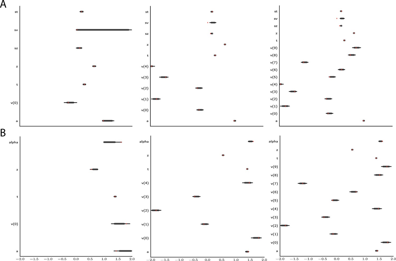
Effect of multiple experimental conditions on inference.
The panel shows an example of posterior inference for 1, (left), 5 (middle), and 10 (right) conditions. (A) and (B) refer to the full drift diffusion model (DDM) and Levy model, respectively. The drift parameter is estimated to vary across conditions, while the other parameters are treated as global across conditions. Inference tends to improve for all global parameters when adding experimental conditions. Importantly, this is particularly evident for parameters that are otherwise notoriously difficult to estimate such as (trial-by-trial variance in drift in the full-DDM) and α (the noise distribution in the Levy model). Red stripes show the ground truth values of the given parameters.
Appendix 1—figure 1
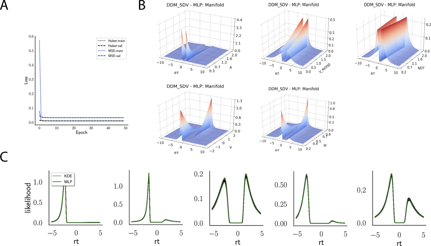
Likelihoods and manifolds: DDM-SDV.
(A) shows the training and validation loss for Huber as well as mean squared error (MSE) for the drift diffusion model (DDM)-SDV model. Training was driven by the Huber loss. (B) illustrates the likelihood manifolds by varying one parameter in the trained region. (C) shows multilayered perceptron likelihoods in green on top of a sample of 50 kernel density estimate-based empirical likelihoods derived from 20k samples each.
Appendix 1—figure 2
Likelihoods and manifolds: linear collapse.
(A) shows the training and validation loss for Huber as well as MSE for the linear collapse model. Training was driven by the Huber loss. (B) illustrates the likelihood manifolds by varying one parameter in the trained region. (C) shows multilayered perceptron likelihoods in green on top of a sample of 50 kernel density estimate-based empirical likelihoods derived from 20k samples each.
Appendix 1—figure 3
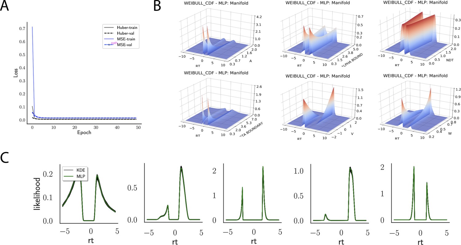
Likelihoods and manifolds: Weibull.
(A) shows the training and validation loss for Huber as well as MSE for the Weibull model. Training was driven by the Huber loss. (B) illustrates the likelihood manifolds by varying one parameter in the trained region. (C) shows multilayered perceptron likelihoods in green on top of a sample of 50 kernel density estimate-based empirical likelihoods derived from 100k samples each.
Appendix 1—figure 4
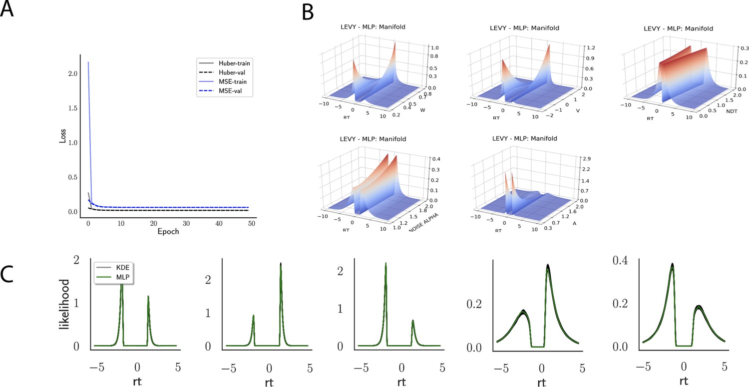
Likelihoods and Manifolds: Levy.
(A) shows the training and validation loss for Huber as well as MSE for the Levy model. Training was driven by the Huber loss. (B) illustrates the likelihood manifolds by varying one parameter in the trained region. (C) shows multilayered perceptron likelihoods in green on top of a sample of 50 kernel density estimate-based empirical likelihoods derived from 100k samples each.
Appendix 1—figure 5
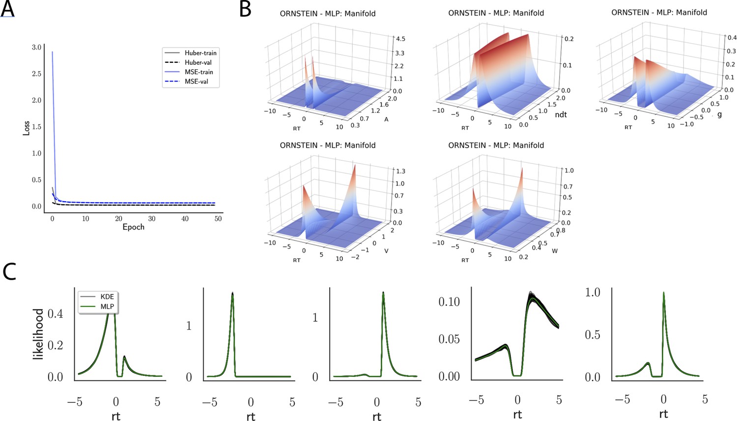
Likelihoods and manifolds: Ornstein.
(A) shows the training and validation loss for Huber as well as MSE for the Ornstein model. Training was driven by the Huber loss. (B) illustrates the likelihood manifolds by varying one parameter in the trained region. (C) shows multilayered perceptron likelihoods in green on top of a sample of 50 kernel density estimate-based empirical likelihoods derived from 100k samples each.
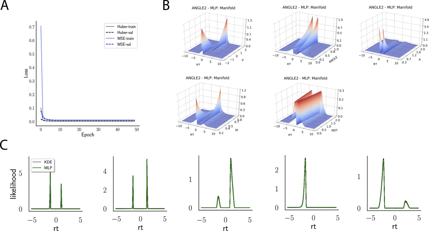
Appendix 1—figure 6
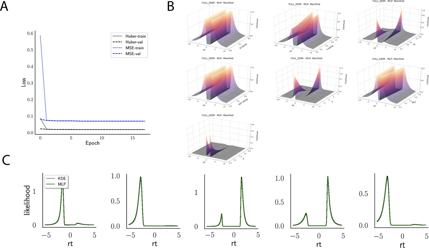
Likelihoods and manifolds: full-DDM.
(A) shows the training and validation loss for Huber as well as MSE for the full drift diffusion model. Training was driven by the Huber loss. (B) illustrates the likelihood manifolds by varying one parameter in the trained region. (C) shows multilayered perceptron likelihoods in green on top of a sample of 50 kernel density estimate-based empirical likelihoods derived from 100k samples each.
Tables
Appendix 1—table 1
Parameter recovery for a variety of test bed models.
| DDM | N | v | a | w | ndt | |||||||||
|---|---|---|---|---|---|---|---|---|---|---|---|---|---|---|
| MLP | 1024 | 1.0 | 1.0 | 0.99 | 1 | |||||||||
| 4096 | 1.0 | 1.0 | 0.99 | 1 | ||||||||||
| CNN | 1024 | 1 | 0.94 | 0.98 | 1 | |||||||||
| 4096 | 1 | 1 | 0.99 | 1 | ||||||||||
| DDM-SDV | v | a | w | ndt | sdv | |||||||||
| MLP | 1024 | 0.95 | 0.94 | 0.96 | 1 | 0.57 | ||||||||
| 4096 | 0.94 | 0.95 | 0.97 | 1 | 0.58 | |||||||||
| CNN | 1024 | 0.98 | 0.97 | 0.98 | 1 | 0.79 | ||||||||
| 4096 | 0.99 | 0.98 | 0.99 | 1 | 0.87 | |||||||||
| LC | v | a | w | ndt | θ | |||||||||
| MLP | 1024 | 0.99 | 0.93 | 0.97 | 1 | 0.98 | ||||||||
| 4096 | 0.99 | 0.94 | 0.98 | 1 | 0.97 | |||||||||
| CNN | 1024 | 0.96 | 0.94 | 0.97 | 1 | 0.97 | ||||||||
| 4096 | 0.97 | 0.94 | 0.98 | 1 | 0.97 | |||||||||
| OU | v | a | w | ndt | g | |||||||||
| MLP | 1024 | 0.98 | 0.89 | 0.98 | 0.99 | 0.12 | ||||||||
| 4096 | 0.99 | 0.79 | 0.95 | 0.99 | 0.03 | |||||||||
| CNN | 1024 | 0.99 | 0.94 | 0.97 | 1 | 0.41 | ||||||||
| 4096 | 0.99 | 0.95 | 0.98 | 1 | 0.45 | |||||||||
| Levy | v | a | w | ndt | α | |||||||||
| MLP | 1024 | 0.96 | 0.94 | 0.84 | 1 | 0.33 | ||||||||
| 4096 | 0.97 | 0.91 | 0.61 | 1 | 0.2 | |||||||||
| CNN | 1024 | 0.99 | 0.97 | 0.9 | 1 | 0.71 | ||||||||
| 4096 | 0.99 | 0.98 | 0.95 | 1 | 0.8 | |||||||||
| Weibull | v | a | w | ndt | α | β | ||||||||
| MLP | 1024 | 0.99 | 0.82 | 0.96 | 1 | 0.2 | 0.43 | |||||||
| 4096 | 0.99 | 0.8 | 0.98 | 0.99 | 0.26 | 0.41 | ||||||||
| CNN | 1024 | 0.98 | 0.91 | 0.96 | 1 | 0.4 | 0.69 | |||||||
| 4096 | 0.98 | 0.91 | 0.97 | 1 | 0.37 | 0.63 | ||||||||
| Full-DDM | v | a | w | ndt | dw | sdv | dndt | |||||||
| MLP | 1024 | 0.95 | 0.94 | 0.88 | 1 | 0 | 0.28 | 0.47 | ||||||
| 4096 | 0.93 | 0.94 | 0.88 | 1 | 0 | 0.25 | 0.38 | |||||||
| CNN | 1024 | 0.98 | 0.98 | 0.93 | 1 | 0 | 0.62 | 0.79 | ||||||
| 4096 | 0.99 | 0.99 | 0.97 | 1 | 0 | 0.8 | 0.91 | |||||||
| Race 3 | v0 | v1 | v2 | a | w0 | w1 | w2 | ndt | ||||||
| CNN | 1024 | 0.88 | 0.86 | 0.89 | 0.19 | 0.49 | 0.51 | 0.5 | 0.99 | |||||
| 4096 | 0.93 | 0.91 | 0.93 | 0.18 | 0.49 | 0.47 | 0.47 | 1 | ||||||
| Race 4 | v0 | v1 | v2 | v3 | a | w0 | w1 | w2 | w3 | ndt | ||||
| CNN | 1024 | 0.73 | 0.68 | 0.71 | 0.73 | 0.11 | 0.49 | 0.5 | 0.48 | 0.49 | 0.99 | |||
| 4096 | 0.79 | 0.76 | 0.77 | 0.81 | 0.18 | 0.5 | 0.5 | 0.51 | 0.55 | 0.99 | ||||
| LCA 3 | v0 | v1 | v2 | a | w0 | w1 | w2 | g | b | ndt | ||||
| CNN | 1024 | 0.58 | 0.56 | 0.58 | 0.47 | 0.7 | 0.72 | 0.68 | 0.27 | 0.57 | 1 | |||
| 4096 | 0.51 | 0.5 | 0.52 | 0.44 | 0.67 | 0.67 | 0.66 | 0.23 | 0.52 | 1 | ||||
| LCA 4 | v0 | v1 | v2 | v3 | a | w0 | w1 | w2 | w3 | g | b | ndt | ||
| CNN | 1024 | 0.5 | 0.46 | 0.54 | 0.51 | 0.51 | 0.71 | 0.69 | 0.69 | 0.67 | 0.18 | 0.7 | 0.99 | |
| 4096 | 0.42 | 0.42 | 0.46 | 0.42 | 0.52 | 0.67 | 0.63 | 0.68 | 0.65 | 0.15 | 0.64 | 1 | ||
| MLP: multilayered perceptron; CNN: convolutional neural network; DDM: drift diffusion model; LC: linear collapse; LCA: leaky competing accumulator. | ||||||||||||||
Additional files
Download links
A two-part list of links to download the article, or parts of the article, in various formats.
Downloads (link to download the article as PDF)
Open citations (links to open the citations from this article in various online reference manager services)
Cite this article (links to download the citations from this article in formats compatible with various reference manager tools)
Likelihood approximation networks (LANs) for fast inference of simulation models in cognitive neuroscience
eLife 10:e65074.
https://doi.org/10.7554/eLife.65074


