Learning to stand with unexpected sensorimotor delays
- School of Physical Education, Sport, and Exercise Sciences, University of Otago, New Zealand
- Department of Neuroscience, Erasmus MC, University Medical Center Rotterdam, Netherlands
- School of Kinesiology, University of British Columbia, Canada
- Faculty of Kinesiology, University of Calgary, Canada
- Hotchkiss Brain Institute, Canada
- Faculty of Kinesiology, University of New Brunswick, Canada
- Djavad Mowafaghian Centre for Brain Health, University of British Columbia, Canada
- Institute for Computing, Information and Cognitive Systems, University of British Columbia, Canada
Figures
Figure 1
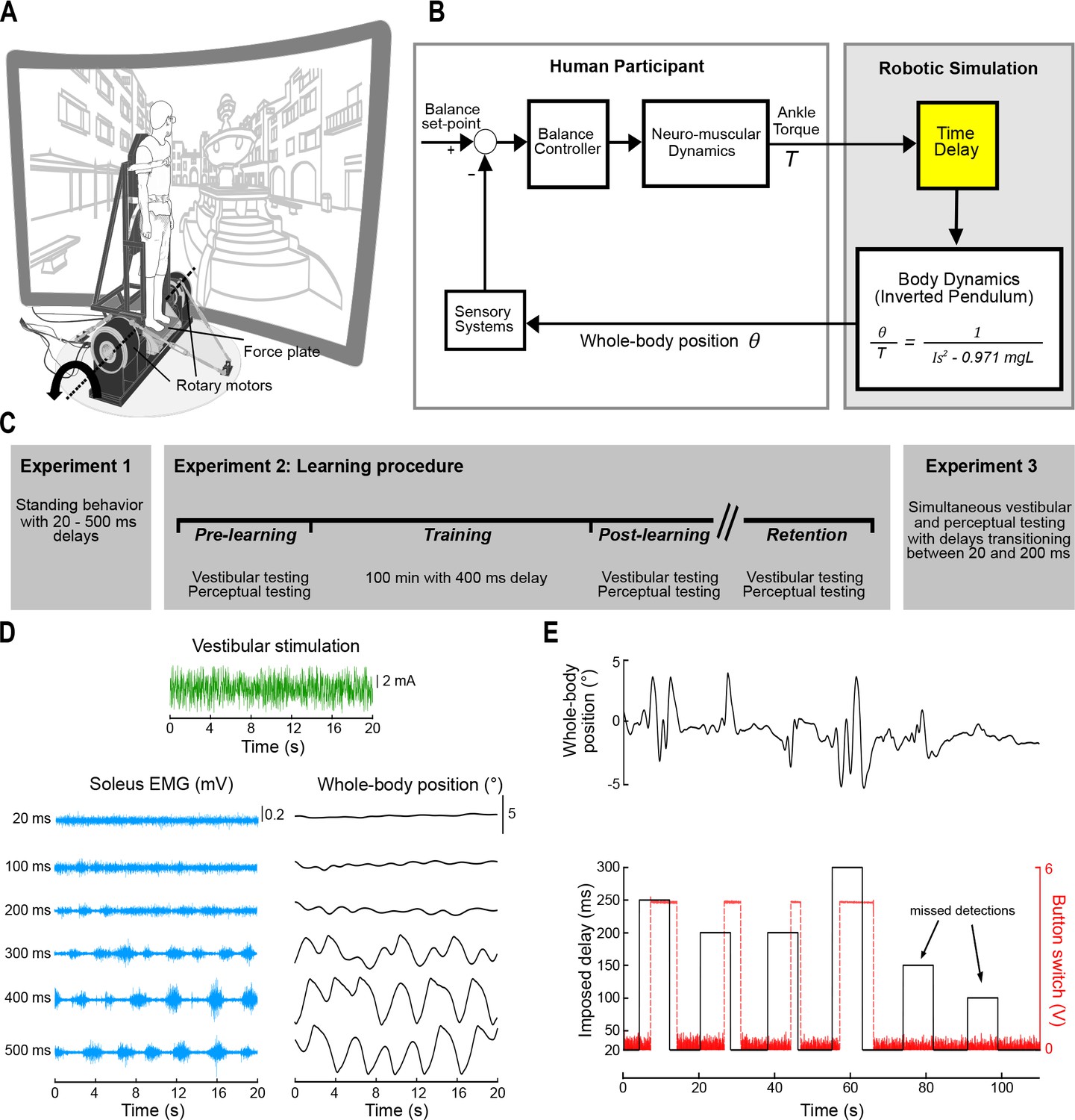
Experimental setup and block diagram of robotic simulation.
(A) The participant stood on a force plate mounted to an ankle-tilt platform and was securely strapped to a rigid backboard. The ankle-tilt platform and backboard were independently controlled by rotary motors. In all experiments, the ankle-tilt platform was held at horizontal (earth-fixed reference) while the backboard rotated the participant in the anteroposterior plane. Motion of the backboard was controlled by ankle torques exerted on the force plate based on the mechanics of an inverted pendulum. The backboard rotated about an axis that passed through the participant’s ankles (dashed line). Participants wore 3D goggles and viewed a virtual scene of a courtyard. (B) Participants balanced the robotic simulator as it operated with a 20–500 ms delay. Torque signals (T) from the force plate were buffered in the robotic simulation computer model such that angular rotation of the whole body (θ) about the ankle joint could be delayed. (C) Experimental design. Experiment 1 involved testing standing balance when naïve participants (n = 13) were first exposed to delays. Experiment 2 involved learning to balance with delays and was performed in two groups: vestibular testing and perceptual testing (see Experiment 2 methods). All participants who performed the learning experiments (vestibular testing group, n = 8; perceptual testing group, n = 8) completed an identical training protocol. The vestibular and perceptual tests were completed before, immediately after, and ~3 months following training. Training was completed over 5 days, in which the participant balanced the robotic simulator with a 400 ms delay (20 min per day). Experiment 3 tested a new group of participants (n = 7) and evaluated the time-dependent attenuation in vestibular-evoked responses together with changes in sway behavior and perception of unexpected balance motion. Trials in Experiment 3 were of similar design to perceptual testing in Experiment 2 (see panel E), except that the robot only transitioned between baseline (20 ms) and 200 ms delays. (D) Raw data of a sample participant from Experiment 2 vestibular testing. The participant was exposed to electrical vestibular stimulation while balancing the robotic simulator as it operated at fixed delays. Raw traces of the vestibular stimulus (green), soleus muscle EMG (blue), and whole-body position (black) are shown for a single trial at each delay condition. (E) During perceptual testing (Experiments 2 and 3), the participant balanced the robotic balance simulator and held a button switch. Delays were manipulated in the robotic balance simulation and the participant was required to press and hold the button when unexpected balance motion was detected. Raw data traces of whole-body position (black, upper trace), imposed simulation delay (black, lower trace), and the button switch (red) are shown during a perceptual trial from Experiment 2. Black arrows indicate examples of imposed delays that did not elicit a perceptual detection. Figure 1A was adapted from Shepherd, 2014.
Figure 2
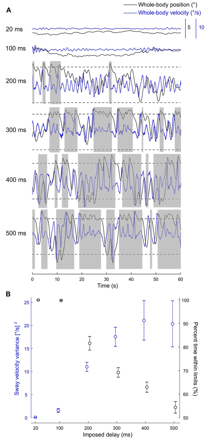
Standing balance behavior with delays.
(A) Experiment 1: raw traces of body position (black) and velocity (blue) for a single participant balancing on the robotic simulator for 60 s at different imposed delay conditions. Dashed lines represent the virtual position limits (6° anterior, 3° posterior). Sway velocity variance was calculated over 2 s windows (extracted by taking segments when sway was within balance limits for at least two continuous seconds) and the resulting data were averaged to provide a single estimate per participant and delay (see Materials and methods). Data that are not grayed out represent periods where there is at least two continuous seconds of balance within the virtual position limits. The percentage of trial time participant’s whole-body position remained within the limits was also quantified. (B) Group (n = 13) averages of sway velocity variance (blue) and percent time within balance limits (black). Error bars represent ± s.e.m.
Figure 3
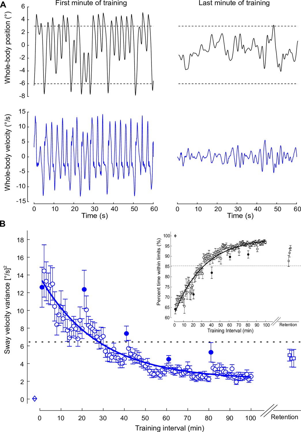
Standing balance behavior during the training protocol.
(A) Whole-body position (°; black) and velocity (°/s; blue) traces of a representative participant when balancing in the first (left) and last (right) minute of training. During training trials, the robotic simulator operated with a 400 ms delay. (B) Average sway velocity variance and percentage of time spent within the virtual balance limits (inset) estimated over 1 min intervals during the 400 ms delay training (open circles) from all participants who completed the training protocol (n = 16). The first interval for each training session is represented by filled circles. Data from vestibular testing and perceptual testing groups were combined because both groups performed the same training protocol. Sway velocity variance progressively decreased and percentage of the interval time within the virtual limits progressively increased with each session of training (one session = 20 intervals). The solid lines show the fitting of sway velocity variance and percentage within virtual balance limits to a first-order exponential function using a least-square method: . For sway velocity variance, a = 11.61, b = 27.86, and c = 2.17; for percentage time within balance limits, a = –37.38, b = 32.45, and c = 99.12. The dashed horizontal lines represent the values at the estimated time constants. Data for the first minute of standing at 20 ms (open diamond) and the three minutes at 3 months after training (retention) at the 400 ms delay (open squares) are also presented. Error bars represent the s.e.m. for all data.
Figure 4
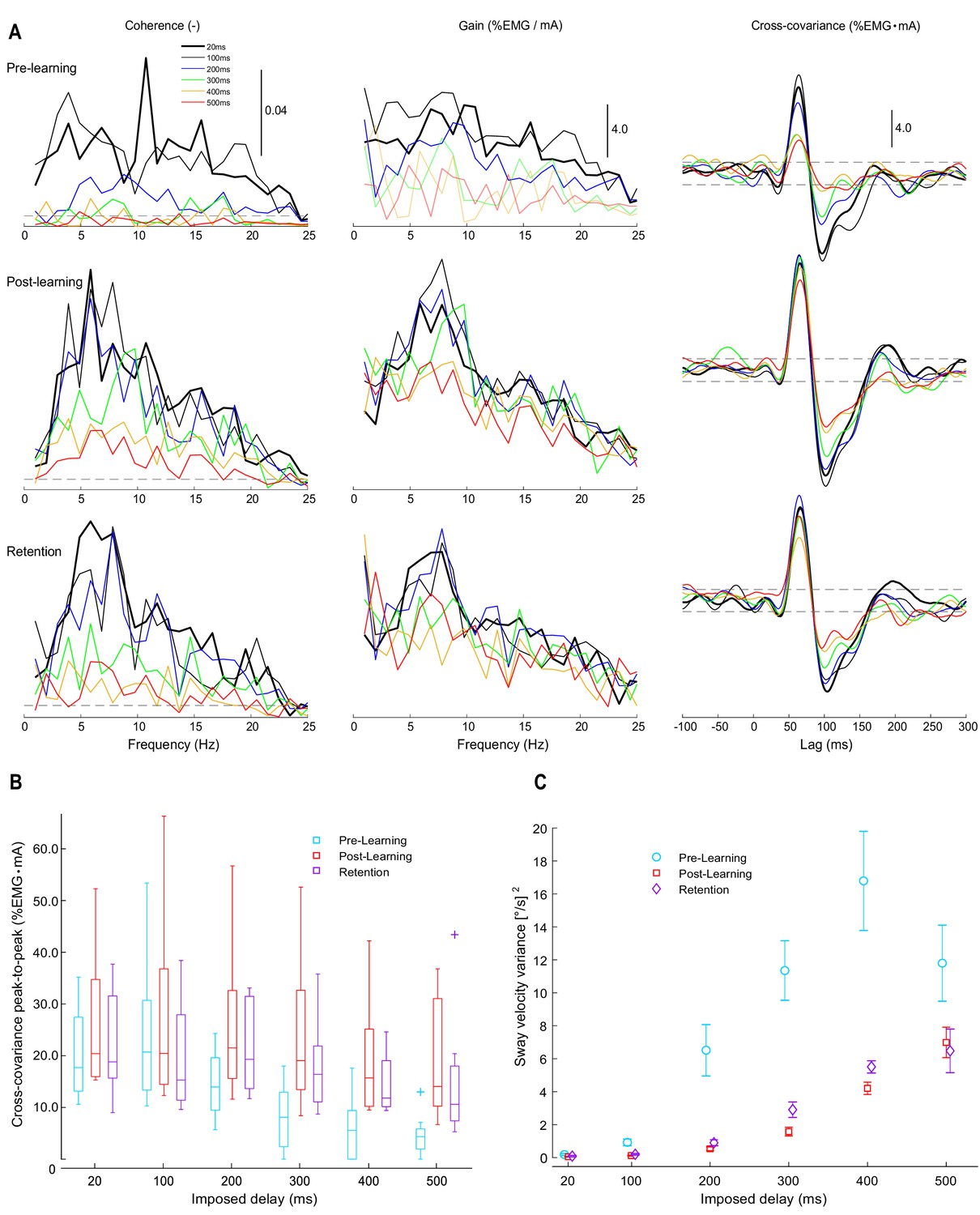
Experiment 2 vestibular-evoked muscle responses.
Data are from pre-learning (n = 8), post-learning (n = 8), and retention (n = 7) conditions. (A) Coherence, gain, and cross-covariance between vestibular stimuli and rectified soleus EMG activity were calculated from the data concatenated from all participants. Estimates are presented from all six delay conditions (see legend). Horizontal dashed lines represent 95% confidence limits for coherence and the 95% confidence intervals for cross-covariance. Note that gain estimates are only reliable at frequencies with significant coherence; therefore, at delays ≥ 300 ms, where coherence falls below significance at most frequency points, the corresponding gain in the pre-learning condition was plotted using light lines. EMG was scaled by baseline EMG from each testing session (see Materials and methods), resulting in units for gain and cross-covariance of %EMG/mA and %EMG mA, respectively. (B) Group cross-covariance amplitudes (peak-to-peak) plotted relative to imposed delay. Across pooled estimates and group data, vestibular responses attenuated with increasing imposed delays and their amplitudes partially recovered after training. (C) Average sway velocity variance during vestibular stimulation trials. Non-normally distributed group data (vestibular response amplitudes) are plotted as medians (horizontal lines in boxes), 25 and 75 percentiles (boxes) and extreme data points (error bars). Normally distributed data (sway velocity variance) are presented as means with s.e.m (error bars).
Figure 5
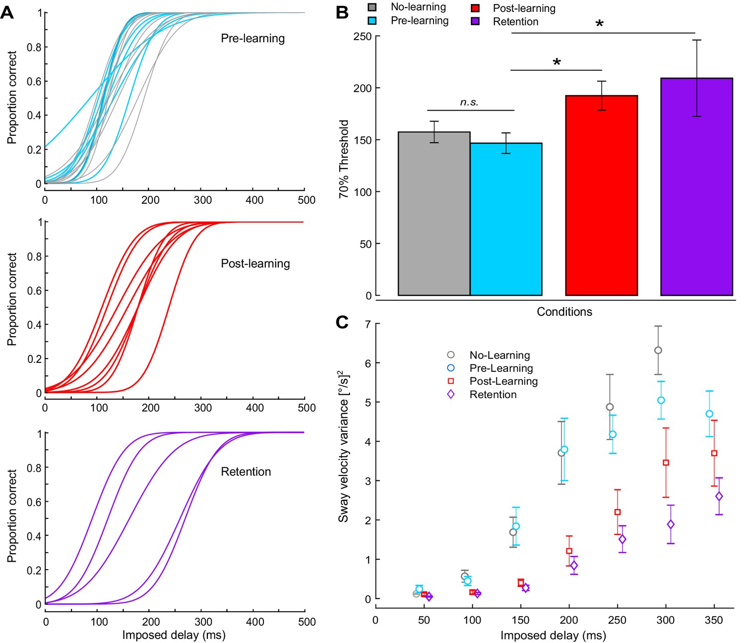
Experiment 2 perceptual testing and standing behavior results.
(A) A Bayesian estimation procedure was used to fit sigmoidal functions to perceptual responses. The proportion of correct responses (i.e., button pressed during delay period) was calculated for each participant at each delay level. Individual psychometric functions are shown for all participants. The top panel shows participants tested before training (n = 18), with 10 participants who did not participate in the learning procedure shown in gray. The middle panel shows post-learning (n = 8), and the bottom panel shows retention results (n = 5). (B) Average 70% interpolated threshold for pre, post, and retention conditions. Perceptual thresholds increased following training, such that larger imposed delays were needed to elicit perceptual detections. (C) Average velocity variance for different delays. Error bars indicate s.e.m.
Figure 6
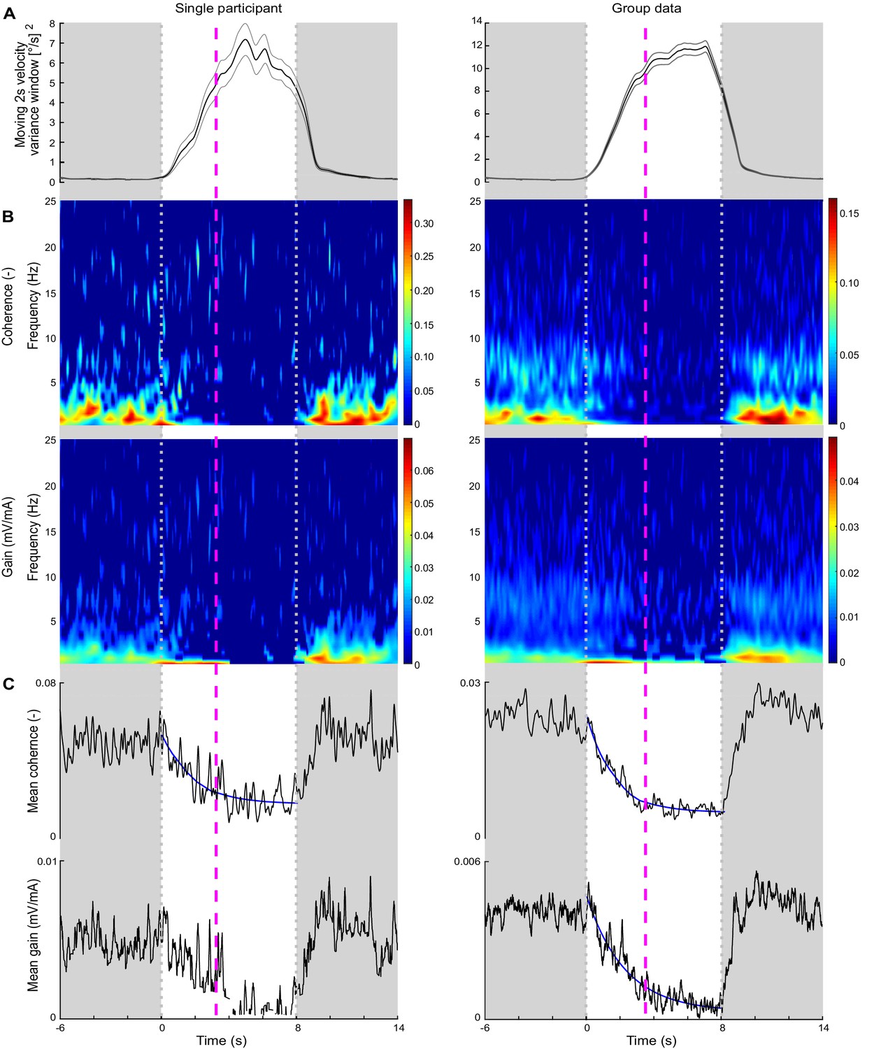
Experiment 3 sway velocity variance, time-varying electrical vestibular stimulus-electromyography (EVS-EMG) coherence and gain, and perceptual detection time during delay transitions.
Data are presented across transition periods where time zero represents the transition point from baseline (20 ms) to 200 ms delayed balance control, which lasted for 8 s (between grayed out areas) and returned to baseline. Data are presented for a representative participant (left) and the group data (right; n = 7) using only data from transitions that were perceived as unexpected and the button was pressed after the delay was introduced (single participant: 77, group: 489). (A) Average (black line) 2 s sliding window of velocity variance over transitions with ±s.e.m. (gray lines). Time-varying variance was calculated using the movvar MATLAB function, which calculated variance over 2 s segments using a sliding window. The velocity variance trace begins to decline prior to the end of the delay period because the sliding window starts estimating variances from data points both during and after the delay. (B) Time-frequency plots of EVS-EMG coherence and gain (i.e., vestibular-evoked muscle responses) during the delay transition. For illustrative purposes, and because gain values are not reliable when coherence is below the significance threshold, we set coherence and gain data points where coherence was non-significant (i.e., below 99% confidence limit) to zero (dark blue). (C) Mean time-dependent EVS-EMG coherence and gain across the 0.5–25 Hz frequency range. For each participant and group data, an exponential decay function: was fit to the average coherence over the 8 s period during which the 200 ms delay was present. For gain, we removed values corresponding to non-significant coherence (see single participant trace) and only fit an exponential function to the group mean gain estimate. The average perceptual detection times for the representative participant (3.2 s) and group data (3.4 s) are indicated by the dashed magenta lines, and at these times, vestibulomuscular coherence had attenuated by 83% and 90%, respectively. Group mean gain attenuated by 73% at the group average perceptual detection time.
Author response image 1
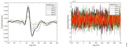
Pooled non-normalized cross-covariance (left) and impulse response (right) estimates from pre-learning data set sampled at 2000 Hz.
Estimates were calculated by concatenating data from all eight participants.
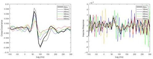
Author response image 2

Pooled non-normalized cross-covariance (left) and impulse response (right) functions from pre-learning data, originally sampled at 2000Hz and then down-sampled offline to 50Hz.
Note that cross-covariance and impulse response functions now provide similar results after down-sampled to 50Hz. Both responses, however, have poor resolution when compared to the original cross-covariance (Response Figure 1; 2000Hz).
Author response image 3
Pooled non-normalized cross-covariance (left) and impulse response (right) functions from pre-learning data, originally sampled at 2000Hz and then down-sampled offline to 100Hz.
Note that the impulse response functions already become noisy when the data are downsampled to 100Hz.
Author response image 4
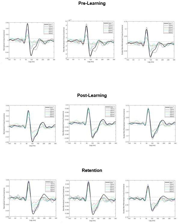
Pooled cross-covariance estimates of vestibular-evoked muscle responses.
Normalized responses (left), non-normalized responses (center) and scaled non-normalized responses (right). All three approaches produce a similar outcome: vestibular-evoked response amplitudes attenuate with increasing imposed delays (particularly in pre-learning) and partially return to baseline levels after training (observed in post-learning and retention). Dashed lines are 95% confidence intervals.
Author response image 5

Experiment 3 time-varying EVS-EMG coherence, gain and sway velocity variability during detected (perceived) and missed (not perceived) delay transitions.
Data are presented across transition periods, where the simulation transitioned from baseline to 200 ms delayed balance control, which lasted for 8s (between dashed red vertical lines). Top panel, a comparison of 82 detected and missed transitions vestibular-evoked muscle coherence and gain. Dashed lines represent coherence and gain levels which are 2 standard deviations below the mean levels in the 6 seconds preceding the onset of the delay. Bottom panel, a comparison of sway velocity variance from 82 detected and 82 missed transitions. Thick lines represent the mean with lighter lines representing the s.e.m. For both panels, blue and red traces represent detected and missed transitions, respectively.
Tables
Table 1
Summary of statistical results.
| Delay | Learning | Delay × learning interaction | ||||
|---|---|---|---|---|---|---|
| Variable | F | p | F | p | F | p |
| Sway velocity variance | ||||||
| Exp 1: standing balance trials | F(5,59.15) = 14.98 | < 0.001 | N/A | N/A | N/A | N/A |
| Exp 2: vestibular testing | F(5,111.26) = 33.89 | < 0.001 | F(2,113.19) = 46.65 | < 0.001 | F(10,111.25) = 5.72 | < 0.001 |
| Exp 2: perceptual testing | F(6,118.83) = 31.00 | < 0.001 | F(2,121.47) = 25.82 | < 0.001 | F(12,118.83) = 2.08 | = 0.023 |
| Other variables | ||||||
| Exp 1: percent within limits | F(5,60) = 127.48 | < 0.001 | N/A | N/A | N/A | N/A |
| Exp 2: cross-covariance | W(5) = 1158.86 | < 0.001 | W(2) = 70.57 | < 0.001 | W(7) = 90.89 | < 0.001 |
| Exp 2: perceptual threshold | N/A | N/A | F(2,11.84) = 7.52 | = 0.008 | N/A | N/A |
-
For Exp 2, vestibular cross-covariance responses (peak-to-peak amplitudes) were analyzed using an ordinal logistic regression after rank transforming the data.
Table 2
Vestibular response magnitude and sway behavior from vestibular stimulation trials in Experiment 2 vestibular testing.
| Delay (ms) | 20 | 100 | 200 | 300 | 400 | 500 |
|---|---|---|---|---|---|---|
| Pre-learning (n = 8) | ||||||
| Cross-cov. (%EMG·mA) | 17.7/16.0 | 20.7/18.8 | 14.0/11.0 | 8.10/12.4 | 5.54/10.9 | 4.35/5.50 |
| Sway velocity variance [°/s]2 | 0.18 ± 0.17 | 0.93 ± 0.58 | 6.52 ± 4.40 | 11.35 ± 5.10 | 16.79 ± 8.51 | 11.80 ± 6.53 |
| Post-learning (n = 8) | ||||||
| Cross-cov. (%EMG·mA) | 20.4/23.2 | 20.4/26.7 | 21.5/19.6 | 19.1/20.5 | 15.7/16.0 | 14.1/21.4 |
| Sway velocity variance [°/s]2 | 0.05 ± 0.05 | 0.13 ± 0.09 | 0.54 ± 0.32 | 1.58 ± 0.74 | 4.20 ± 1.05 | 6.99 ± 2.61 |
| Retention (n = 7) | ||||||
| Cross-cov. (%EMG·mA) | 18.8/20.0 | 15.3/17.6 | 19.3/20.1 | 16.4/12.5 | 11.8/9.16 | 10.6/13.3 |
| Sway velocity variance [°/s]2 | 0.09 ± 0.11 | 0.20 ± 0.12 | 0.90 ± 0.48 | 2.91 ± 1.25 | 5.51 ± 0.98 | 6.48 ± 3.51 |
Table 3
Perceptual detection rates and sway behavior from perceptual testing in Experiment 2.
| Delay (ms) | 50 | 100 | 150 | 200 | 250 | 300 | 350 |
|---|---|---|---|---|---|---|---|
| No learning (n = 10)* | |||||||
| Used trials (out of 200) | 197 | 194 | 195 | 196 | 195 | 198 | N/A |
| Detections (% detected) | 8 (4%) | 60 (31%) | 128 (66%) | 172 (88%) | 186 (95%) | 198 (100%) | N/A |
| Sway velocity variance [°/s]2 | 0.12 ± 0.05 | 0.57 ± 0.48 | 1.69 ± 1.21 | 3.71 ± 2.52 | 4.87 ± 2.62 | 6.32 ± 1.95 | N/A |
| Detection time (s) | 3.8 ± 2.0 | 4.7 ± 2.0 | 4.0 ± 1.9 | 3.5 ± 1.8 | 2.9 ± 1.5 | 2.6 ± 1.2 | N/A |
| Pre-learning (n = 8) | |||||||
| Used trials (out of 160) | 148 | 151 | 147 | 147 | 150 | 151 | 152 |
| Detections (% detected) | 20 (14%) | 46 (30%) | 111 (76%) | 132 (90%) | 146 (97%) | 151 (100%) | 152 (100%) |
| Sway velocity variance [°/s]2 | 0.24 ± 0.27 | 0.45 ± 0.33 | 1.84 ± 1.36 | 4.01 ± 2.33 | 4.18 ± 1.38 | 5.09 ± 1.46 | 4.70 ± 1.64 |
| Detection time (s) | 4.1 ± 2.1 | 3.7 ± 1.9 | 3.6 ± 1.8 | 3.2 ± 1.6 | 2.9 ± 1.6 | 2.4 ± 1.2 | 2.3 ± 1.1 |
| Post-learning (n = 8) | |||||||
| Used trials (out of 160) | 157 | 156 | 157 | 156 | 157 | 157 | 151 |
| Detections (% detected) | 16 (10%) | 23 (15%) | 52 (33%) | 101 (65%) | 136 (87%) | 153 (97%) | 151 (100%) |
| Sway velocity variance [°/s]2 | 0.11 ± 0.10 | 0.16 ± 0.13 | 0.40 ± 0.26 | 1.34 ± 1.09 | 2.20 ± 1.61 | 3.02 ± 2.33 | 3.70 ± 2.37 |
| Detection time (s) | 4.2 ± 2.0 | 3.8 ± 2.4 | 4.1 ± 1.7 | 3.9 ± 1.7 | 3.4 ± 1.8 | 2.7 ± 1.3 | 2.2 ± 1.1 |
| Retention (n = 5) | |||||||
| Used trials (out of 100) | 96 | 93 | 98 | 98 | 96 | 98 | 92 |
| Detections (% detected) | 8 (8%) | 21 (23%) | 40 (41%) | 50 (51%) | 71 (74%) | 84 (86%) | 92 (100%) |
| Sway velocity variance [°/s]2 | 0.05 ± 0.03 | 0.13 ± 0.06 | 0.27 ± 0.15 | 0.84 ± 0.51 | 1.51 ± 0.76 | 1.89 ± 1.09 | 2.60 ± 1.05 |
| Detection time (s) | 5.0 ± 1.7 | 4.2 ± 2.0 | 4.2 ± 2.2 | 3.8 ± 2.0 | 3.4 ± 1.8 | 3.1 ± 1.8 | 3.1 ± 1.4 |
-
Sway velocity variance and detection time are presented as mean ± SD.
-
*No learning group is an independent sample of participants that were not exposed to a 350 ms delay.
Additional files
Download links
A two-part list of links to download the article, or parts of the article, in various formats.
Downloads (link to download the article as PDF)
Open citations (links to open the citations from this article in various online reference manager services)
Cite this article (links to download the citations from this article in formats compatible with various reference manager tools)
Learning to stand with unexpected sensorimotor delays
eLife 10:e65085.
https://doi.org/10.7554/eLife.65085


