Allosteric conformational ensembles have unlimited capacity for integrating information
- Department of Systems Biology, Harvard Medical School, United States
- Institute for Medical Engineering and Science, Department of Biological Engineering, Massachusetts Institute of Technology, United States
- Infectious Disease and Microbiome Program, Broad Institute of MIT and Harvard, United States
Figures
Figure 1
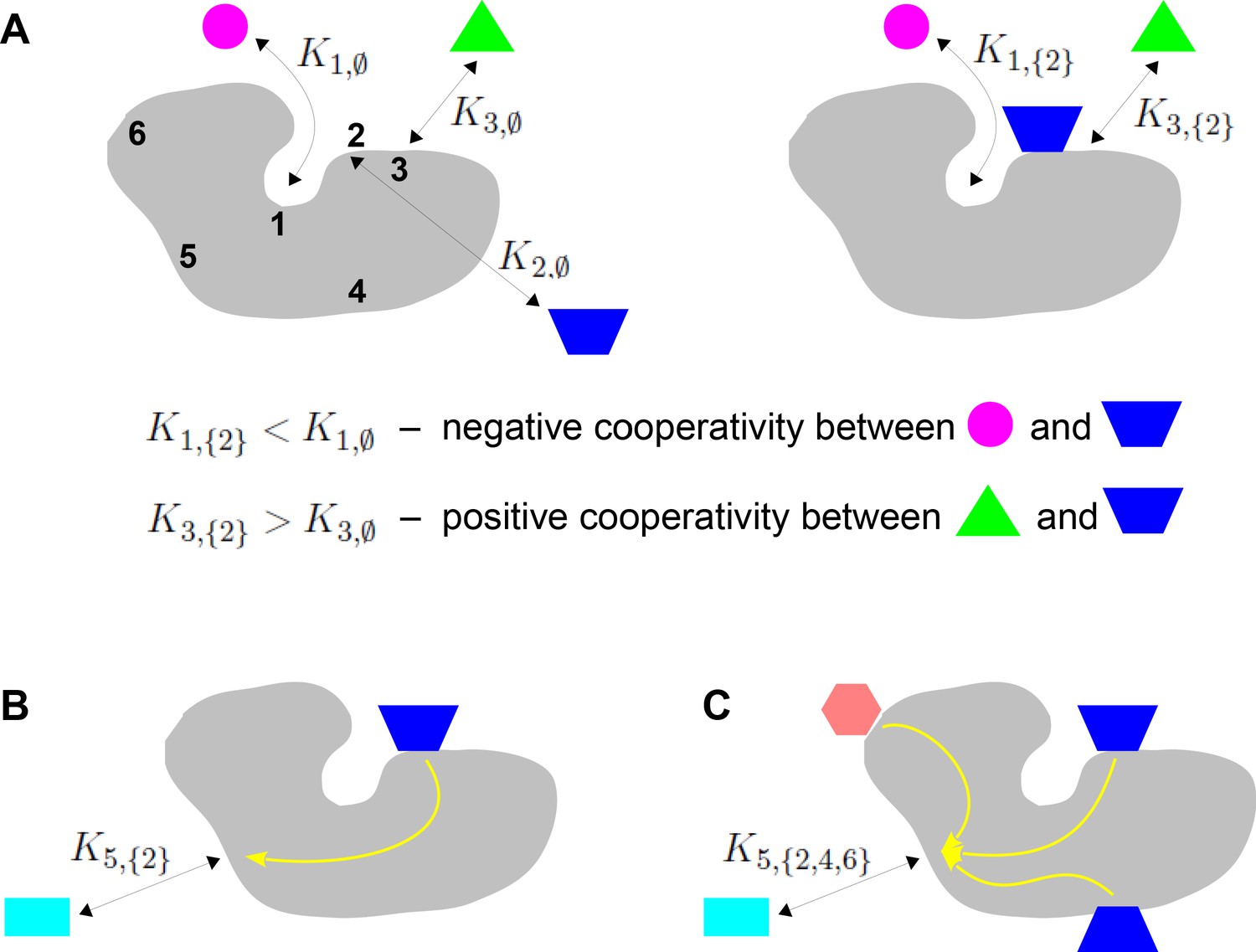
Binding cooperativity.
(A) Pairwise cooperativity by direct interaction on a target molecule (grey). As discussed in the text, the target could be any molecular entity. Left: target molecule with no ligands bound; numbers denote the binding sites. Right: target molecule after binding of blue ligand to site 2. (B) Indirect long-distance pairwise cooperativity, which can arise ‘effectively’ through allostery. (C) Higher-order cooperativity, in which multiple bound sites, 2, 4 and 6, affect binding at site 5.
Figure 2
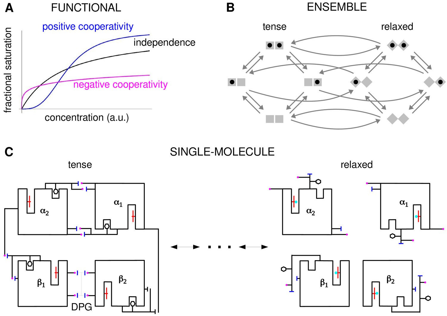
Cooperativity and allostery from three perspectives.
(A) Plots of the binding function, whose shape reflects the interactions between binding sites, as described in the text. (B) The Monod, Wyman and Changeux (MWC) model with a population of dimers in two quaternary conformations, with each monomer having one binding site and ligand binding shown by a solid black disc. The two monomers are considered to be distinguishable, leading to four microstates. Directed arrows show transitions between microstates. This picture anticipates the graph-theoretic representation used later in this paper. (C) Schematic of the end points of the allosteric pathway between the tense, fully deoxygenated and the relaxed, fully oxygenated conformations of a single haemoglobin tetramer, , showing the tertiary and quaternary changes, based on Figure 4 of Perutz, 1970. Haem group (red); oxygen (cyan disc); salt bridge (positive, magenta disc; negative, blue bar); DPG is 2–3-diphosphoglycerate.
Figure 3
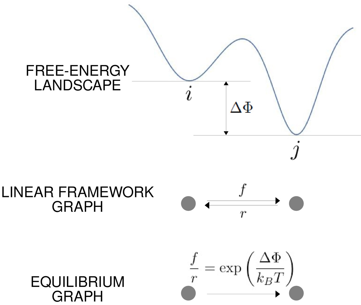
The free-energy landscape and corresponding graphs.
From the top, a hypothetical one-dimensional free-energy landscape, showing two graph vertices, and , as local minima of the free energy; the corresponding linear framework graph showing the edges between and with respective transition rates; the corresponding equilibrium graph whose edge label is the ratio of the transition rates, which is determined by the free-energy difference between the vertices (Equation 1).
Figure 4
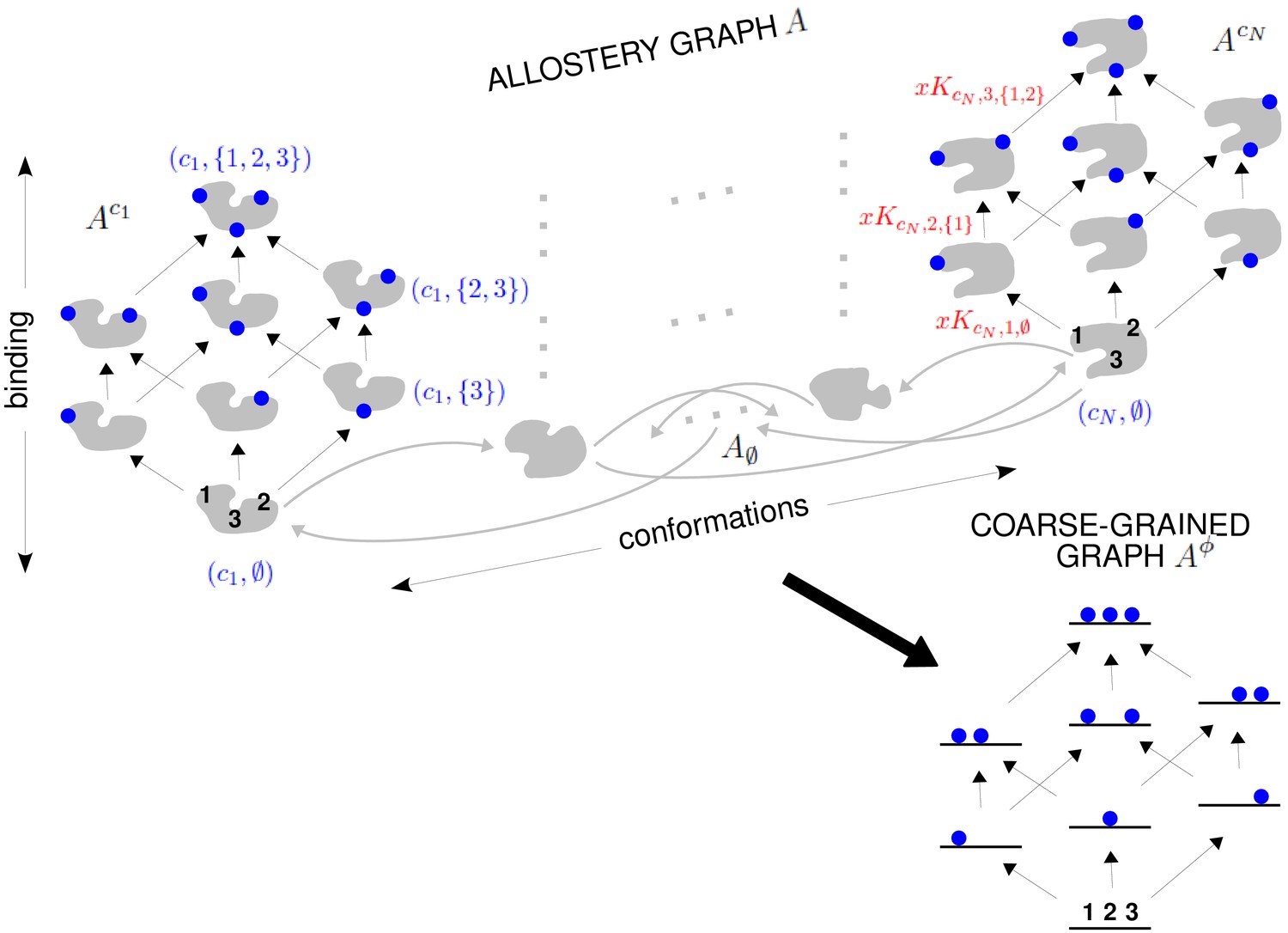
The allostery graph and coarse graining.
A hypothetical allostery graph (top) with three binding sites for a single ligand (blue discs) and conformations, , shown as distinct grey shapes. Binding edges (‘vertical’ in the text) are black and edges for conformational transitions (‘horizontal’) are grey. Similar binding and conformational edges occur at each vertex but are suppressed for clarity. Note that edges are shown in only one direction but are always reversible. All vertical subgraphs, , have the same structure, as seen for the vertical subgraphs, (left) and (right), and all horizontal subgraphs, , also have the same structure, shown schematically for the horizontal subgraph of empty conformation, , at the base. Example notation is given for vertices (blue font) and edge labels (red font), with denoting ligand concentration and sites numbered as shown for vertices and . The coarse-graining procedure coalesces each horizontal subgraph, , into a new vertex and yields the coarse-grained graph, (bottom right), which has the same structure as for any . Further details in the text and the Materials and methods.
Figure 5
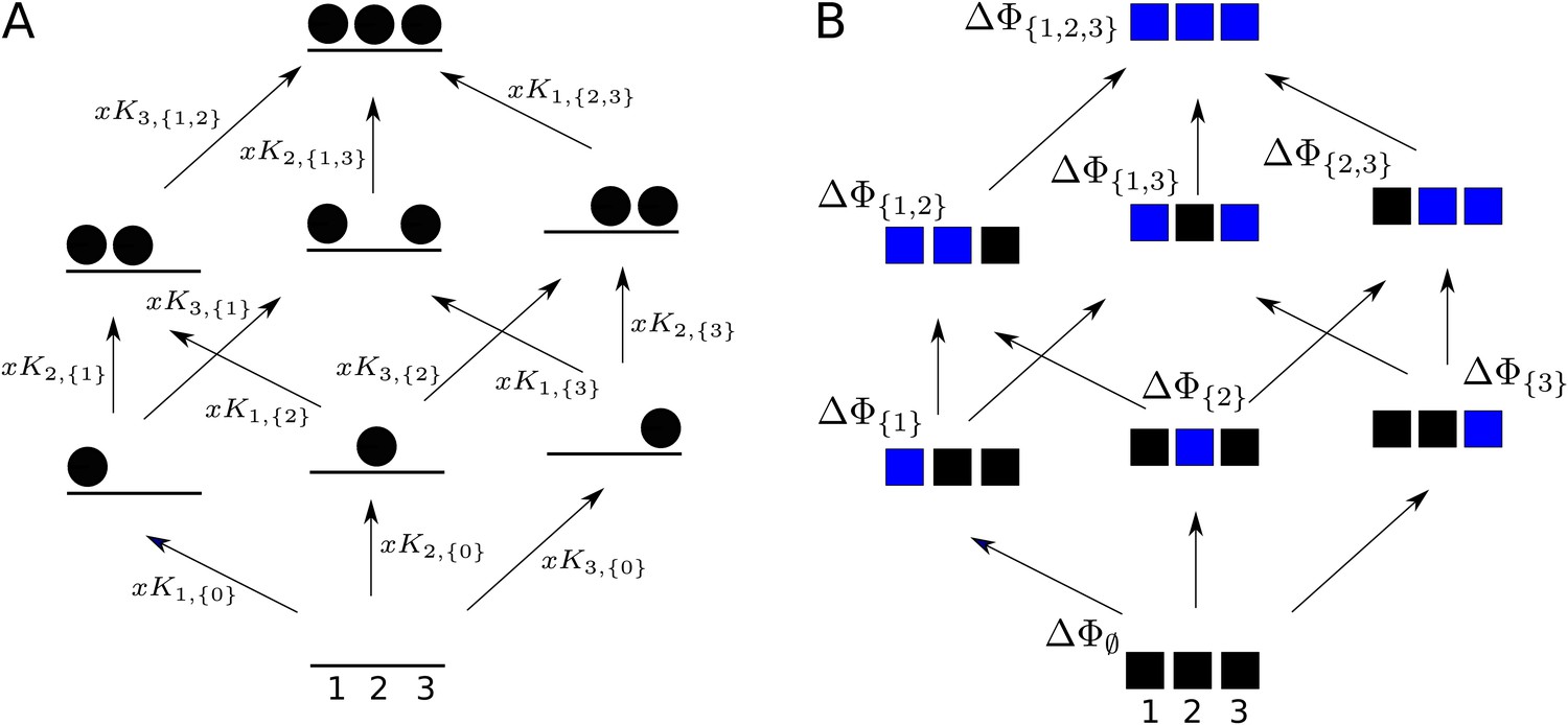
Graphs for defining higher-order measures.
(A) Equilibrium graph, similar to those in Figure 4, for binding of a ligand to three sites on a single conformation, ordered as shown at the base, and annotated with edge labels. The single conformation has been omitted from subscripts for clarity. (B) Directed graph used to define higher-order couplings, for a macromolecule with three sites or modules (solid squares), ordered as shown at the base, with perturbations indicated by blue colour in place of black. Vertices are annotated with the corresponding free energy.
Figure 6
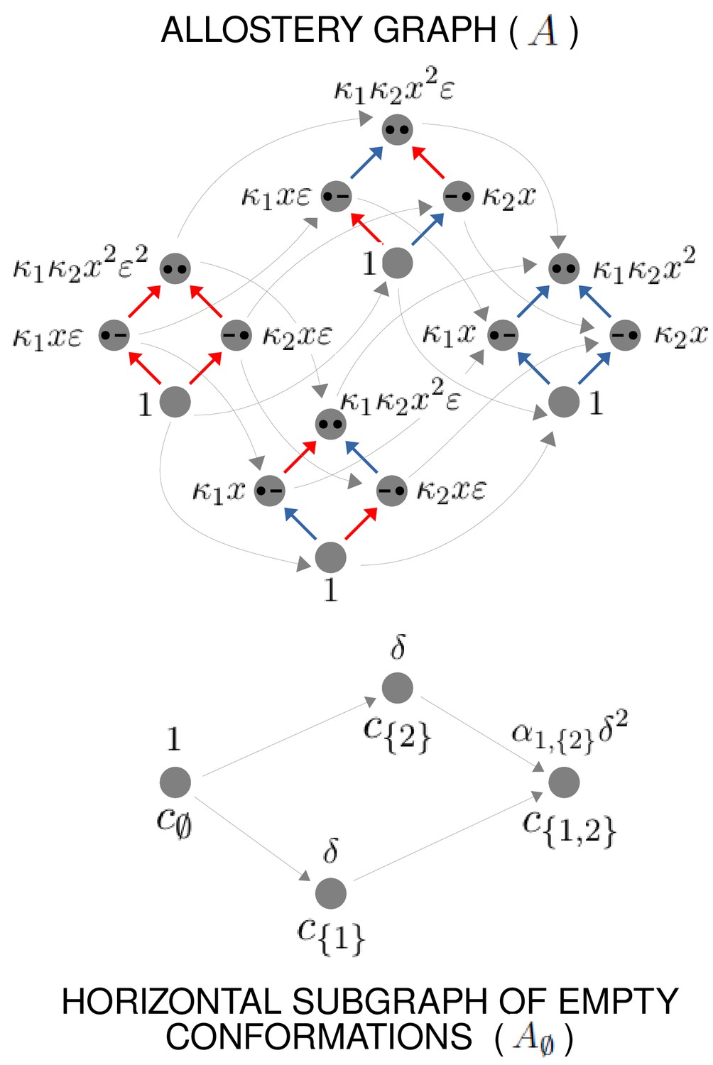
Example allostery graph for the flexibility theorem.
There are sites and conformations, giving a 16-vertex allostery graph (top). Vertices indicate a bound site with a solid black dot and an unbound site with a black dash. Sites are indexed in increasing order, , from left to right. The red vertical binding edges carry a factor of ε in their equilibrium labels; the blue vertical binding edges do not, as specified in the text and Equation 60. The vertices of the allostery graph are annotated with the values of , as specified in the text and Equation 61. The horizontal subgraph of empty conformations is shown at the bottom, with conformations indexed below each vertex by subsets of and annotated above each vertex with the corresponding value of , as specified by Equation 24.
Figure 7
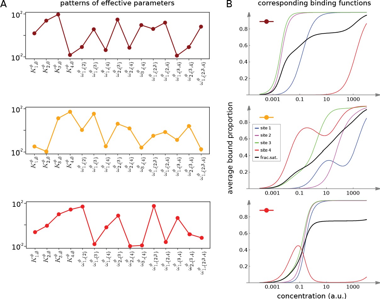
Integrative flexibility of allostery I.
(A) Three choices of effective bare association constants, , in arbitrary units of (concentration)−1, and independent effective higher-order cooperativities , , for , in non-dimensional units, for ligand binding to four sites. Each example is coded by a colour (maroon, orange, red) and exhibits a different pattern of positive and negative effective HOCs. (B) Corresponding plots of average bound proportion at each site (colour coded as in middle inset) and the overall binding function, or fractional saturation, (black), calculated directly from the effective parameters. Note that the latter is always increasing; see the text for more details.
Figure 8
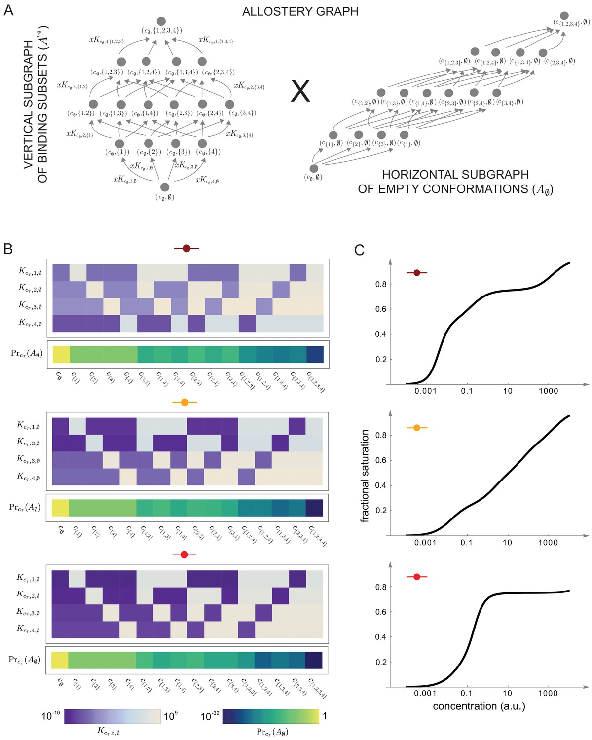
Integrative flexibility of allostery II.
(A) The allostery graph, , which implements the choices of effective higher-order cooperativities (HOCs) in Figure 7, shown as the product of the vertical subgraph of binding patterns at conformation , , and the horizontal subgraph of empty conformations, . As required in the proof of the flexibility theorem, both conformations and binding subsets are indexed by subsets of , where is the number of binding sites. Since for the effective HOCs in Figure 7, there are 16 binding subsets and 16 conformations, . (B) Intrinsic bare association constants, , in each conformation, in arbitrary units of (concentration)−1, and the probability distribution on the subgraph of empty conformations, , for the allostery graph in (A), giving the three choices of effective parameters in Figure 7A to an accuracy of 0.01 (Materials and methods), colour coded on a log scale as shown in the respective legends below. (C) Overall binding functions for the three parameterised ensembles in (B) (black curves), overlaid on the overall binding functions from Figure 7B (red curves), which were calculated from the effective parameters. The match is too close for the red curves to be visible. Numerical values are given in the Materials and methods. Calculations were undertaken in a Mathematica notebook, available on request.
Figure 9
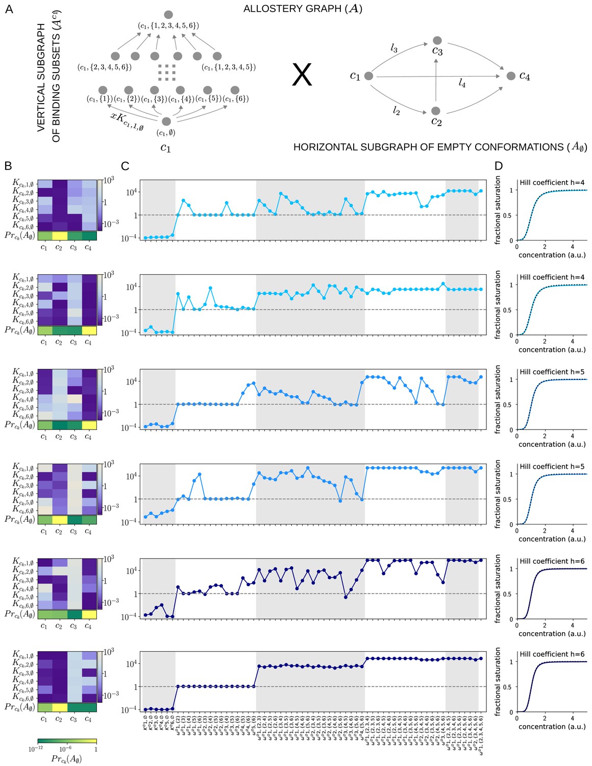
Allosteric ensembles for Hill functions.
(A) Allostery graph, , for representing Hill functions with six binding sites and four conformations, shown as the product of the vertical subgraph of binding subsets and the horizontal subgraph of empty conformations. Some vertices are annotated and some edges are labelled; the edge labels, and , on the horizontal subgraph are the independent labels coming from a spanning tree used in the algorithm described in the text. (B) Intrinsic bare association constants in each conformation, in arbitrary units of (concentration)−1 colour coded in the vertical bar on the right, and the probability distribution on the subgraph of empty conformations, colour coded in the horizontal bar at the bottom. (C) Corresponding effective association constants in arbitrary units of (concentration)−1 and the non-dimensional independent effective higher-order cooperativities arising from the ensemble. (D) Corresponding binding functions (blue curves) overlaid on the Hill function (black dashes) with the indicated Hill coefficient, . Two sets of parameter values are shown, with the same shade of blue, for each Hill coefficient , 5 and 6.
Figure 10
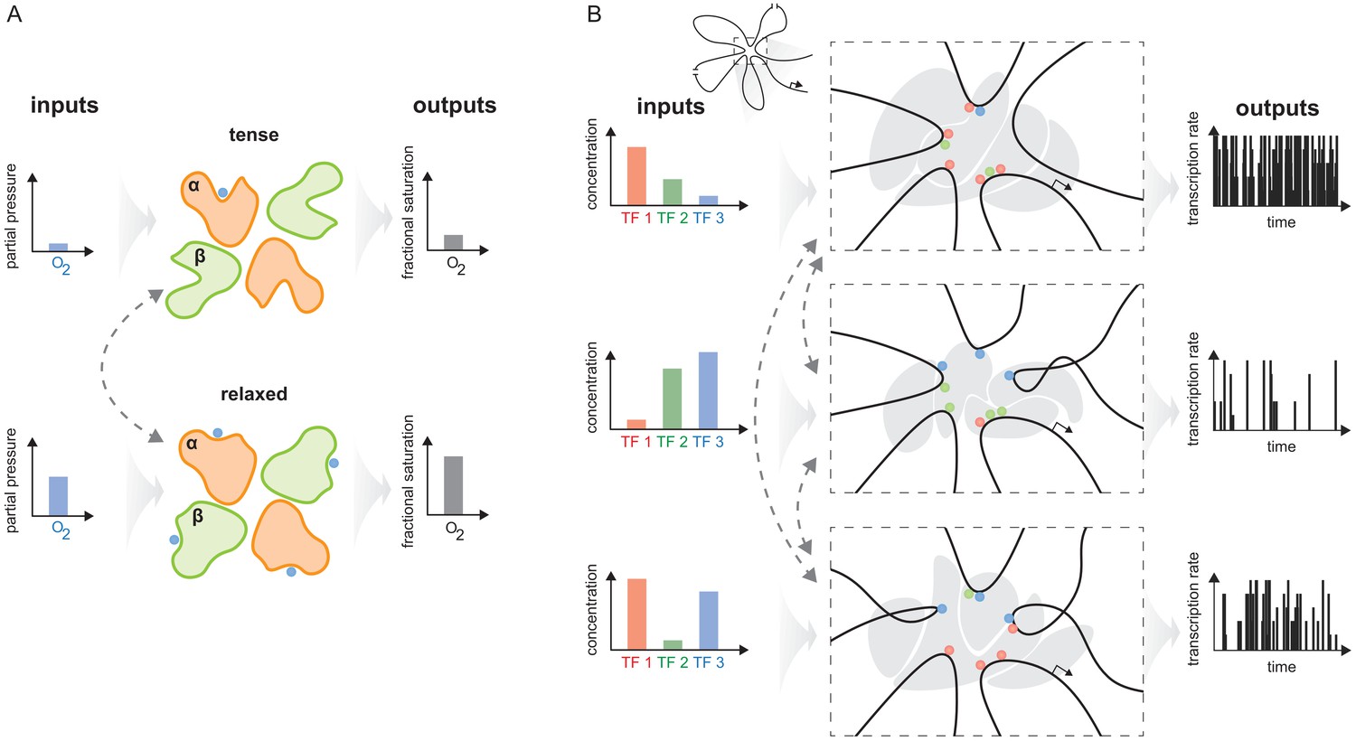
The haemoglobin analogy in gene regulation.
(A) The two conformations of haemoglobin are each adapted to one of the two input-output functions which haemoglobin integrates to solve the oxygen transport problem. These conformations dynamically interchange in the ensemble (grey dashed arrows). (B) The gene regulatory machinery couples input patterns of transcription factors (TFs) (left) to output patterns of stochastic expression of mRNA splice isoforms (right, showing bursting patterns of one isoform). Our results suggest that a sufficiently complex conformational ensemble, built out of chromatin, TFs, co-regulators and phase-separated condensates (centre, grey shapes in three distinct conformations), could integrate these functions at a single gene in an analogous way to haemoglobin. Chromatin is represented by the thick black curve, whose looped arrangement around the promoter is shown schematically (top).
Scheme 1
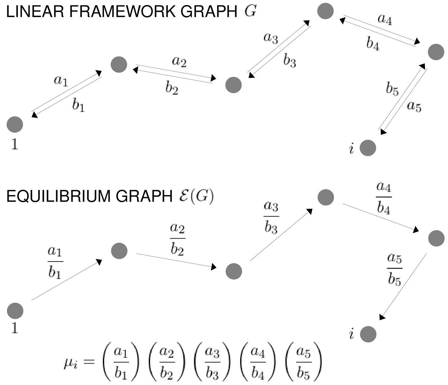
Graphs and equilibrium calculations.
At top, a path of reversible edges in a linear framework graph, , from the reference vertex, 1, to a vertex , with the edge labels shown. Below is the same path in the corresponding equilibrium graph, , showing the equilibrium labels, as given by Equation 31. The formula for the quantity , as specified in Equation 30, is shown at bottom. For μ to be well defined, must satisfy detailed balance (Equation 29) or, equivalently, the cycle condition (Equation 32) must hold in . Equilibrium probabilities are calculated from μ using Equation 33.
Scheme 2
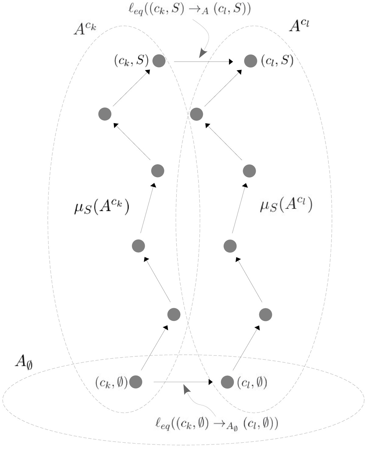
Illustration of Equation 38.
A hypothetical allostery graph shows how the label for the edge at the top, which links the vertical subgraphs at conformations ck and cl at the binding subset , can be calculated from the quantities and and the edge label at the bottom. The quantities come from paths to the vertices in question from the respective reference vertices in the vertical subgraphs, as specified in Equation 30 and Scheme 1. The edge label at the bottom comes from the horizontal subgraph of empty conformations, . The vertical subgraphs and have the same structure and the paths are shown as the same in each subgraph, but they could be arbitrary paths because of the cycle condition at thermodynamic equilibrium (Equation 32). Once appropriate directions are taken, the two paths and the edges at the top and bottom constitute a large cycle in the allostery graph and Equation 38 is simply a rewriting of Equation 32 applied to this cycle.
Scheme 3

Coarse graining and effective association constants.
At top left is an example allostery graph, with binding of a single ligand to sites for conformations. Vertices indicate a bound site with a solid black dot and an unbound site with a black dash and binding subsets are colour coded: both sites unbound, black; only site 1 bound, magenta; only site 2 bound, cyan; both sites bound, blue. Some vertices are annotated and some edge labels are shown, with denoting ligand concentration. Note that the allostery graph has been oriented with its reference vertex at the top, in contrast to the graphs in the main text figures, in order to accommodate the formulas. Example calculations of based on Equation 30 are shown for the vertical subgraph . At bottom is the horizontal subgraph along with the calculation of its steady-state probability distribution in terms of the equilibrium labels, . and the quantities . At top right is the coarse-grained allostery graph, , with vertices colour coded as for the binding subsets of the allostery graph. Equation 48 for the effective association constants is illustrated below .
Additional files
Download links
A two-part list of links to download the article, or parts of the article, in various formats.
Downloads (link to download the article as PDF)
Open citations (links to open the citations from this article in various online reference manager services)
Cite this article (links to download the citations from this article in formats compatible with various reference manager tools)
Allosteric conformational ensembles have unlimited capacity for integrating information
eLife 10:e65498.
https://doi.org/10.7554/eLife.65498


