Mice in a labyrinth show rapid learning, sudden insight, and efficient exploration
- Division of Biology and Biological Engineering, California Institute of Technology, United States
- Division of Engineering and Applied Science, California Institute of Technology, United States
Figures
Figure 1 with 3 supplements
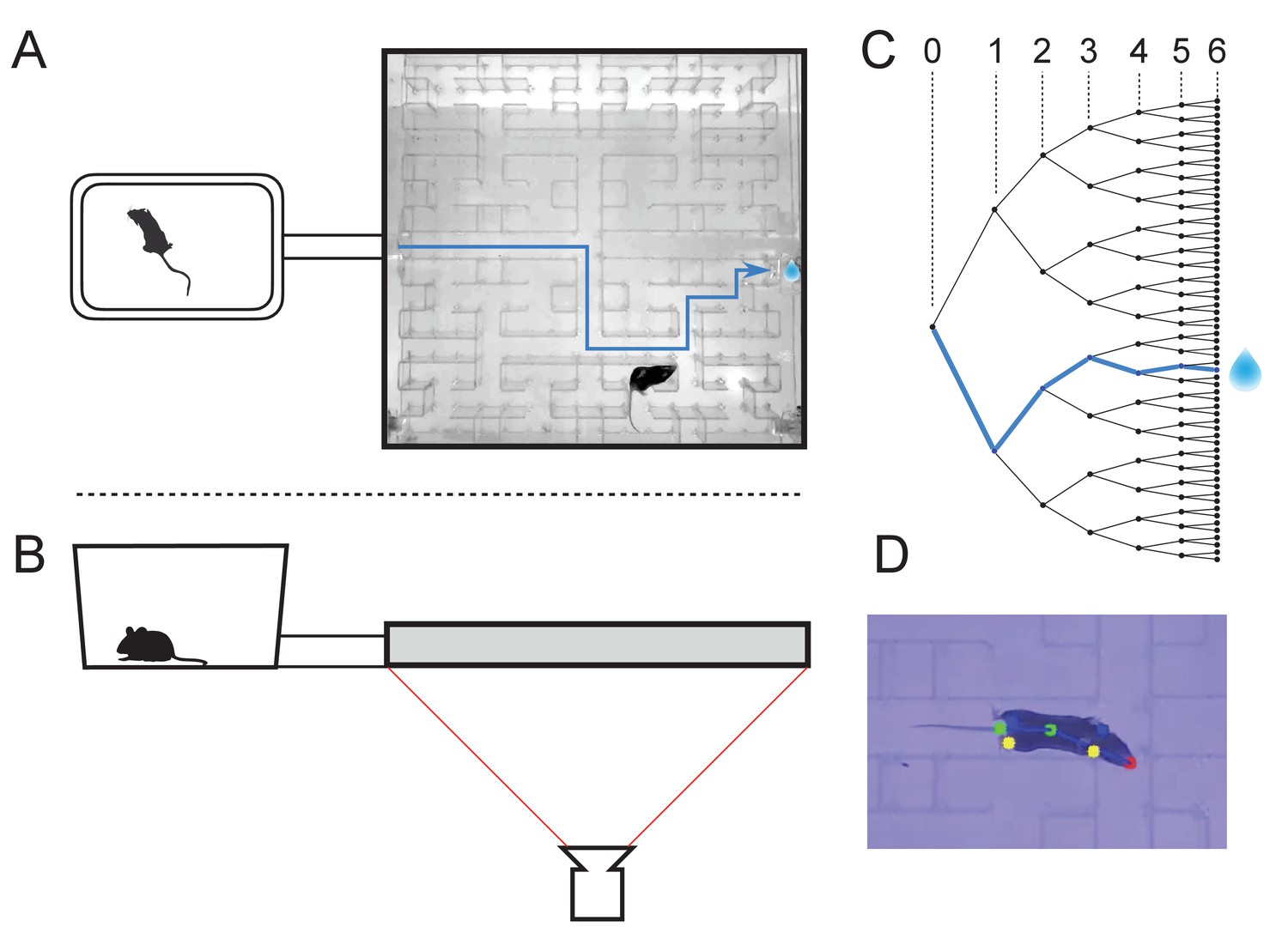
The maze environment.
Top (A) and side (B) views of a home cage, connected via an entry tunnel to an enclosed labyrinth. The animal’s actions in the maze are recorded via video from below using infrared illumination. (C) The maze is structured as a binary tree with 63 branch points (in levels numbered 0,…,5) and 64 end nodes. One end node has a water port that dispenses a drop when it gets poked. Blue line in A and C: path from maze entry to water port. (D) A mouse considering the options at the maze’s central intersection. Colored keypoints are tracked by DeepLabCut: nose, mid body, tail base, four feet.
Figure 1—figure supplement 1
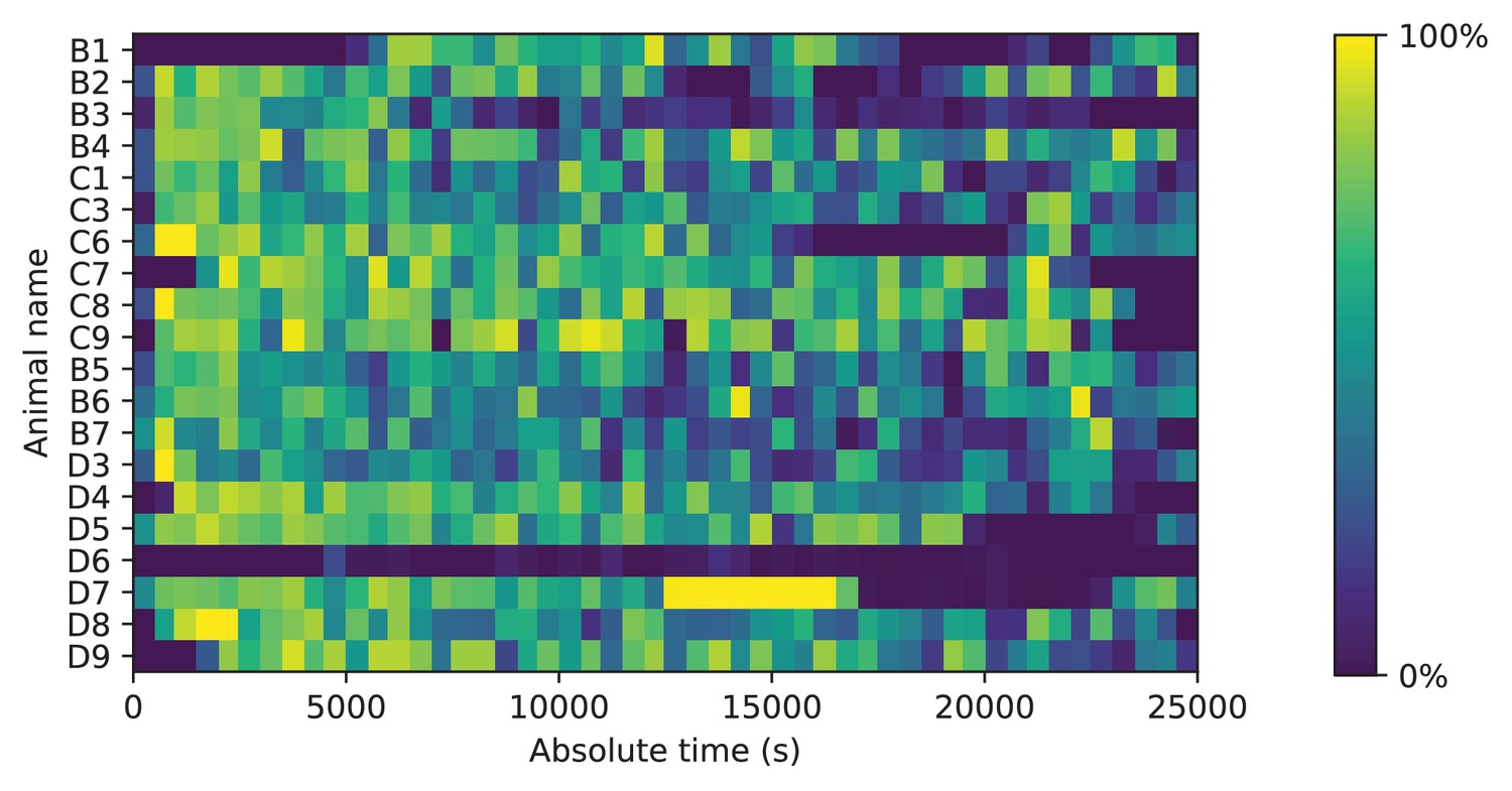
Occupancy of the maze.
Fraction of time spent in the maze. Mice could move freely between the home cage and the maze. For each animal (vertical), the fraction of time in the maze (color scale) is plotted as a function of time since start of the experiment. Time bins are 500 s. Note that mouse D6 hardly entered the maze; it never progressed beyond the first junction. This animal was excluded from all subsequent analysis steps.
Figure 1—figure supplement 2
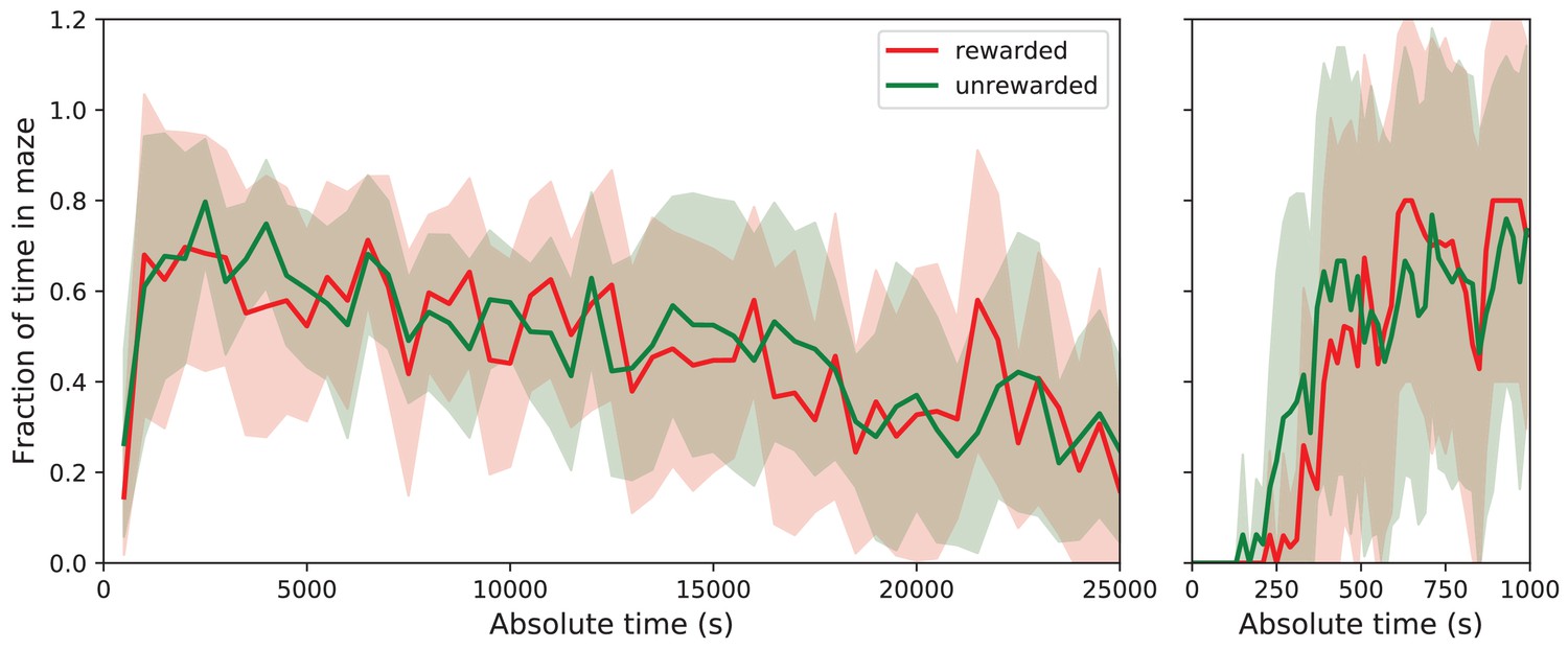
Fraction of time in maze by group.
Average fraction of time spent in the maze by group. This shows the average fraction of time in the maze as Mean ± SD over the population of 10 rewarded and nine unrewarded animals. Right: expanded axis for early times. The tunnel to the maze opens at time 0. Rewarded and unrewarded animals used the maze in remarkably similar ways. Exploration of the maze began around 250 s after tunnel opening. Within the next 250 s, the maze occupancy rose quickly to ~70%, then declined gradually over 7 h to ~30%.
Figure 1—figure supplement 3
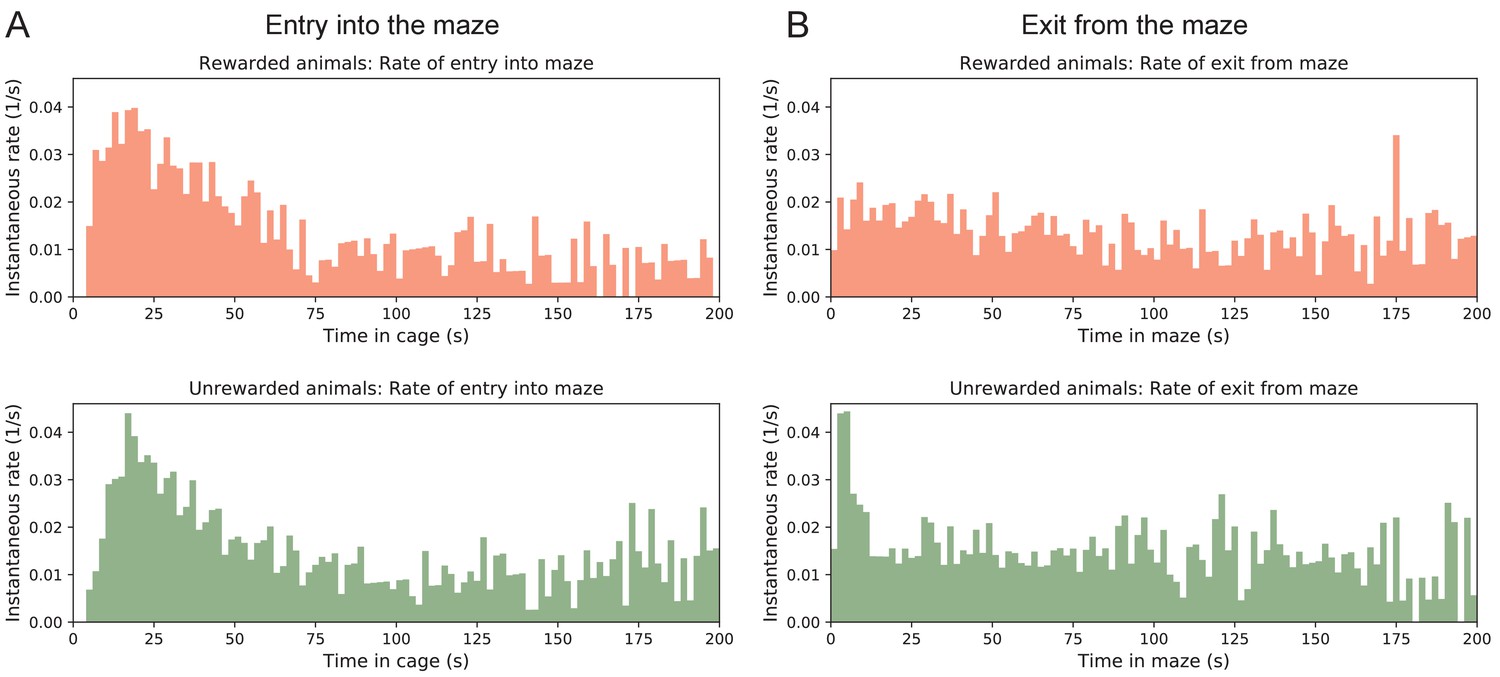
Transitions between cage and maze.
Rates of transition between cage and maze. (A) The instantaneous probability per unit time of entering the maze after having spent time in the cage. Note this rate is highest immediately upon entering the cage, then declines by a large factor. (B) The instantaneous probability per unit time of exiting the maze after having spent time in the maze.
Figure 2 with 1 supplement
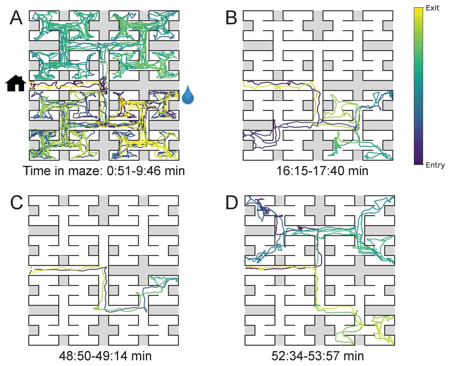
Sample trajectories during adaptation to the maze.
Four sample bouts from one mouse (B3) into the maze at various times during the experiment (time markings at bottom). The trajectory of the animal’s nose is shown; time is encoded by the color of the trace. The entrance from the home cage and the water port are indicated in panel A.
Figure 2—figure supplement 1
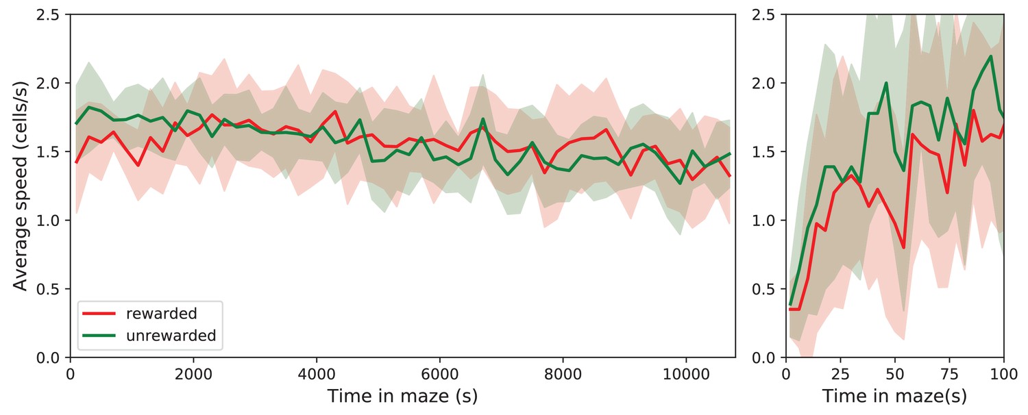
Speed of locomotion.
The speed of locomotion in the maze is approximately constant. Left: Speed plotted as Mean ± SD over the population of rewarded and unrewarded animals. Right: expanded axis for early times. To assess the speed of locomotion, we divided the maze into square cells as wide as the corridors and tracked how the nose of the animal moved through those cells. Then the speed was measured in number of cells traversed per unit time. Note that the speed is very similar across animals, ~1.56 cells/s = 5.94 cm/s on average. It rises quickly over the first 50 s in the maze, then varies only little over the 7 h of the experiment.
Figure 3 with 1 supplement
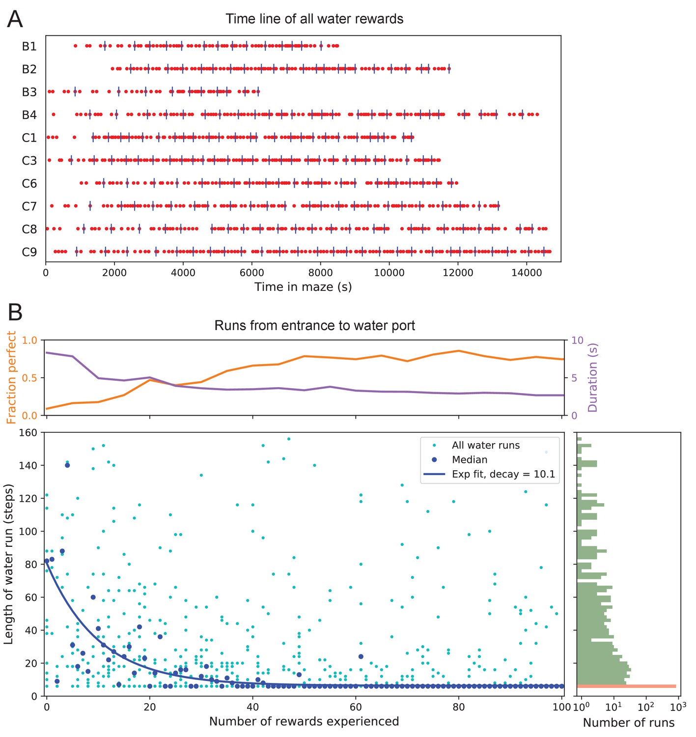
Few-shot learning of path to water.
(A) Time line of all water rewards collected by 10 water-deprived mice (red dots, every fifth reward has a blue tick mark). (B) The length of runs from the entrance to the water port, measured in steps between nodes, and plotted against the number of rewards experienced. Main panel: All individual runs (cyan dots) and median over 10 mice (blue circles). Exponential fit decays by over 10.1 rewards. Right panel: Histogram of the run length, note log axis. Red: perfect runs with the minimum length 6; green: longer runs. Top panel: The fraction of perfect runs (length 6) plotted against the number of rewards experienced, along with the median duration of those perfect runs.
Figure 3—figure supplement 1
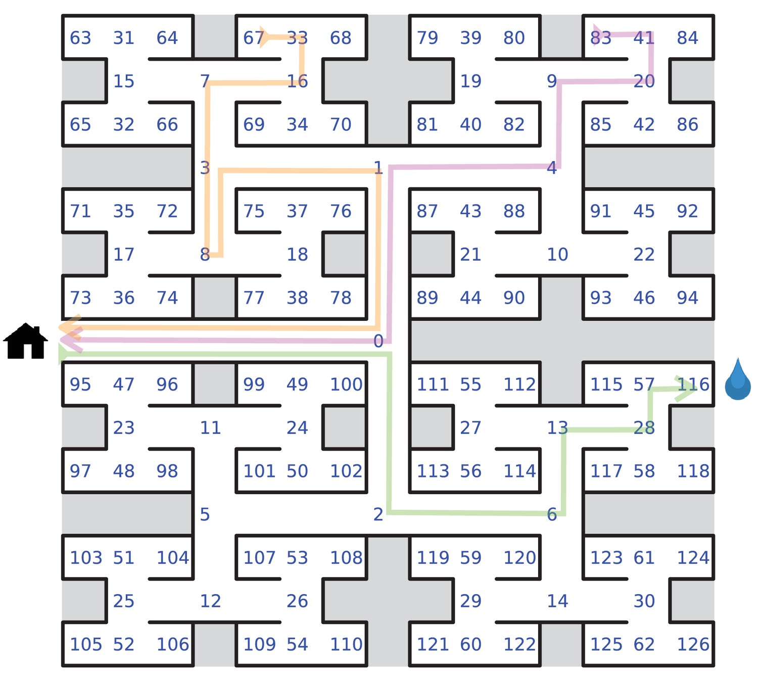
Definition of node trajectories.
Definition of node trajectories. A numbering scheme for all 127 nodes of the maze. Green: a direct path from the entrance to the water port (‘water run’) with the node sequence , involving six decisions. Magenta: a direct path from end node 83 to the exit (‘home run’). Orange: a path from end node 67 to the exit that includes a reversal. Here the home run starts only from node 8, namely .
Figure 4 with 2 supplements
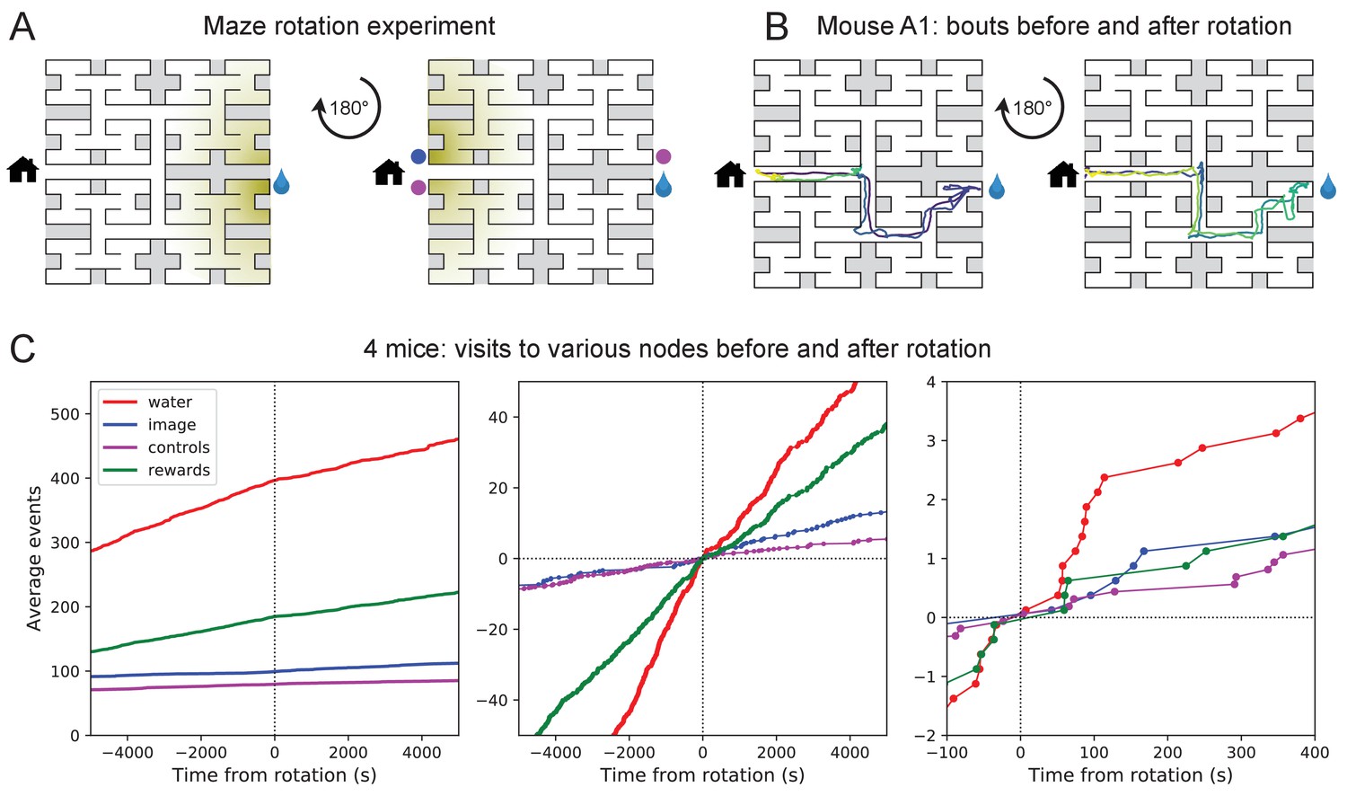
Navigation is robust to rotation of the maze.
(A) Logic of the experiment: The animal may have deposited an odorant in the maze (shading) that is centered on the water port. After 180 degree rotation of the maze, that gradient would lead to the image of the water port (blue dot). We also measure how often the mouse goes to two control nodes (magenta dots) that are related by symmetry. (B) Trajectory of mouse ‘A1’ in the bouts immediately before and after maze rotation. Time coded by color from dark to light as in Figure 2. (C) Left: Cumulative number of rewards as well as visits to the water port, the image of the water port, and the control nodes. All events are plotted vs time before and after the maze rotation. Average over four animals. Middle and right: Same data with the counts centered on zero and zoomed in for better resolution.
Figure 4—figure supplement 1
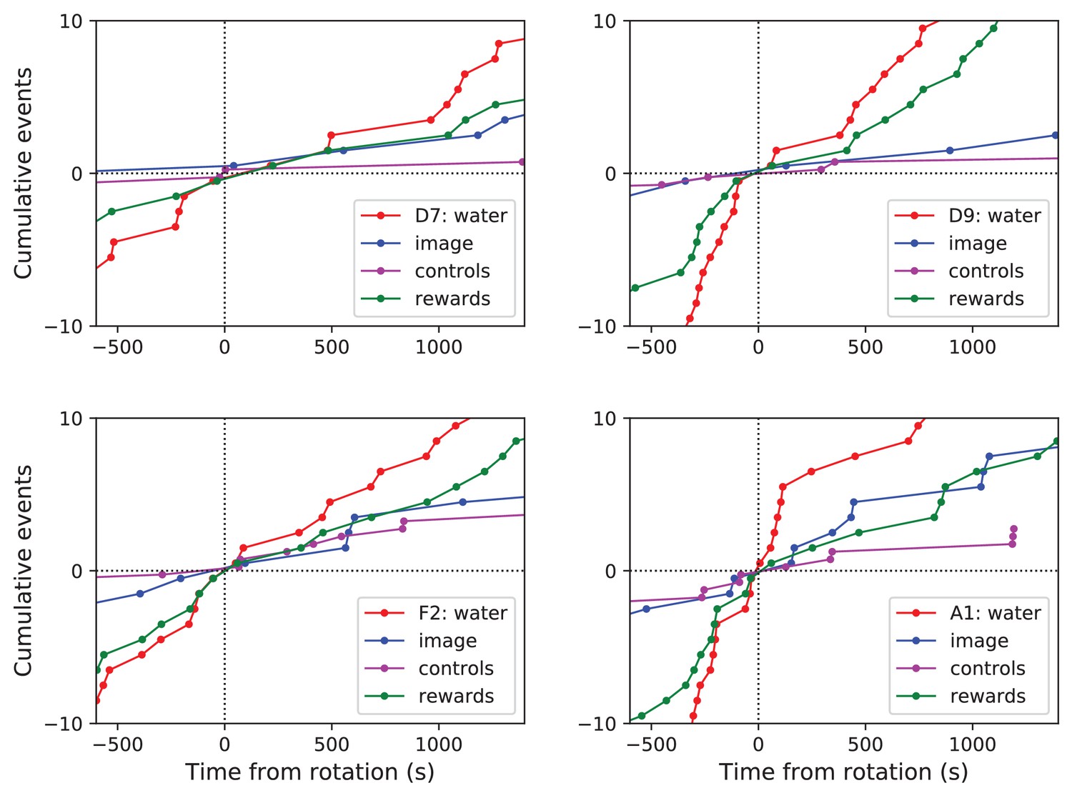
Navigation before and after maze rotation for each animal.
Navigation before and after maze rotation. Cumulative number of rewards, visits to the water port, the image of the water port, and the control nodes, plotted vs time before and after the maze rotation. Display as in Figure 4C, but split for each of four animals.
Figure 4—figure supplement 2
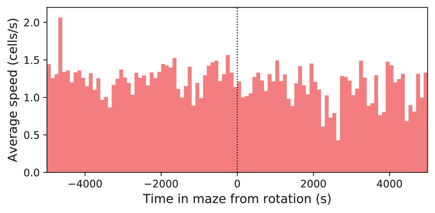
Speed before and after maze rotation.
Speed of the mouse vs time in the maze. Average over four animals. Time is plotted relative to the maze rotation.
Figure 5 with 1 supplement
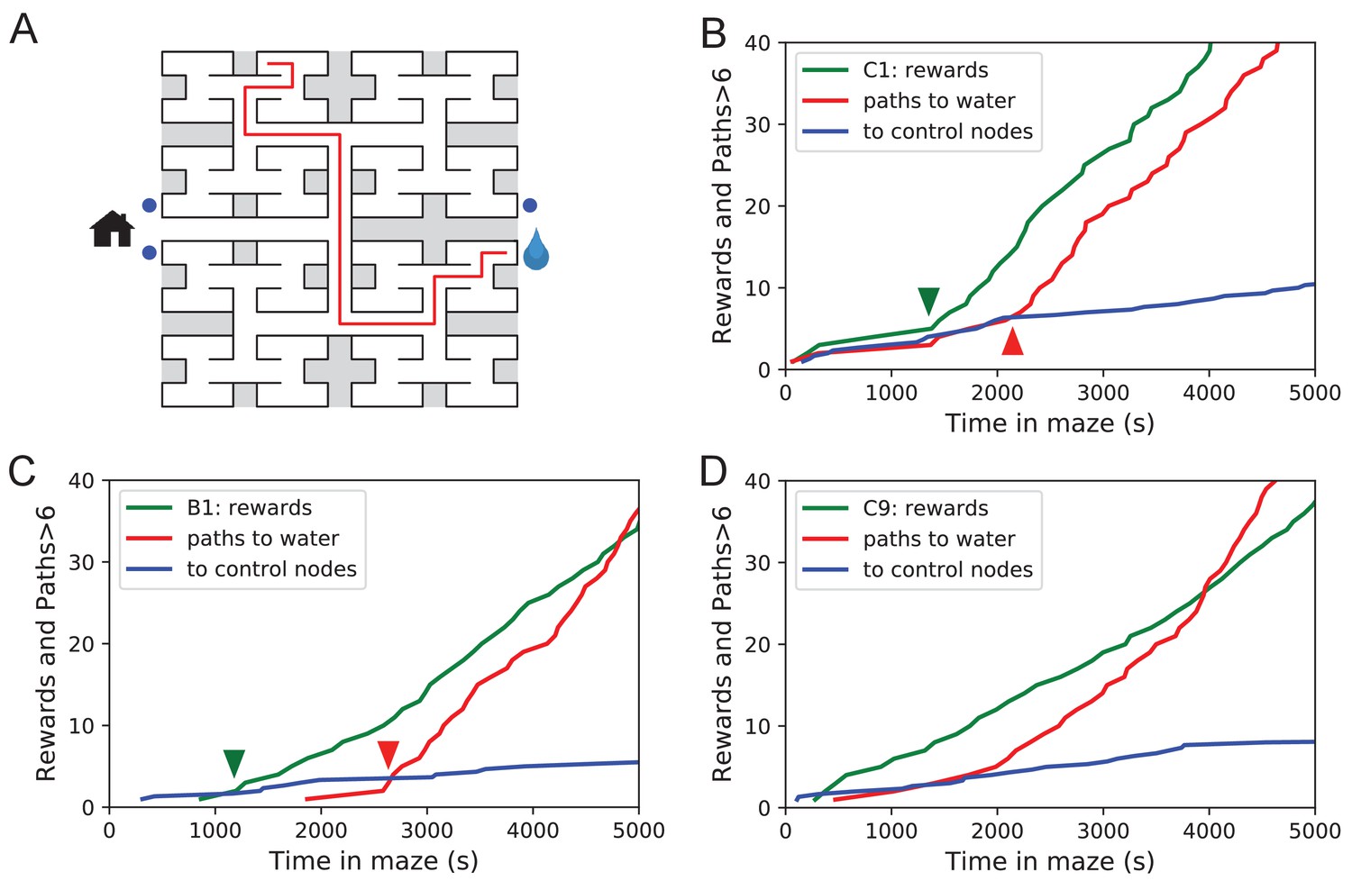
Sudden changes in behavior.
(A) An example of a long uninterrupted path through 11 junctions to the water port (drop icon). Blue circles mark control nodes related by symmetry to the water port to assess the frequency of long paths occurring by chance. (B) For one animal (named C1) the cumulative number of rewards (green); of long paths (>6 junctions) to the water port (red); and of similar paths to the three control nodes (blue, divided by 3). All are plotted against the time spent in the maze. Arrowheads indicate the time of sudden changes, obtained from fitting a step function to the rates. (C) Same as B for animal B1. (D) Same as B for animal C9, an example of more continuous learning.
-
Figure 5—source data 1
Statistics of sudden changes in behavior.
Statistics of sudden changes in behavior. Summary of the steps in the rate of long paths to water detected in 5 of the 10 rewarded animals. Mean and standard deviation of the step time are derived from maximum likelihood fits of a step model to the data.
- https://cdn.elifesciences.org/articles/66175/elife-66175-fig5-data1-v2.pdf
Figure 5—figure supplement 1
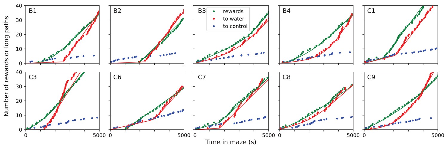
Long direct paths for all animals.
Sudden changes in behavior for all rewarded animals. For each of the 10 water-deprived animals this shows the cumulative rate of rewards, of long direct paths (>6 steps) to the water port, and of similar paths to three control nodes. Display as in Figure 5; panels B-D of that figure are included again here. Dots are data, lines are fits using a four-parameter sigmoid function for the rate of occurrence of the events.
Figure 6
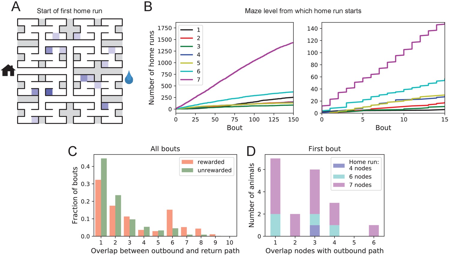
Homing succeeds on first attempt.
(A) Locations in the maze where the 19 animals started their first return to the exit (home run). Some locations were used by two or three animals (darker color). (B) Left: The cumulative number of home runs from different levels in the maze, summed over all animals, and plotted against the bout number. Level 1 = first T-junction, level 7 = end nodes. Right: Zoom of (Left) into early bouts. (C) Overlap between the outbound and the home path. Histogram of the overlap for all bouts of all animals. (D) Same analysis for just the first bout of each animal. The length of the home run is color-coded as in panel B.
Figure 7
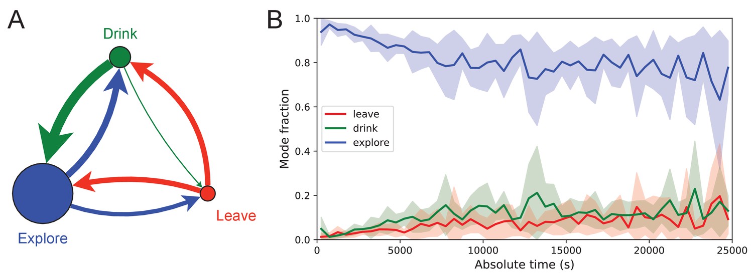
Exploration is a dominant and persistent mode of behavior.
(A) Ethogram for rewarded animals. Area of the circle reflects the fraction of time spent in each behavioral mode averaged over animals and duration of the experiment. Width of the arrow reflects the probability of transitioning to another mode. ‘Drink’ involves travel to the water port and time spent there. Transitions from ‘Leave’ represent what the animal does at the start of the next bout into the maze. (B) The fraction of time spent in each mode as a function of absolute time throughout the night. Mean ± SD across the 10 rewarded animals.
-
Figure 7—source data 1
Three modes of behavior.
(A) The fraction of time mice spent in each of the three modes while in the maze. Mean ± SD for 10 rewarded and nine unrewarded animals. (B) Probability of transitioning from the mode on the left to the mode at the top. Transitions from ‘leave’ represent what the animal does at the start of the next bout into the maze.
- https://cdn.elifesciences.org/articles/66175/elife-66175-fig7-data1-v2.pdf
Figure 8 with 1 supplement
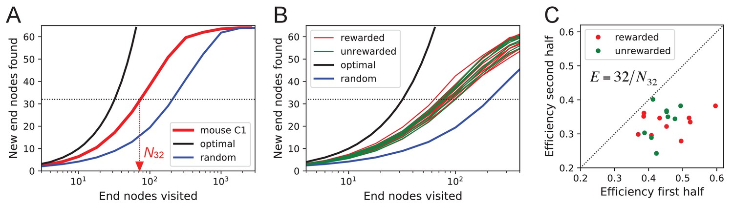
Exploration covers the maze efficiently.
(A) The number of distinct end nodes encountered as a function of the number of end nodes visited for: mouse C1 (red); the optimal explorer agent (black); an unbiased random walk (blue). Arrowhead: the value by which mouse C1 discovered half of the end nodes. (B) An expanded section of the graph in A including curves from 10 rewarded (red) and nine unrewarded (green) animals. The efficiency of exploration, defined as , is (SD) for rewarded and (SD) for unrewarded mice. (C) The efficiency of exploration for the same animals, comparing the values in the first and second halves of the time in the maze. The decline is a factor of (SD) for rewarded and (SD) for unrewarded mice.
Figure 8—figure supplement 1
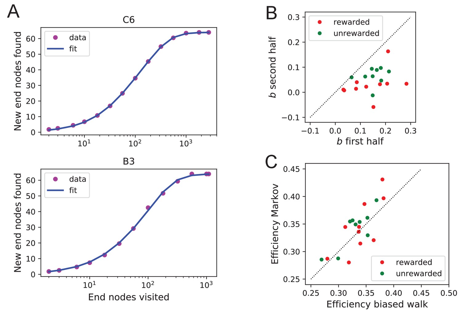
Efficiency of exploration.
Functional fits to measure exploration efficiency (A) Fitting Equation 12 to the data from the mouse’s exploration. Animals with best fit (top) and worst fit (bottom). The relative uncertainty in the two fit parameters and was only (mean ± SD across animals). (B) The fit parameter for all animals, comparing the first to the second half of the night. (C) The efficiency (Equation 1) predicted from two models of the mouse’s trajectory: The 4-bias random walk (Figure 11D) and the optimal Markov chain (Figure 11C).
Figure 9
Turning biases favor exploration.
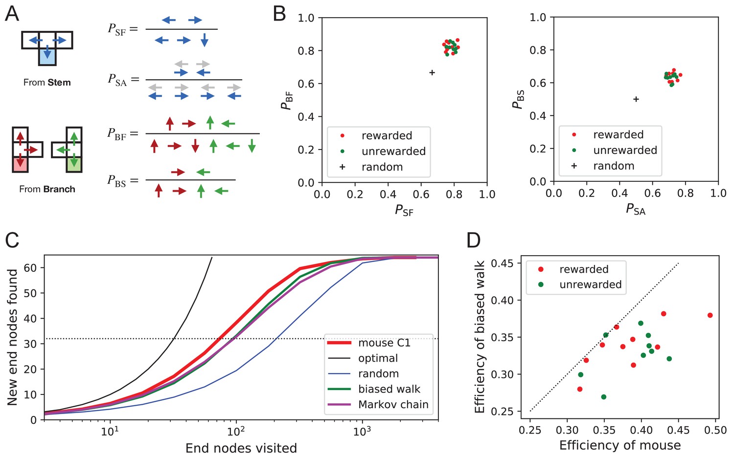
(A) Definition of four turning biases at a T-junction based on the ratios of actions taken. Top: An animal arriving from the stem of the T (shaded) may either reverse or turn left or right. is the probability that it will move forward rather than reversing. Given that it moves forward, is the probability that it will take an alternating turn from the preceding one (gray), that is left-right or right-left. Bottom: An animal arriving from the bar of the T may either reverse or go straight, or turn into the stem of the T. is the probability that it will move forward through the junction rather than reversing. Given that it moves forward, is the probability that it turns into the stem. (B) Scatter graph of the biases and (left) and and (right). Every dot represents a mouse. Cross: values for an unbiased random walk. (C) Exploration curve of new end nodes discovered vs end nodes visited, displayed as in Figure 8A, including results from a biased random walk with the four turning biases derived from the same mouse, as well as a more elaborate Markov-chain model (see Figure 11C). (D) Efficiency of exploration (Equation 1) in 19 mice compared to the efficiency of the corresponding biased random walk.
-
Figure 9—source data 1
Bias statistics.
Statistics of the four turning biases. Mean and standard deviation of the 4 biases of Figure 9A–B across animals in the rewarded and unrewarded groups.
- https://cdn.elifesciences.org/articles/66175/elife-66175-fig9-data1-v2.pdf
Figure 10
Preference for certain end nodes during exploration.
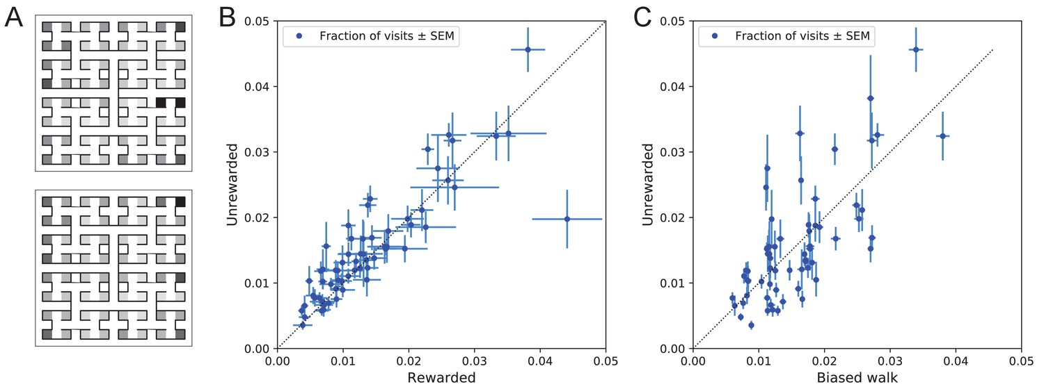
(A) The number of visits to different end nodes encoded by a gray scale. Top: rewarded, bottom: unrewarded animals. Gray scale spans a factor of 12 (top) or 13 (bottom). (B) The fraction of visits to each end node, comparing the rewarded vs unrewarded group of animals. Each data point is for one end node, the error bar is the SEM across animals in the group. The outlier on the bottom right is the neighbor of the water port, a frequently visited end node among rewarded animals. The water port is off scale and not shown. (C) As in panel B but comparing the unrewarded animals to their simulated 4-bias random walks. These biases explain 51% of the variance in the observed preference for end nodes.
Figure 11 with 1 supplement
Recent history constrains the mouse’s decisions.
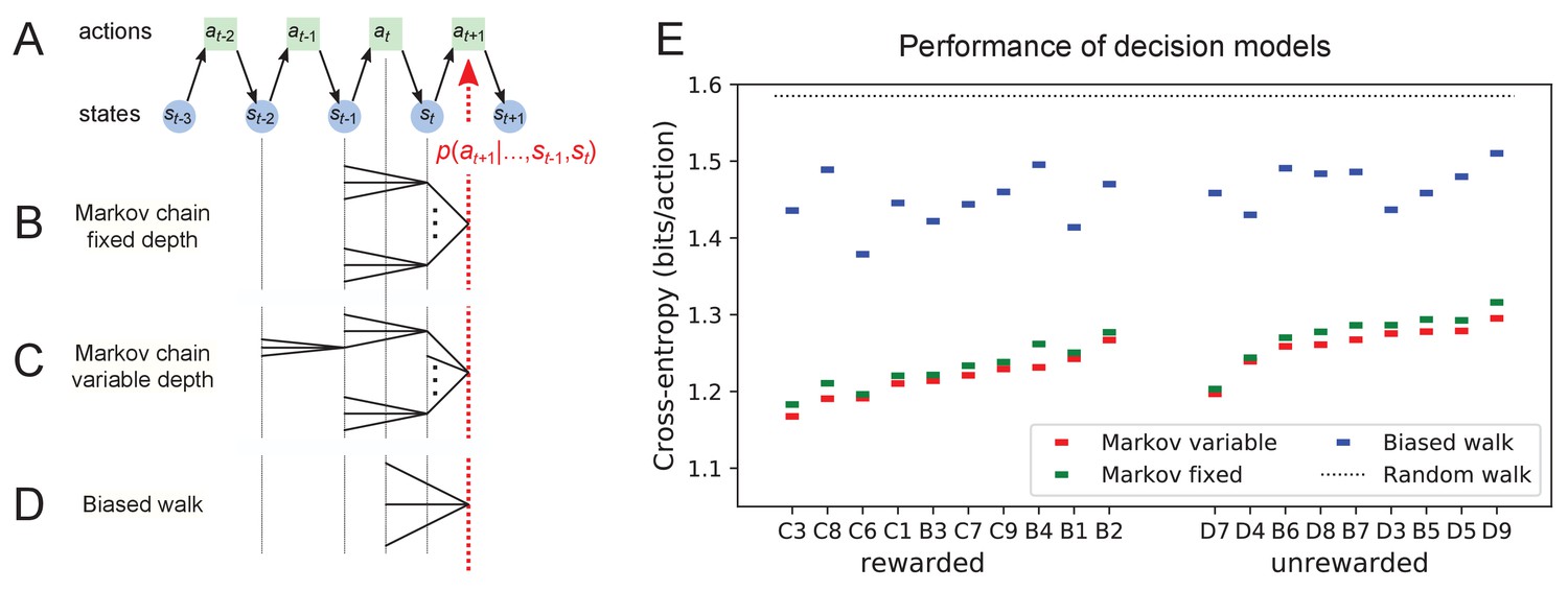
(A) The mouse’s trajectory through the maze produces a sequence of states . From each state, up to three possible actions lead to the next state (end nodes allow only one action). We want to predict the animal’s next action, , based on the prior history of states or actions. (B–D) Three possible models to make such a prediction. (B) A fixed-depth Markov chain where the probability of the next action depends only on the current state and the preceding state . The branches of the tree represent all possible histories . (C) A variable-depth Markov chain where only certain branches of the tree of histories contribute to the action probability. Here one history contains only the current state, some others reach back three steps. (D) A biased random walk model, as defined in Figure 9, in which the probability of the next action depends only on the preceding action, not on the state. (E) Performance of the models in (B,C,D) when predicting the decisions of the animal at T-junctions. In each case we show the cross-entropy between the predicted action probability and the real actions of the animal (lower values indicate better prediction, perfect prediction would produce zero). Dotted line represents an unbiased random walk with 1/3 probability of each action.
Figure 11—figure supplement 1
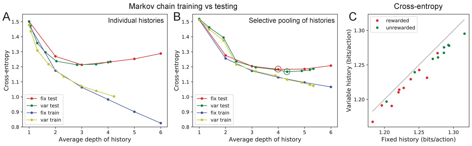
Markov model fits.
Fitting Markov models of behavior. (A) Results of fitting the node sequence of a single animal (C3) with Markov models having a fixed depth (‘fix’) or variable depth (‘var’). The cross-entropy of the model’s prediction is plotted as a function of the average depth of history. In both cases we compare the results obtained on the training data (‘train’) vs those on separate testing data (‘test’). Note that at larger depth the ‘test’ and ‘train’ estimates diverge, a sign of over-fitting the limited data available. (B) As in (A) but to combat the data limitation we pooled the counts obtained at all nodes that were equivalent under the symmetry of the maze (see Materials and methods). Note considerably less divergence between ‘train’ and ‘test’ results, and a slightly lower cross-entropy during ‘test’ than in (A). (C) The minimal cross-entropy (circles in (B)) produced by variable vs fixed history models for each of the 19 animals. Note the variable history model always produces a better fit to the behavior.
Additional files
Download links
A two-part list of links to download the article, or parts of the article, in various formats.
Downloads (link to download the article as PDF)
Open citations (links to open the citations from this article in various online reference manager services)
Cite this article (links to download the citations from this article in formats compatible with various reference manager tools)
Mice in a labyrinth show rapid learning, sudden insight, and efficient exploration
eLife 10:e66175.
https://doi.org/10.7554/eLife.66175


