Host-associated microbe PCR (hamPCR) enables convenient measurement of both microbial load and community composition
- Department of Molecular Biology, Max Planck Institute for Developmental Biology, Germany
- Department of Evolutionary Biology, Max Planck Institute for Developmental Biology, Germany
- ZMBP-General Genetics, University of Tübingen, Germany
Figures
Figure 1 with 1 supplement
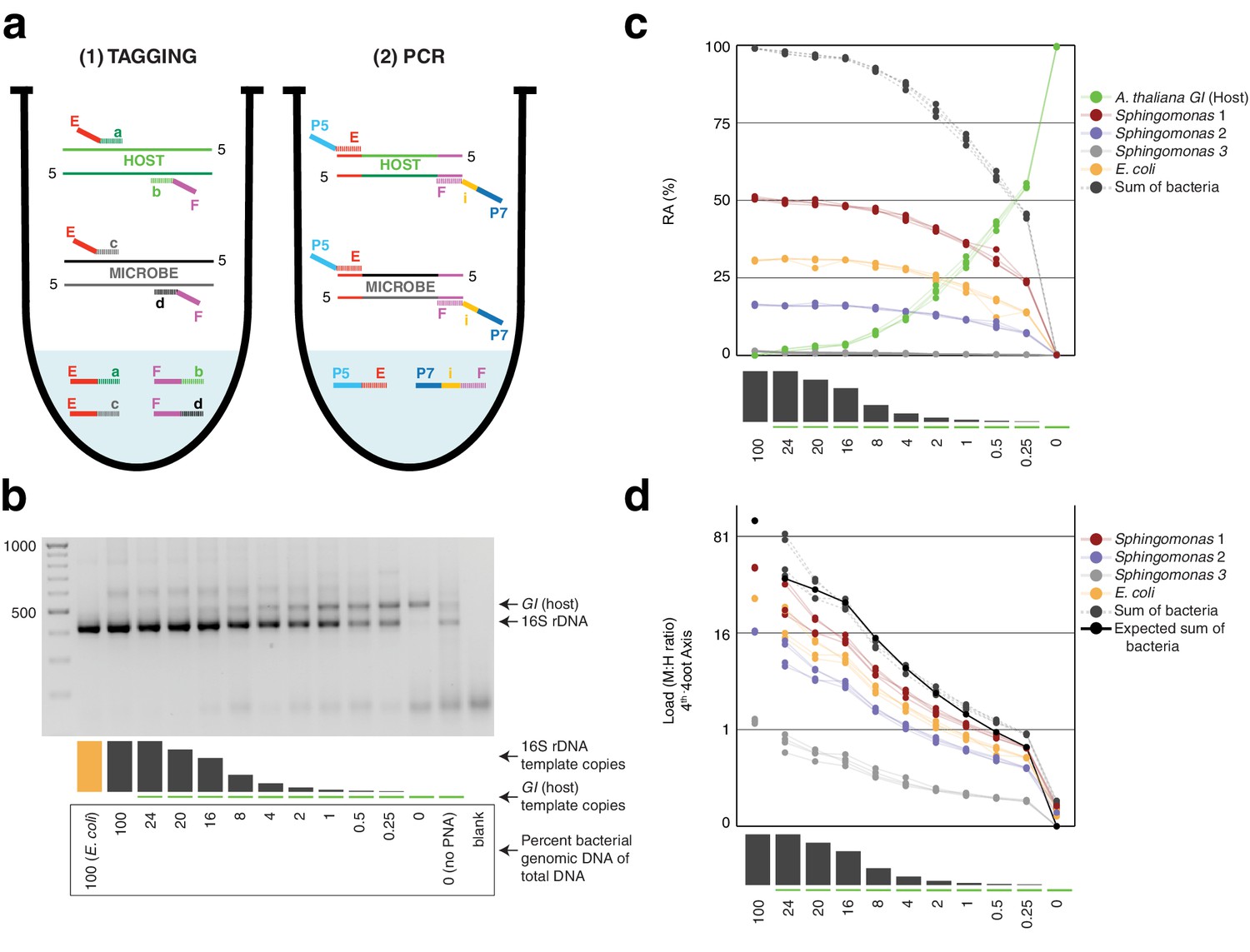
Synthetic samples demonstrate technical reproducibility.
(a) Schematic showing the two steps of hamPCR. The HM-tagging reaction (left) shows two primer pairs: one for the host (E-a and F-b) and one for microbes (E-c and F-d). Each primer pair adds the same universal overhangs E and F. The PCR reaction (right) shows a single primer pair (P7-E and P5-i-F) that can amplify all tagged products. (b) Representative 2% agarose gel of hamPCR products from the synthetic titration panel, showing a V4 16S rDNA amplicon at ~420 bp and an A. thaliana GI amplicon at 502 bp. The barplot underneath shows the predicted number of original GI and 16S rDNA template copies. Numbers boxed below the barplot indicate the percent bacterial genomic DNA of total DNA. (c) Relative abundance of the host and microbial ASVs in the synthetic titration panel, as determined by amplicon counting. Pure E. coli, pure A. thaliana without PNAs, and blanks were excluded. (d) Data in (c) converted to microbial load by dividing by host abundance, with a fourth-root transformed y-axis to better visualize lower abundances.
Figure 1—figure supplement 1

Gel images from synthetic titration panel.
(a) hamPCR using the 502 bp A. thaliana GI amplicon and the ~420 bp V4 16S rDNA amplicon (515F - 799R) was performed with the samples of the synthetic titration panel, and 5 μL of the PCR product from each sample was analyzed on a 2% agarose gel. This was done across four replicates each prepared with an independent PCR master mix. Due to a technical failure in replicate 1, the sample with 0.25% bacteria did not yield any product and was redone in a separate reaction. (b) The same as (a), except using the ~587 bp V3V4 16S rDNA amplicon (341F - 799R). (c) The same as (a) and (b), except using the 466 bp A. thaliana GI amplicon and the ~540 bp V5V6V7 16S rDNA amplicon (799F - 1192R). This 16S rDNA primer set also amplifies a ~770 bp region of mitochondria, producing a final amplicon of about 900 bp. In practice, the mitochondrial band is usually removed by gel extraction of the desired amplicons prior to sequencing.
Figure 2 with 2 supplements
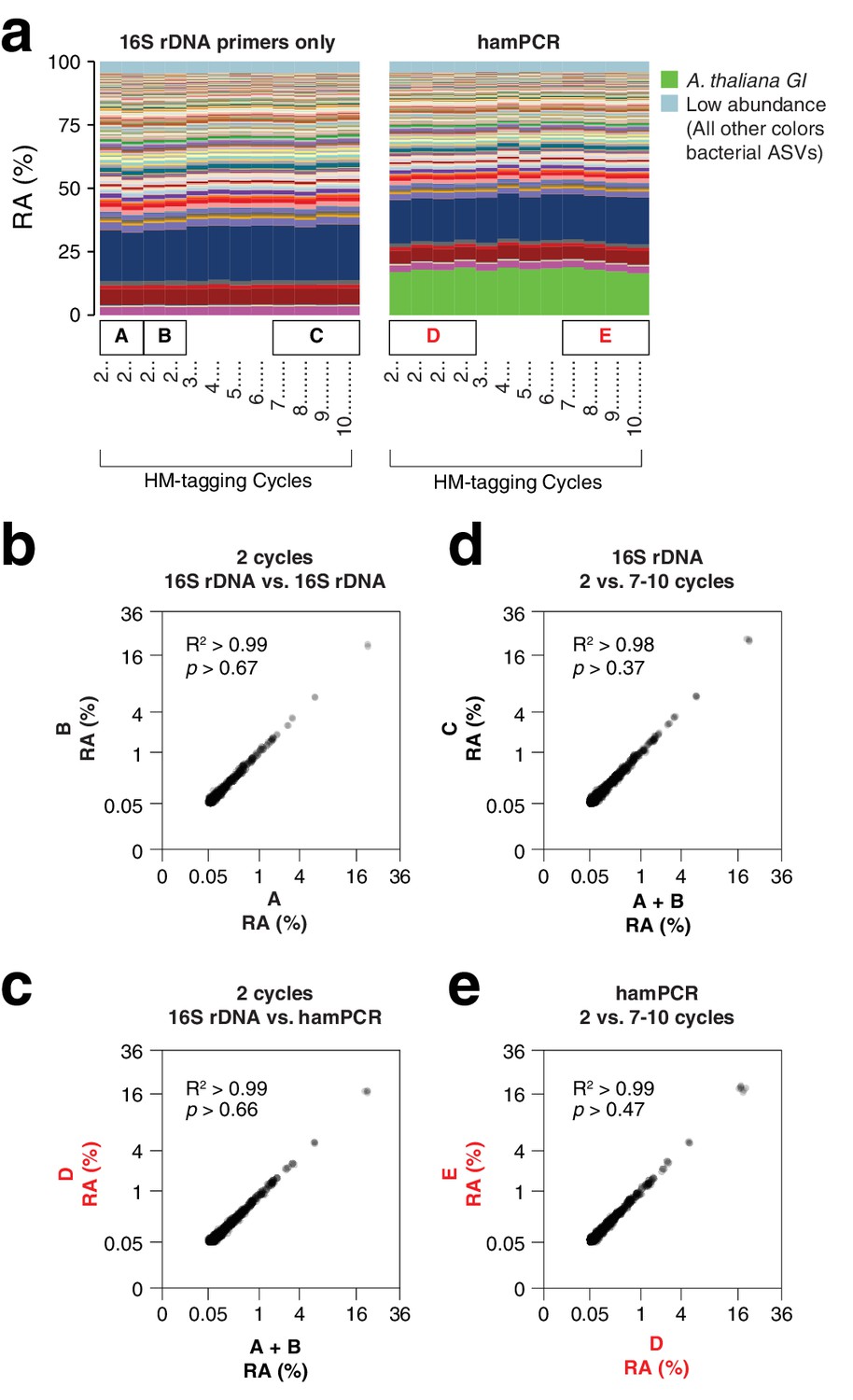
hamPCR is robust and does not distort a complex microbial community.
(a) DNA extracted from wild A. thaliana phyllospheres was used as a template for both V4 16S rDNA PCR (left, 515F and 799R) and hamPCR (right, V4 16S rDNA and GI 502 bp primers). Four replicates were produced with two cycles of the HM-tagging reaction and 30 cycles of PCR, and additional replicates with 3 to 10 HM-tagging cycles paired with 29 to 22 PCR cycles (for a constant total of 32 cycles). The stacked columns show the relative abundances of major ASVs. Boxed upper case letters demarcate groups of samples compared below. (b) Correlation of fourth-root transformed ASV abundances for the 16S rDNA samples above panel (a) box [A] to the 16S rDNA samples above box [B]. Only ASVs with a minimum relative abundance of 0.05% were compared. R2, coefficient of determination. p-value from Kolmogorov-Smirnov test. (c) Same as (b), but for the four 16S rDNA samples above box [A] and [B] compared to the four hamPCR samples above box [D]. For hamPCR, the A. thaliana GI ASV was removed and the bacterial ASVs were rescaled to 100% prior to the comparison. (d) Same as (b) and (c), but for the four 16S rDNA samples above box [A] and [B] compared to the 16S rDNA samples above box [C]. (e) Same as (b), (c), and (d), but for the four hamPCR samples above box [D] compared to the four hamPCR samples above box [E].
Figure 2—figure supplement 1
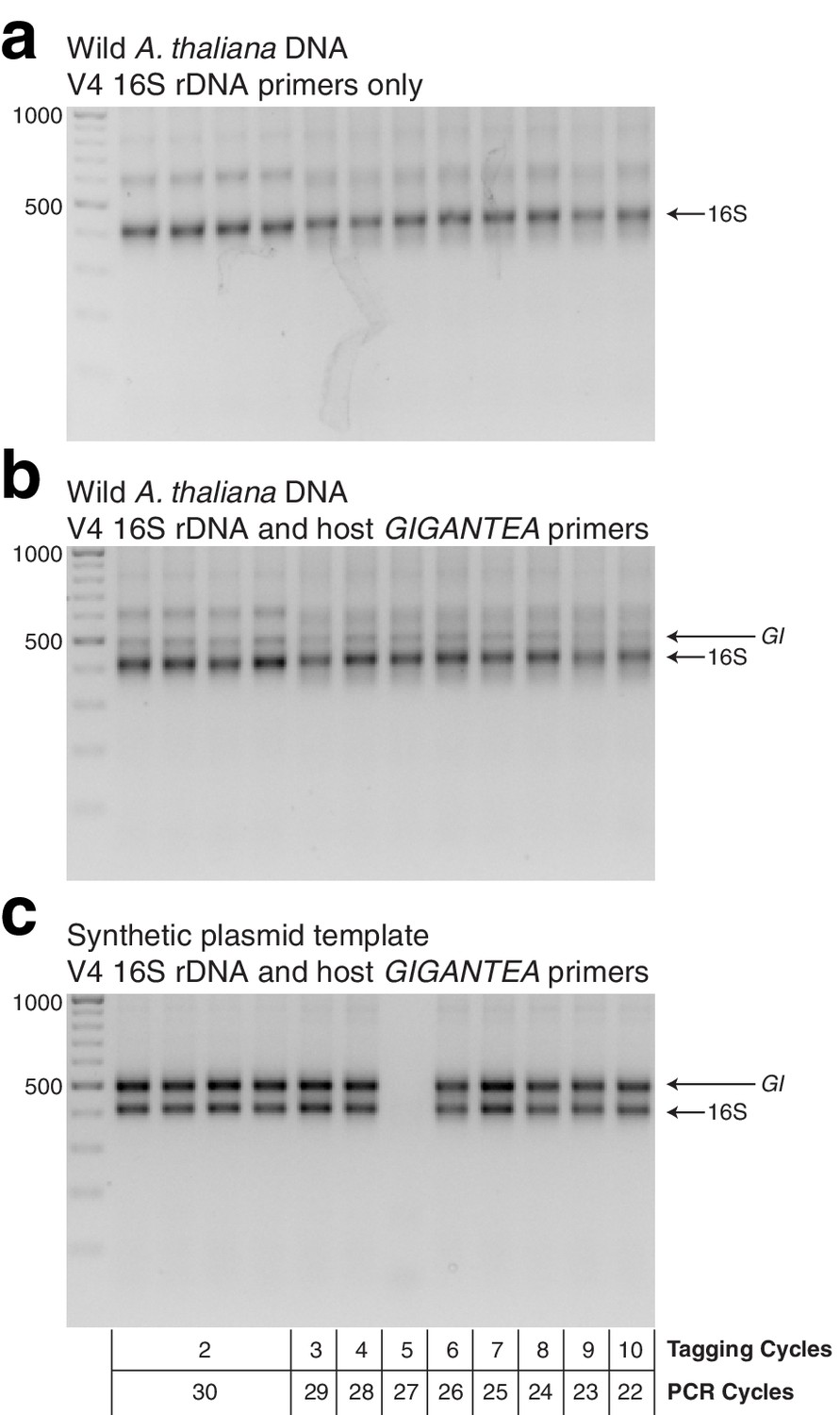
Gel of template HM-tagging cycling tests.
(a) hamPCR using only primers for the V4 region of the 16S rDNA (primers 515F - 799R) was run on pooled DNA made from wild A. thaliana leaves. This represents the output of common two-step 16S rDNA amplification protocols. Four replicates were produced with two cycles of the HM-tagging reaction and 30 cycles PCR, and additional replicates were produced with 3-10 HM-tagging cycles paired with 29 to 22 PCR cycles (for a total of 32 cycles), as shown under panel C. (b) The same DNA, PCR master mix, and cycling conditions as in (a), except with the addition of primers for the 502 bp A. thaliana GI amplicon. (c) The same as in (b), except with a synthetic plasmid template containing a fragment of the A. thaliana GI gene and 16S rDNA from Pst DC3000 in a 1:1 ratio. HM-tagging cycles and PCR cycles for each lane are shown beneath.
Figure 2—figure supplement 2
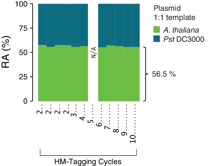
Effect of varying HM-tagging cycles on the plasmid 1:1 host:microbe template.
A synthetic plasmid-borne template including the Pst DC3000 16S rDNA and a portion of the A. thaliana GI gene was used as template for hamPCR using the V4 region of the 16S rDNA (primers 515F - 799R) and the 502 bp A. thaliana GI amplicon. Four replicates were produced with two cycles of the HM-tagging reaction and 30 cycles PCR, and additional replicates were produced with 3-10 HM-tagging cycles paired with 29 to 22 PCR cycles (for a total of 32 cycles). A technical error resulted in no data for 5 HM-tagging cycles (see Figure 2—figure supplement 1). The number of HM-tagging cycles did not influence the ratio of host to microbe, and the host amplicon was slightly, but consistently overrepresented at 56.5% of the total sequence in these samples.
Figure 3 with 2 supplements
After remixing hamPCR amplicons for efficient sequencing, original abundances can be reconstructed.
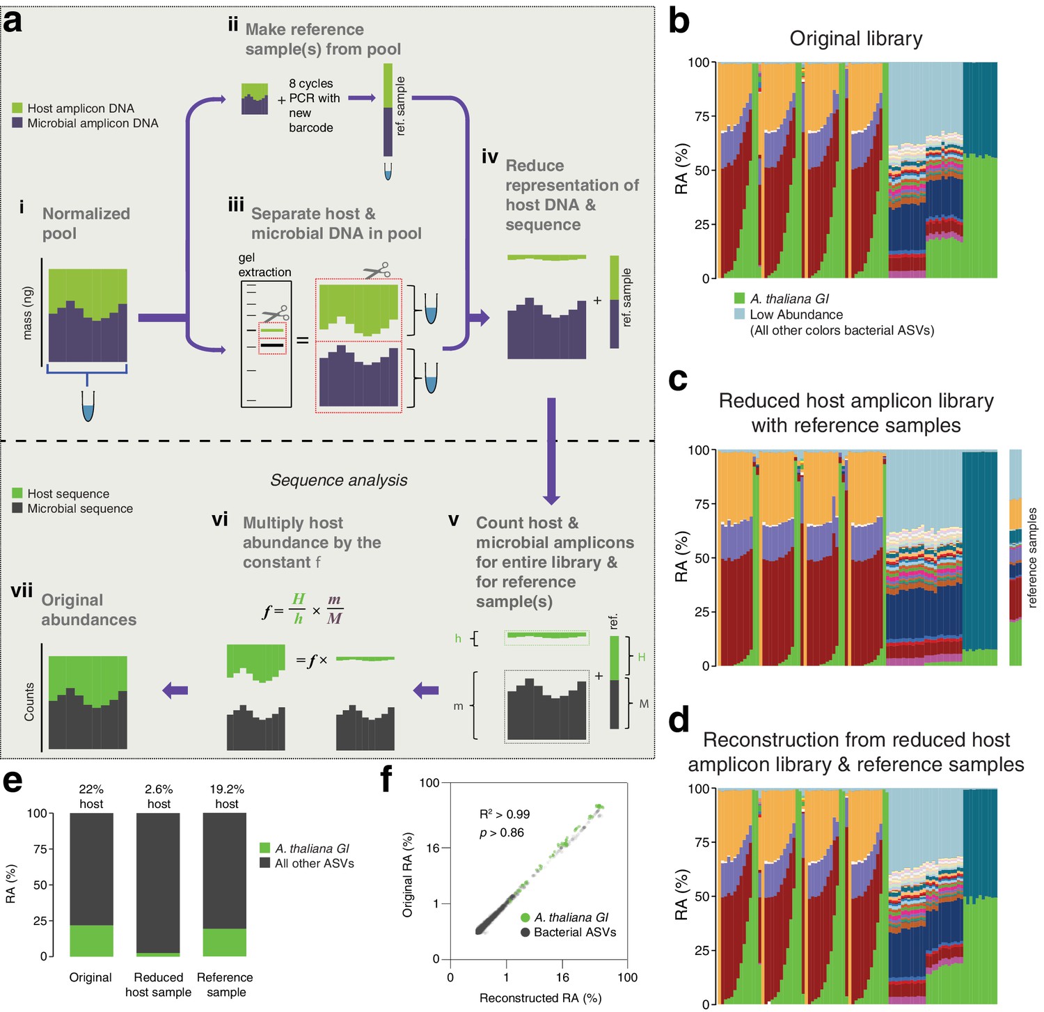
(a) Scheme of remixing process. (i): Products of individual PCRs are pooled at equimolar ratios into a single tube. (ii): An aliquot of DNA from the pool in (i) is re-amplified with eight cycles of PCR to replace all barcodes in the pool with a new barcode, creating a reference sample. (iii): An aliquot of the pool from (i) is physically separated into host and microbial fractions via agarose gel electrophoresis. (iv): The host and microbial fractions and the reference sample are pooled in the ratio desired for sequencing. (v): All sequences are quality filtered, demultiplexed, and taxonomically classified using the same parameters. (vi): Host and microbial amplicon counts are summed from the samples comprising the pooled library (h and m, respectively), and from the reference sample (H and M). (vi): H, h, M, and m are used to calculate the scaling constant f for the dataset. All host sequence counts are multiplied by f to reconstruct the original microbe-to-host ratios. (vii): Reconstructed original abundances. (b) Relative abundance (RA) of actual sequence counts from our original HiSeq 3000 run. (c) Relative abundance of actual sequence counts from our adjusted library showing reduced host and four reference samples. (d) The data from (c) after reconstructing original host abundance using the reference samples. (e) The total fraction of host vs. other ASVs in the original library, reduced host library, and reconstruction. (f) Relative abundances in the original and reconstructed library for all ASVs with a 0.05% minimum abundance, shown on fourth-root transformed axes. R2, coefficient of determination. p-Value from Kolmogorov–Smirnov test.
Figure 3—figure supplement 1

Library remixing prior to sequencing.
(a) PCR products analyzed on a 2% agarose gel. Because the host and microbe amplicons have different lengths, they migrate at different speeds and can be independently resolved. (b) The total DNA concentration of each PCR product is measured. (c) The samples are pooled at equimolar ratios into a single tube. (d) A very small aliquot of the pool from (c) is re-amplified with eight cycles of PCR to replace all barcodes in the pool with a new barcode, creating a reference sample which is set aside. (e) A large aliquot of the pool from (c) is run on an agarose gel to physically separate the host and microbial fractions. These fractions are separately purified and quantified. Because the extraction is done on the pool, samples are not differentially affected by extraction inefficiencies. (f) The DNA concentrations in the host fraction, microbial fraction, and reference sample are each quantified, and the desired molarity of each is aliquoted. Here, host amplicons are depleted to approximately 5% of the total library. The actual mixing ratio is not important, because the reference sample preserves the correct ratio of host to microbe. (g) The reduced host fraction, microbial fraction, and the reference sample are pooled for sequencing. (h) All sequences are quality filtered, demultiplexed, and taxonomically classified using the same parameters. (i) Host and microbe sequence counts are summed from the samples comprising the pooled library (h and m respectively), and from the reference sample (H and M respectively). (j) H, h, M, and m are used to calculate the scaling constant f for the dataset. All host sequence counts are multiplied by f to reconstruct the original microbe-to-host ratios. (k) Reconstructed original abundances (compare to original abundances in B). (l) Finally, each sample is divided by host abundance to normalize host counts, resulting in microbial sequence counts that represent the microbial load of each micobe on the host.
Figure 3—figure supplement 2
Gels and Bioanalyzer traces showing steps of remixing.
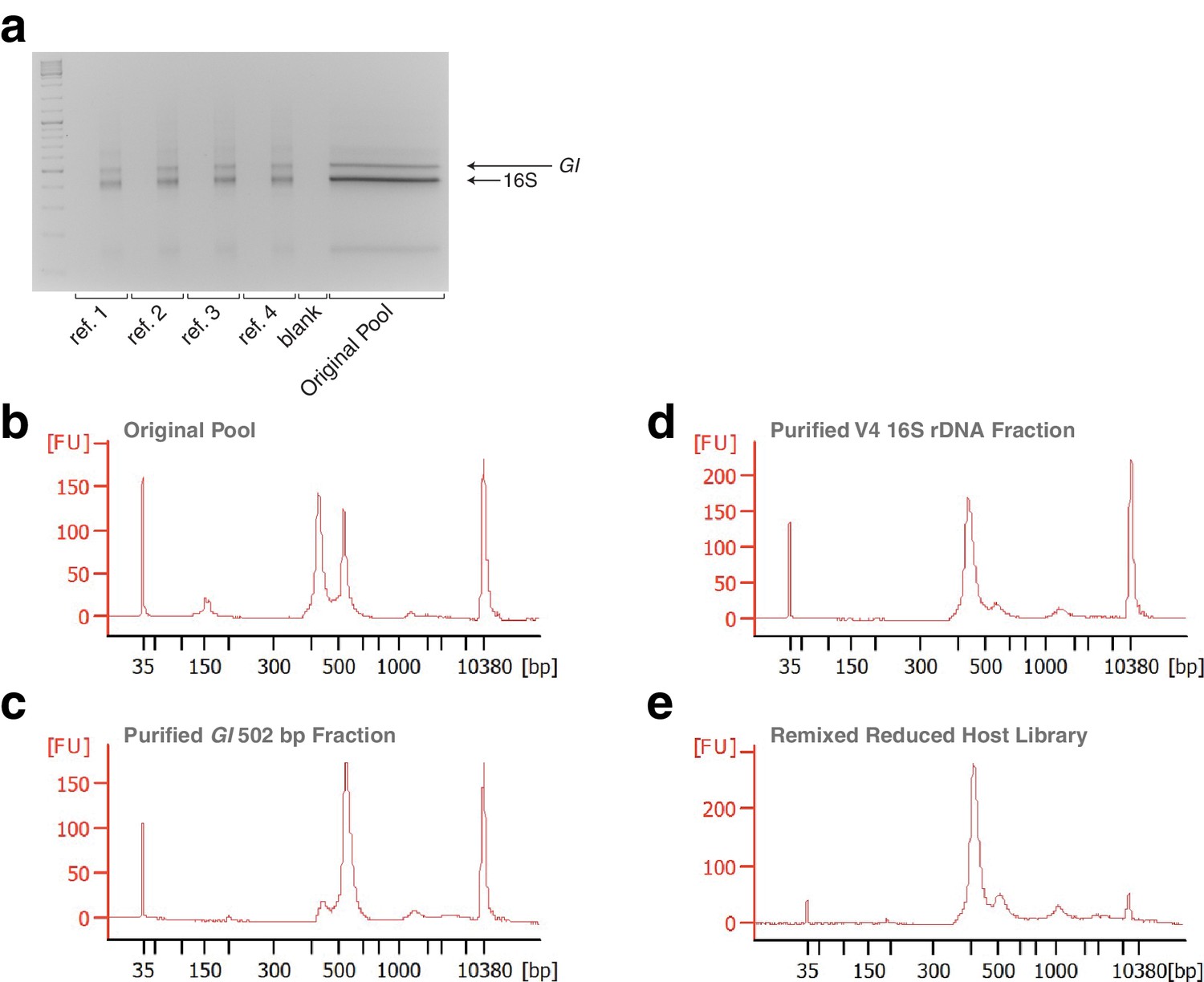
(a) Gel showing four replicate reference samples made from the original pool, confirming successful re-barcoding. For each pair of lanes, the left lane is 5 μL of the PCR reaction prior to eight cycles of amplification, and the right lane is 5 μL after cycling. Size separation of the original pool for purification of the host (GI) and microbial (16S) fractions is shown in the wide lane. (b) Bioanalyzer trace of the original pool, showing nearly equally abundant host and microbial fractions. (c) Bioanalyzer trace of the purified host fraction. While some host fraction has been inadvertently co-purified, this does not influence the overall outcome. (d) Bioanalyzer trace of the purified host fraction. While a small amount of the microbial fraction has been inadvertently co-purified, this does not influence the overall outcome. (e) Bioanalyzer trace of the remixed reduced host library.
Figure 4 with 1 supplement
hamPCR with three common 16S rDNA amplicons gives consistent results that agree with whole metagenome sequencing (WMS).
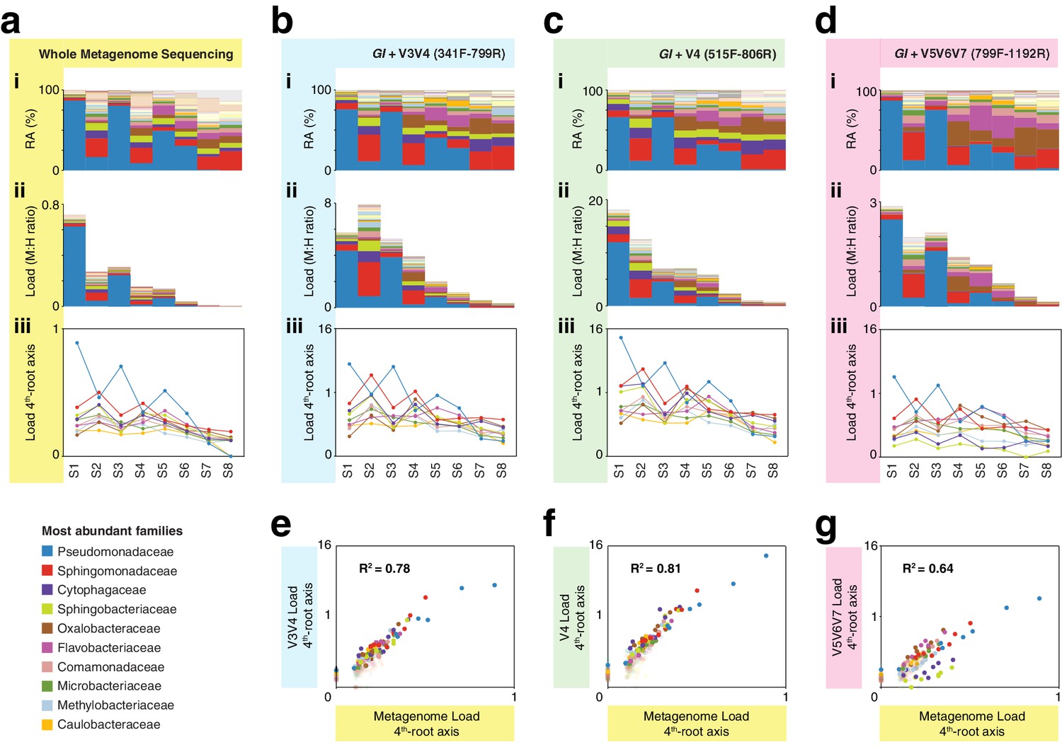
(a) (i): Stacked-column plot showing the relative abundance (RA) of bacterial families in eight wild A. thaliana leaf samples, as determined by WMS. The families corresponding to the first 10 colors from bottom to top are shown in reverse order on the bottom left. (ii) Stacked-column plot showing the bacterial load of the same bacterial families (M:H ratio = microbe-to-host ratio). (iii) The M:H bacterial load ratios for the 10 major bacterial families shown on a fourth-root transformed y-axis. Lines across the independent samples are provided as a help to visualize patterns. (b) Similar to (a), but with abundances resulting from hamPCR targeting a 502 bp A. thaliana GI amplicon and a ~590 bp V3V4 16S rDNA amplicon. (c) Similar to (b), but with the 16S rDNA primers targeting a ~420 bp V4 16S rDNA amplicon. (d) Similar to (b), but with a 466 bp A. thaliana GI amplicon and a ~540 bp V5V6V7 16S rDNA amplicon. (e) Fourth-root transformed abundance of each bacterial family determined by hamPCR of V3V4 16S rDNA plotted against the fourth-root transformed bacterial load from WMS. R2 = Coefficient of determination. (f) Same as (e), but for hamPCR of V4 16S rDNA. (g) Same as (e), but for V5V6V7 16S rDNA.
Figure 4—figure supplement 1

Gel pictures from hamPCR applied to wild A. thaliana leaf DNA samples.
(a) The bacterial load from eight wild A. thaliana samples (Regalado et al., 2020), as determined by shotgun sequencing. (b) Three replicates of hamPCR products made from the same eight DNA samples, using the 502 bp A. thaliana GI amplicon and the ~420 bp V4 16S rDNA amplicon (515F - 806R). The 806R primer was used here instead of the 799R primer used elsewhere in the manuscript so that the 16S rDNA data could be directly compared to previous V4 16S rDNA amplicon data from those samples, which also used 515F - 806R. The products were visualized on a 2% agarose gel. (c) Same as (b), but hamPCR was performed using the ~590 bp V3V4 16S rDNA amplicon (341F - 799R). (d) Same as in (b) and (c), but hamPCR was performed using the 466 bp A. thaliana GI amplicon and the ~540 bp V5V6V7 16S rDNA amplicon (799F - 1192R). Note that in (c) and (d), the bacterial amplicon is longer than the host amplicon.
Figure 5 with 4 supplements
hamPCR can be generalized to more than two amplicons, non-plant hosts, and large or polyploid host genomes.
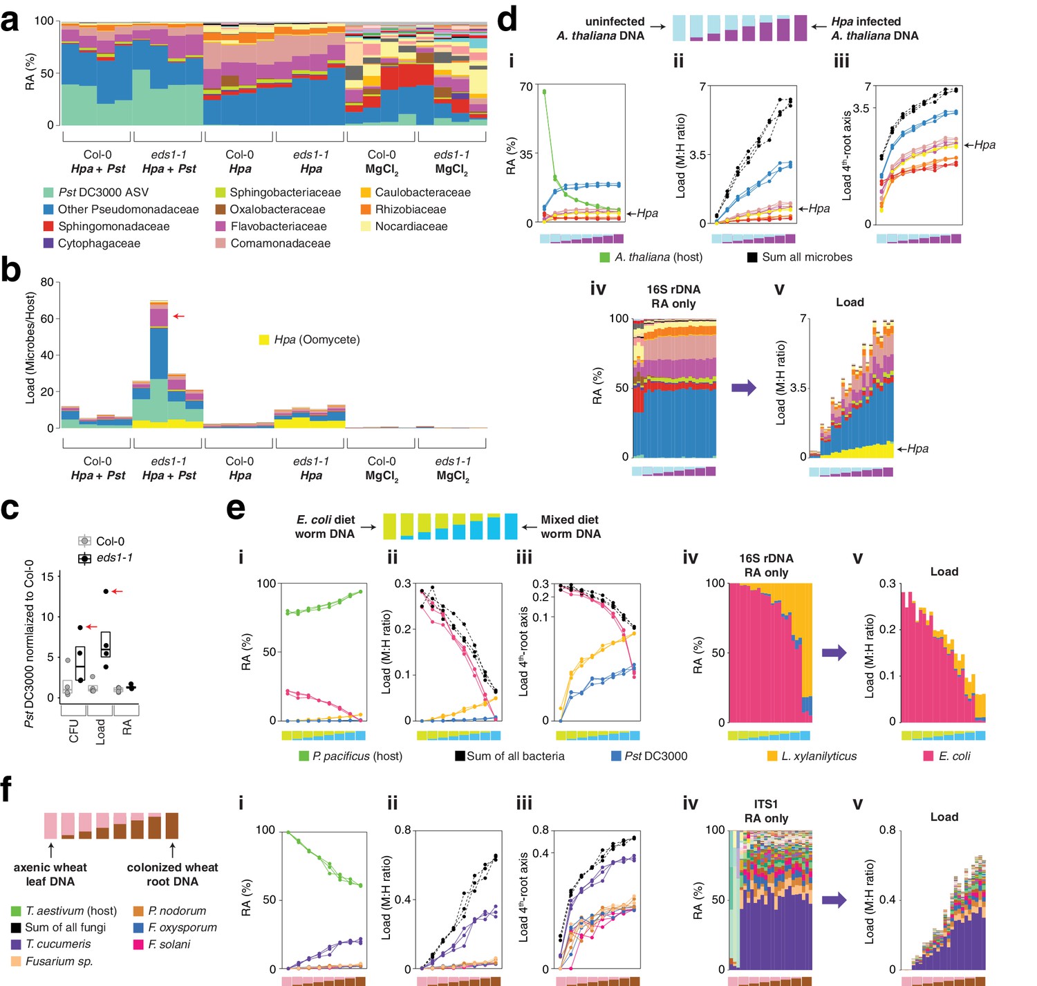
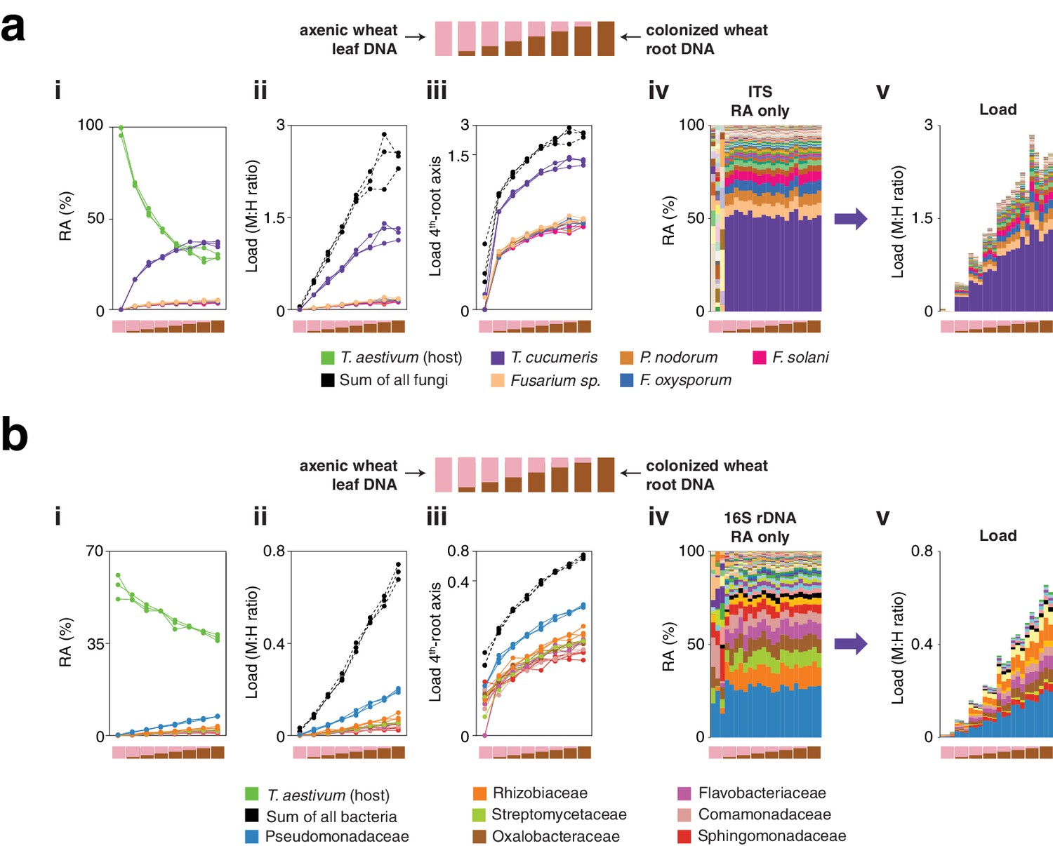
(a) Relative abundance (RA) of only 16S rDNA amplicons for plants co-infected with Hpa and Pst DC3000 and their controls. Each column represents an independent plant. The ASV corresponding to Pst DC3000 (light green) is shown at the bottom and separately from other Pseudomonadaceae; all other bacteria are classified to the family level, including remaining Pseudomonadaceae. Hpa is not detectable using 16S rDNA primers and is therefore not shown. (b) The same data as shown in (a), but making full use of hamPCR by including the ASV for Hpa and converting the combined measurements to microbial load. The red arrow indicates an outlier sample. Same color key as in (a), with an additional color (yellow) for Hpa added. Hpa amplicon abundance was scaled by a factor of 4 in this panel for better visualization. (c) Pst DC3000 bacteria were quantified in parallel on the Col-0 and eds1-1 samples infected with Pst DC3000 using CFU counts, the microbial load data in (b), or the relative abundance data in (a). The median is shown as a horizontal line and box boundaries show the lower and upper quartiles. Red arrows indicate the same outlier sample shown in (b). (d) An uninfected plant sample was titrated into an Hpa-infected sample to make a panel of eight samples. (i): the relative abundance of hamPCR amplicons with median abundance above 0.15%. (ii): after using host ASV to convert amplicons to load. The cumulative load is shown in black. (iii): the load on a fourth-root transformed y-axis, showing less-abundant families. (iv): stacked column visualization of all ASVs for the panel as it would be seen with pure 16S rDNA data. (v): stacked-column plot of the panel corrected for microbial load. Same color key as in (b), but with colors for A. thaliana and sum of microbes added. (e) Similar to (d), but with the nematode worm P. pacificus as host, and V5V6V7 16S rDNA primers. Instead of bacterial families, specific ASV abundances are shown. (f) Similar to (e), but with hexaploid wheat T. aestivum as host, and fungal ASV abundances from ITS1 amplicons.
Figure 5—figure supplement 1

Gel pictures of hamPCR applied to one host and two microbial amplicons.
(a) Test of primer compatibility for primer pairs targeting plant and bacteria, plant and oomycete, or plant and bacteria and oomycete, for the ITSo rDNA amplicon, three alternate bacterial amplicons, and two plant amplicons as shown. Some combinations perform better than others and produce fewer dimers. Shown on a 2% agarose gel. (b) The samples of the Hpa and Pst DC3000 co-infection using ITSo rDNA primers, V4 16S rDNA primers, and 502 bp A. thaliana GI primers. The signal from the ITSo primers overwhelmed the reaction. (c) hamPCR library of the Hpa and Pst DC3000 co-infection as described in Figure 5a-c using Hpa actin primers, V4 16S rDNA primers, and 502 bp A. thaliana GI primers. (d) hamPCR libraries made with the titration of plant DNA infected with Hpa as described in Figure 5d, using actin primers, V4 16S rDNA primers, and 502 bp A. thaliana GI primers.
Figure 5—figure supplement 2

Gel of P. pacificus hamPCR titration libraries.
DNA was prepared from two populations of P. pacificus strain PS312, one fed with only E. coli and another fed with E. coli, P. syringae, and Lysinibacillus xylanilyticus (mixed diet). The two DNA samples were each adjusted to 6 ng/μL and titrated into each other using the ratios shown below the gel. The 2% agarose gel shows resulting hamPCR libraries using the ~540 bp V5V6V7 16S rDNA amplicon (primers 799F - 1192R) and the 470 bp P. pacificus calsequestrin (csq-1) amplicon.
Figure 5—figure supplement 3
Gels of T. aestivum hamPCR titration libraries.
(a-c) DNA was made from axenic T. aestivum leaf DNA and surface-sterilized T. aestivum roots that had been cultivated outdoors in potting soil. The two DNA samples were each adjusted to ~60 ng/μL and titrated into each other using the ratios shown below the gel. hamPCR products are displayed on a 2% agarose gel. (a) hamPCR products using the ITS1 fungi amplicon and the 497 bp T. aestivum PolA1 amplicon. The ITS1 and PolA1 primer pairs were mixed in a 1:1 ratio. HM-tagging was performed with two cycles and PCR was performed with 30 cycles. Note that ITS1 amplicons form a smear on the gel due to a wide range of amplicon sizes. (b) Same as (a), but the ITS1 and PolA1 primer pairs were mixed in a 2:1 ratio to favor ITS1 amplification. To help amplification of lower quantities of tagged templates, HM-tagging was performed with seven cycles and PCR was performed with 25 cycles. (c) hamPCR products using primers for V4 16S rDNA from bacteria (primers 515F - 799R) and the 497 bp T. aestivum PolA1 amplicon. A standard protocol of 2 HM-tagging cycles and 30 PCR cycles was used.
Figure 5—figure supplement 4

ITS1 load in T. aestivum with a 2:1 microbe-to-host HM-tagging primer ratio, and 16S rDNA load in T. aestivum.
(a) Similar to Figure 5f in the main text, axenic T. aestivum leaf DNA was titrated into DNA from T. aestivum roots that had been cultivated outdoors in potting soil to make a panel of eight samples simulating different levels of infection. hamPCR was performed for three replicates per sample using ITS1 fungal primers and T. aestivum PolA1 primers. Unlike Figure 5f, the ITS1 and PolA1 primer pairs were mixed in a 2:1 ratio to favor ITS1 amplification, and HM-tagging was performed with seven cycles and PCR was performed with 25 cycles. (i) The relative abundance of hamPCR amplicons with median abundance above 0.15%. (ii) After using host ASV to convert amplicons to load. The cumulative load is shown in black. (iii) The load on a fourth-root transformed y-axis, showing less abundant families. (iv) Stacked column visualization of all ASVs for the panel as it would be seen with pure ITS1 data. v: stacked-column plot of the panel corrected for microbial load. (b) Loads for abundant fungal ASVs following hamPCR with a 2:1 ITS1 to PolA1 primer ratio plotted against loads for the same ASVs following hamPCR with a 1:1 ITS1 to PolA1 primer ratio (as displayed in Figure 5f). Shown on fourth-root axes. R2, coefficient of determination. The correlation comparing ASVs in 1:1 and 2:1 ITS1 to PolA1 primer ratios is just as high as for the correlation between technical replicates with the same priming conditions, shown next in (c) and (d). (c) Same as (b), but with one technical replicate of hamPCR with a 1:1 ITS1 to PolA1 primer ratio plotted against a second technical replicate of the 1:1 ratio. (d) Same as (b) and (c), but for one technical rep of hamPCR with a 2:1 ITS1 to PolA1 primer ratio plotted against a second technical replicate of the 2:1 ratio. (e) hamPCR using the V4 16S rDNA bacterial amplicon and the T. aestivum PolA1 amplicon, using a standard 1:1 microbe-to-host primer ratio and normal cycling. Subpanels i-v as in (a), with bacterial families shown instead of fungal ASVs.
Figure 6 with 2 supplements
hamPCR can provide new insights into microbial interactions in crop plants.
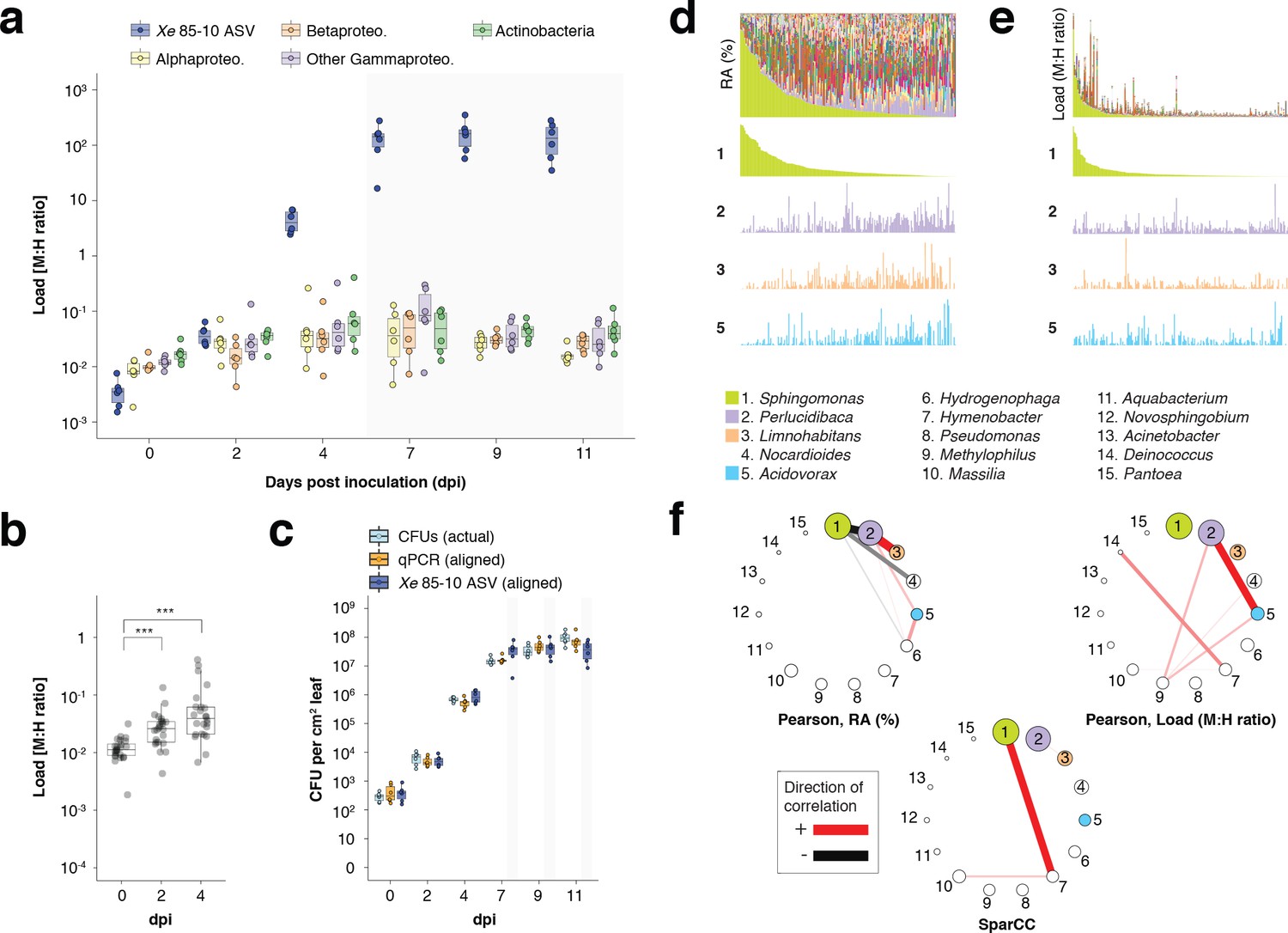
(a–c) C. annuum growth curve experiment. All y-axes are on a base-10 logarithmic scale. In all boxplots, the median is represented by a horizontal line and box boundaries show the lower and upper quartiles. Whiskers extend from the box up to 1.5 times the interquartile range. (a) Xe 85–10 was inoculated into C. annuum leaves at 104 CFU/mL. Leaf samples were taken at 0, 2, 4, 7, 9, and 11 days post inoculation (dpi), and hamPCR performed. The corrected load is shown for the particular ASV corresponding to Xe 85–10, as well as for the major bacterial classes. (b) The total load for all bacterial classes shown in a at 0, 2, and 4 dpi (***p<0.001, Mann-Whitney U-test). (c) Actual CFU counts for Xe 85–10 in the growth curve experiment juxtaposed with scaled qPCR and hamPCR loads. (d-e) Field-grown Z. mays collection. (d) Relative abundance (RA) of bacterial genera found in Z. mays leaf hole punches, ordered by Sphingomonas relative abundance. The genera corresponding to the first 15 colors from bottom to top are shown in reverse order in the legend. The relative abundance of four isolated genera is highlighted (colored boxes in legend). (e) Same as (d) but showing microbial load rather than relative abundance and ordered by Sphingomonas load. (f) Correlation networks of the same 15 genera from the legend for d and e. Pearson correlation from RA data from d (left), pearson correlation of microbial load from e (right), and SparCC correlation network (bottom). Circles representing genera are scaled such that their area represents the median genus abundance across all samples. Only correlations of absolute magnitude >= 0.3 are shown.
Figure 6—figure supplement 1

Gels from C. annuum experiments.
(a) Two percent agarose gel showing hamPCR libraries for four replicates of C. annuum infiltration with Xanthomonas euvesicatoria (Xe) 85-10. The HM-tagging step was done with V4 16S rDNA primers (515F - 799R) and C. annuum GI primers. (b) Two percent agarose gel showing hamPCR libraries for six replicates per timepoint of a C. annuum growth curve following infiltration with 104 228 CFU/mL Xe 85-10.
Figure 6—figure supplement 2
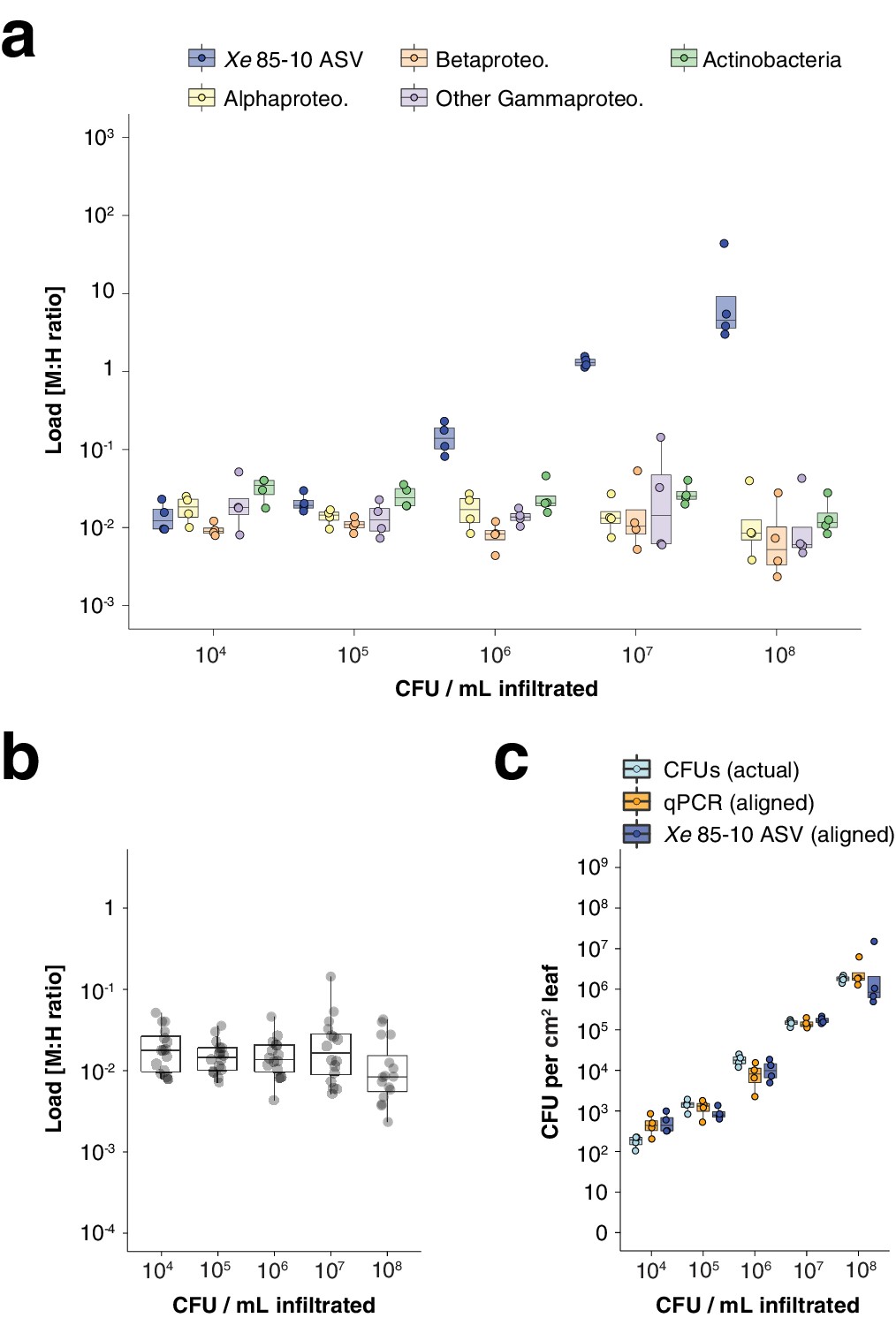
hamPCR can be generalized to Xanthomonas infection of C. annuum.
(a-c) Infiltration experiment. All y-axes are on a base-10 logarithmic scale. In all boxplots, the median is represented by a horizontal line and box boundaries show the lower and upper quartiles. Whiskers extend from the box up to 1.5 times the interquartile range. (a) Xe 85-10 was inoculated into C. annuum leaves at five concentrations, leaves were harvested immediately afterwards, and hamPCR was performed. The bacterial load is shown for the particular ASV corresponding to Xe 85-10, as well as for the major bacterial classes. (b) The total load for all bacterial classes shown in (a) at each concentration. (c) Actual CFU counts for Xe 85-10 in the infiltration experiment juxtaposed with aligned qPCR and hamPCR loads.
Appendix 1—figure 1
PCR Scheme.
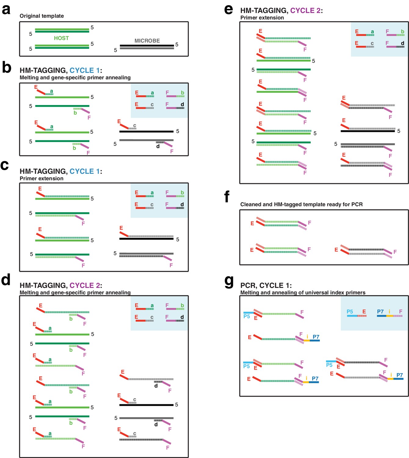
(a) The input DNA is shown as two double-stranded DNA molecules from the host (light/dark green) and one double-stranded DNA molecule from a microbe (black/gray). (b) In the annealing step of HM-tagging cycle one, an excess of two primer pairs is present (blue box), each with a gene-specific region (regions a through d) and universal overhangs (regions E and F). The gene-specific regions of each primer anneal to the templates. (c) In the extension step of HM-tagging cycle 1, primers are extended to make a single copy of each template molecule with a universal overhang on the 5’ end, producing ‘single-tagged templates’. Extended molecules are represented by dashed lines, while original templates retain a solid line. (d) In HM-tagging cycle 2, again the gene-specific regions of each primer anneal to all template molecules, both to the originals and single-tagged templates. (e) In the extension step, note that for those primers that had annealed to single-tagged templates, extension generates the reverse complement of the universal overhang, producing ‘double-tagged templates’. (f) Primers are removed from the reaction with SPRI beads prior to PCR. Note that the quantity of double-tagged template molecules is the same as the quantity of original template molecules. Although original template and single-tagged templates survive SPRI cleanup and are also present in this step, these lack the universal overhangs and cannot be amplified in PCR and are not shown. (g) For the exponential PCR step, an excess of a single primer pair is present (blue box), each with a region complementary to the universal overhangs (regions E and F) and sequencing adapters (regions P5 and P7). An index for multiplexing is present on one or both primers (region i). Because double-tagged templates from both host and microbe have the same universal overhangs, they are not differentially amplified during PCR.
Appendix 1—figure 2

SPRI ratios.
SPRI beads in a polyethylene glycol (PEG) solution, such as AMPure XP, preferentially bind longer DNA fragments, making them useful for removing free primers and primer dimers from reactions. As the PEG concentration decreases, a wider range of short fragments can no longer bind to the beads, and primer dimers are more completely eliminated. However, if the PEG concentration is too low, the range of fragment sizes eliminated could include DNA of interest. For hamPCR, it is important that the SPRI cleanup does not affect the ratio of the host and microbial amplicons, which could lead to systematic bias and noise. To determine an acceptable PEG concentration, we tested cleanups with SPRI (AMPure XP) beads at different SPRI: DNA ratios (resulting in a range of PEG concentrations) on a standard DNA size ladder (GeneRuler DNA Ladder Mix, Thermo Scientific, Waltham, MA, USA), and quantified abundance of the purified fragments with a Bioanalyzer (Agilent, Santa Clara, CA, USA). Using the pure, uncleaned ladder, we calculated the ratio of each peak’s abundance to the adjacent larger peak (200: 300 bp, 300: 400 bp, etc.), and used this set of abundance ratios as a baseline (no SPRI, far left). With each successive decrease in SPRI: DNA ratio (from left to right), we looked for a decrease in the abundance ratio between adjacent bands, which would indicate elimination of the smaller fragment. Of highest interest is the 300: 400 bp ratio (black), because the smallest tagged templates in hamPCR are around 300 bp. We determined SPRI: DNA ratios less than 1.0 endangered the 300: 400 ratio, and thus decided to conservatively use a SPRI: DNA solution of 1.1: 1 or higher for the cleanup of tagged products.
Appendix 1—figure 3
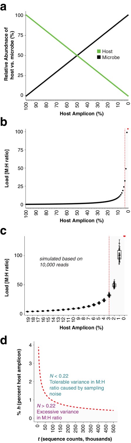
In silico load simulations.
(a), One hundred and one samples were simulated by combining 0 to 100 microbial sequence counts (black points) with 100 to 0 sequence counts (green points). The x-axis shows the percentage of the sample occupied by the host amplicon, decreasing from left to right. The lines show a simple linear, mutually-exclusive relationship between host and microbe. (b) The microbial abundances from (a) were converted to microbial load by dividing by the host abundances. Note that as the host amplicon abundance approaches 0, the microbial load climbs towards infinity. The red point at 0% host amplicon abundance represents infinite load. The vertical red dotted line indicates 3% host amplicon abundance; below 3% host abundance, load becomes extremely sensitive to small changes in host abundance. (c) The 100 plant and microbial sequence counts for each sample in (a) were multiplied by 10,000 to make virtual samples with 1 million sequence counts. These were then subsampled 50 times each to 10,000 reads to simulate samples with random sampling noise. Microbial load from the virtual samples was calculated as in (b) by dividing microbial counts by host counts. Only host amplicon percentages from 19% to 0% are shown to focus on lower host abundances. The red point at 0% host amplicon abundance represents infinite load. The vertical red dotted line indicates the position of 3% host amplicon abundance. Note that not only does load climb quickly towards infinity as host counts approach 0, but also sampling noise has a greater impact on microbial load. (d) Deeper sequencing reduces the variance in microbial load associated with a low abundance host amplicon by reducing the impact of sampling noise. We defined a noise level, N, as the range in calculated microbial load that would result from subtracting one sequence count from the host and assigning it to a microbe, and vice versa, as shown in the following equation, where M and H are integer sequence counts of microbe and host, respectively: . For 10,000 reads with a host percentage of 3% (300 counts) as shown by the red line in (c), we calculate N = 0.22 and suggest it as an upper limit. To visualize how deeper sequencing enables lower host amplicon abundances without increasing noise, we plotted the relative abundance of the host amplicon as a function of sequencing depth (red dotted line), maintaining N = 0.22 as shown in the following equation, where t is the total reads in each sample and % h is the percent of host amplicon. . Combinations of host amplicon abundances and sequencing depths below this line (gray area) are less reliable, and not recommended for quantitative conclusions.
Appendix 1—figure 4
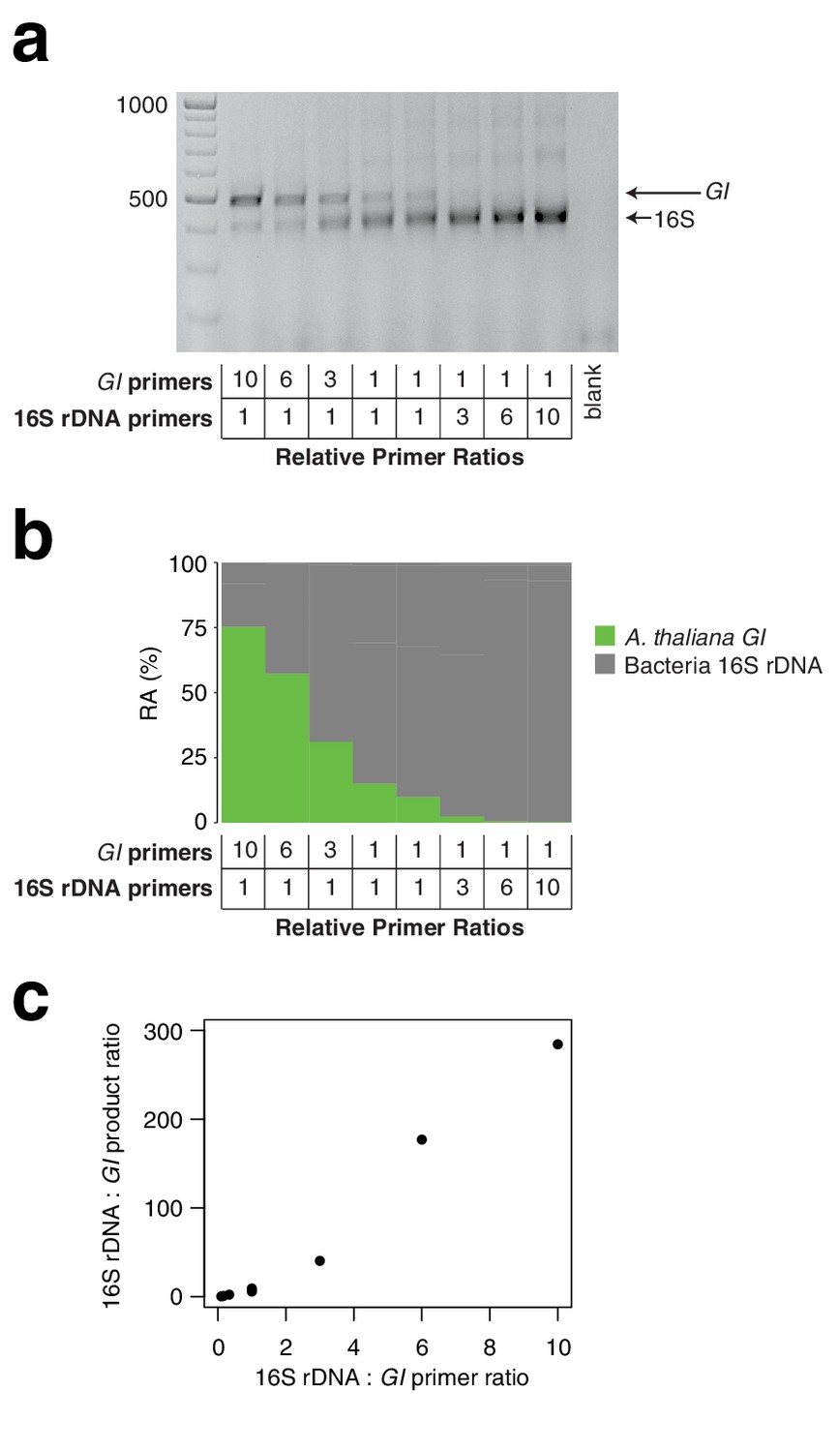
Effect of primer pair concentration on product.
The same wild A. thaliana DNA pool was amplified with hamPCR using eight different ratios of the 16S rDNA primer pair to the GI primer pair, ranging from 1/10 to 10. (a) 2% agarose gel of the prepared libraries (b) Relative abundance (RA) of bacteria and host amplicons in the sequence data. (c) Scatterplot of microbe-to-host product ratios plotted against the microbe-to-host primer ratios used to produce them. A tenfold difference in primer ratios resulted in an over 200-fold difference in product ratios, underscoring the importance of steady primer ratios (through the use of a mastermix of primers) across an experiment.
Appendix 1—figure 5
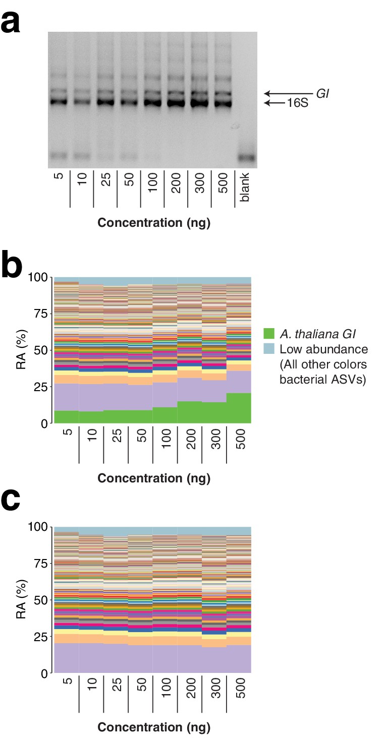
Total template concentration test.
A panel of eight concentrations of wild A. thaliana leaf DNA, ranging from 5 to 500 ng per reaction (approximately 3.6×10⁴ to 3.6×10⁶ host GI template copies per reaction assuming a 135 Mb A. thaliana genome), were converted into hamPCR libraries. (a) 2% agarose gel of the prepared libraries. (b) Relative abundance (RA) of all amplicons in the reaction. The A. thaliana GI ASV appears to increase at the highest template concentrations, but remains of constant abundance through the standard template range of 5–100 ng. (c) The A. thaliana GI ASV has been removed and the bacterial ASVs have been rescaled to give bacterial relative abundance.
Appendix 1—figure 6
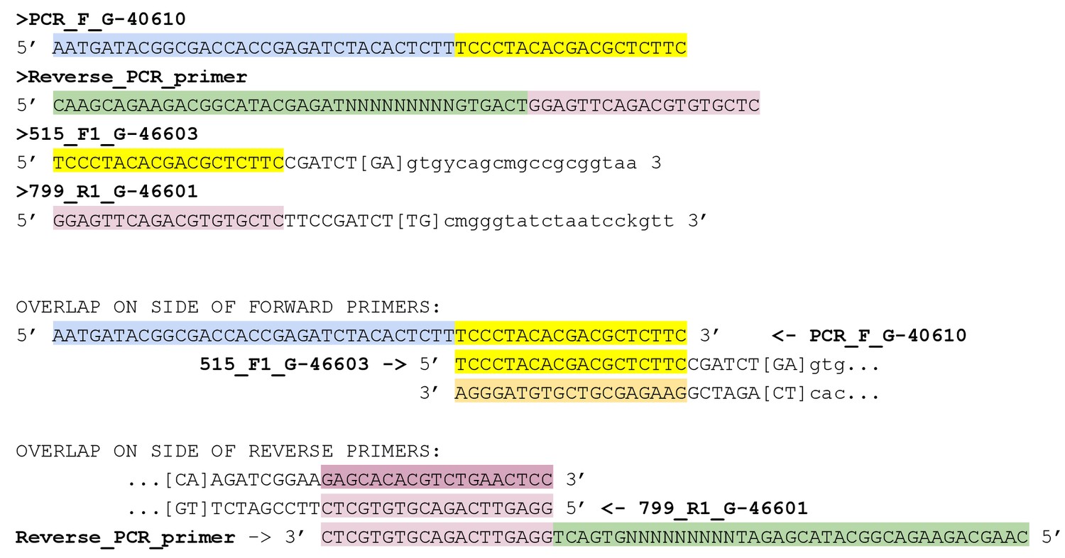
Alignment of PCR primers with HM-tagged templates.
Tables
Key resources table
| Reagent type (species) or resource | Designation | Source or reference | Identifiers | Additional information |
|---|---|---|---|---|
| Sequence-based reagent | HM-tagging primers | Eurofins; this paper | Standard desalting; for sequences see Supplementary file 1, Appendix 1 | |
| Sequence-based reagent | PCR forward primer | Eurofins; https://doi.org/10.1017/qpb.2020.6 | PCR_F_G-40610 | 5’-AATGATACGGCGACCACCGA GATCTACACTCTTTCCCTACA CGACGCTCTTC-3’; HPLC purified |
| Sequence-based reagent | PCR reverse primers | IDT; https://doi.org/10.1038/nmeth.2634 | IDT Ultramers; for sequences see Supplementary file 1 | |
| Sequence-based reagent | XopQ Xanthomonas qPCR primers | Eurofins; https://doi.org/10.1038/s41598-019-46588-9; | XopQ_F, XopQR | 5’-GCGAGGAACTTGGAATGCTC-3’ 5’-AGGCCGAAGGCTTTTTGCG-3’; Standard desalting |
| Sequence-based reagent | UBI3 C. annuum qPCR primers | Eurofins; https://doi.org/10.1016/j.bbrc.2011.10.105 | UBI3_F, UBI3_R | 5’-TGTCCATCTGCTCTCTGTTG-3’ 5’-CACCCCAAGCACAATAAGAC-3’; Standard desalting |
| Peptide, recombinant protein | Taq DNA Polymerase | NEB | Cat. #: M0267 | |
| Peptide, recombinant protein | Q5 DNA Polymerase | NEB | Cat. #: M0491 | |
| Peptide, recombinant protein | pPNA, mPNA | PNAbio | Cat. #: PP01, MP01 | Peptide nucleic acids for blocking organelle amplification when using hamPCR on plants. |
| Software, algorithm | USEARCH | www.drive5.com | version 11 | |
| Recombinant DNA reagent | Synthetic equimolar plasmid template (plasmid) | This paper | For sequence and construction, see Appendix 1 - Discussion 2. | |
| Other | Solid phase reversible immobilization (SPRI) beads | https://dx.doi.org/10.1101%2Fgr.128124.111 |
Additional files
-
Supplementary file 1
Primers, metadata, and other raw data.
This file is an excel sheet with six subtables as tabs. These are: 'Tagging Primers', 'PCR Primers', 'qPCR Primers', 'Sample Metadata', 'Pepper qPCR raw data', and 'Pepper CFU raw data'.
- https://cdn.elifesciences.org/articles/66186/elife-66186-supp1-v2.xlsx
-
Transparent reporting form
- https://cdn.elifesciences.org/articles/66186/elife-66186-transrepform-v2.docx
Download links
A two-part list of links to download the article, or parts of the article, in various formats.
Downloads (link to download the article as PDF)
Open citations (links to open the citations from this article in various online reference manager services)
Cite this article (links to download the citations from this article in formats compatible with various reference manager tools)
Host-associated microbe PCR (hamPCR) enables convenient measurement of both microbial load and community composition
eLife 10:e66186.
https://doi.org/10.7554/eLife.66186


