Figures and data in Natural-gradient learning for spiking neurons

Figures
Tables
Additional files

12 figures, 1 table and 2 additional files

Figures

Figure 1

Download asset Open asset

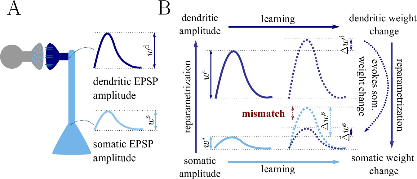
Classical gradient descent depends on chosen parametrization.

(A) The strength of a synapse can be parametrized in various ways, for example, as the EPSP amplitude at either the soma $w^{s}$ or the dendrite $w^{d}$ . Biological processes such as attenuation govern the relationship between these variables. Depending on the chosen parametrization, Euclidean-gradient descent can yield different results. (B) Phenomenological correlates. EPSPs before learning are represented as continuous, after learning as dashed curves. The light blue arrow represents gradient descent on the error as a function of the somatic EPSP $C^{s} [w^{s}]$ (also shown in light blue). The resulting weight change leads to an increase $Δ w^{s}$ in the somatic EPSP after learning. The dark blue arrows track the calculation of the same gradient, but with respect to the dendritic EPSP (also shown in dark blue): (1) taking the attenuation into account in order to compute the error as a function of $w^{d}$ , (2) calculating the gradient, followed by (3) deriving the associated change in $\tilde{Δ} w^{s}$ , again considering attenuation. Due to the attenuation $f (w)$ entering the calculation twice, the synaptic weights updates, as well as the associated evolution of a neuron’s output statistics over time, will differ under the two parametrizations.

Figure 2

Download asset Open asset

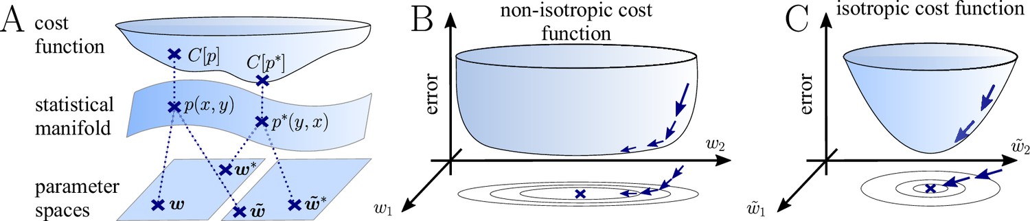
The natural gradient represents the true gradient direction on the manifold of neuronal input-output distributions.

(A) During supervised learning, the error between the current and the target state is measured in terms of a cost function defined on the neuron’s output space; in our case, this is the manifold formed by the neuronal output distributions $p (y, x)$ . As the output of a neuron is determined by the strength of incoming synapses, the cost $C$ depends indirectly on the afferent weight vector $w$ . Since the gradient of a function depends on the distance measure of the underlying space, Euclidean-gradient descent, which follows the gradient of the cost as a function of the synaptic weights $\partial C / \partial w$ , is not uniquely defined, but depends on how $w$ is parametrized. If, instead, we follow the gradient on the output manifold itself, it becomes independent of the underlying parametrization. Expressed in a specific parametrization, the resulting natural gradient contains a correction term that accounts for the distance distortion between the synaptic parameter space and the output manifold. (**B–C**) Standard gradient descent learning is suited for isotropic (C), rather than for non-isotropic (B) cost functions. For example, the magnitude of the gradient decreases in valley regions where the cost function is flat, resulting in slow convergence to the target. A non-optimal choice of parametrization can introduce such artefacts and therefore harm the performance of learning rules based on Euclidean-gradient descent. In contrast, natural-gradient learning will locally correct for distortions arising from non-optimal parametrizations (see also Figure 3).

Figure 3

Download asset Open asset

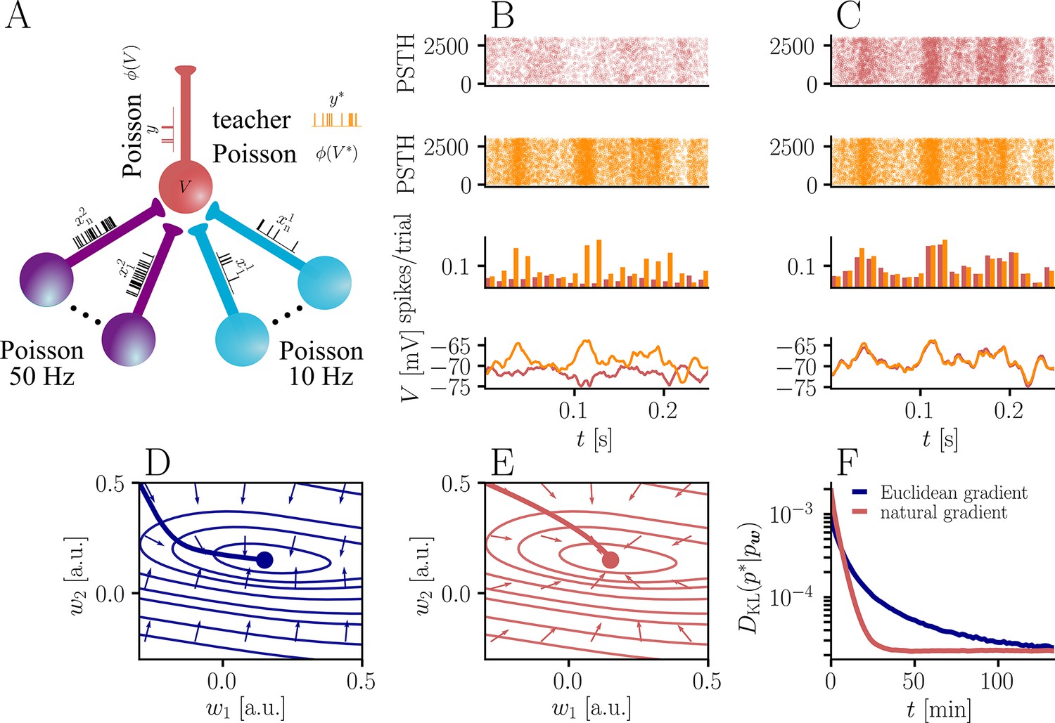
Natural-gradient plasticity speeds up learning in a simple regression task.

(A) We tested the performance of the natural gradient rule in a supervised learning scenario, where a single output neuron had to adapt its firing distribution to a target distribution, delivered in form of spikes from a teacher neuron. The latter was modeled as a Poisson neuron firing with a time-dependent instantaneous rate, $ϕ (\sum_{i = 1}^{n} w_{i}^{*} x_{i}^{ϵ})$ where $w^{*}$ represents a randomly chosen target weight vector. The input consisted of Poisson spikes from $n$ afferents, half of them firing at 10 Hz and 50 Hz, respectively. For our simulations, we used $n = 100$ afferents, except for the weight path plots in (D) and (E), where the number of afferents was reduced to $n = 2$ for illustration purposes. (**B–C**) Spike trains, PSTHs and voltage traces for teacher (orange) and student (red) neuron before (B) and after (C) learning with natural-gradient plasticity. During learning, the firing patterns of the student neuron align to those of the teacher neuron. The structure in these patterns comes from autocorrelations in this instantaneous rate. These, in turn, are due to mechanisms such as the membrane filter (as seen in the voltage traces) and the nonlinear activation function. (**D–E**) Exemplary weight evolution during Euclidean-gradient (D) and natural-gradient (E) learning given $n = 2$ afferents with the same two rates as before. Here, $w_{1}$ corresponds to $x^{1}$ in panel A (10 Hz input) and $w_{2}$ to $x^{2}$ (50 Hz input). Thick solid lines represent contour lines of the cost function $C$ . The respective vector fields depict normalized negative Euclidean and natural gradients of the cost $C$ , averaged over 2000 input samples. The thin solid lines represent the paths traced out by the input weights during learning averaged over 500 trials. (F) Learning curves for $n = 100$ afferents using natural-gradient and Euclidean-gradient plasticity. The plot shows averages over 1000 trials with initial and target weights randomly chosen from a uniform distribution $U (- 1 / n, 1 / n)$ . Fixed learning rates were tuned for each algorithm separately to exhibit the fastest possible convergence to a root mean squared error of 0.8 Hz in the student neuron’s output rate.

Figure 4

Download asset Open asset

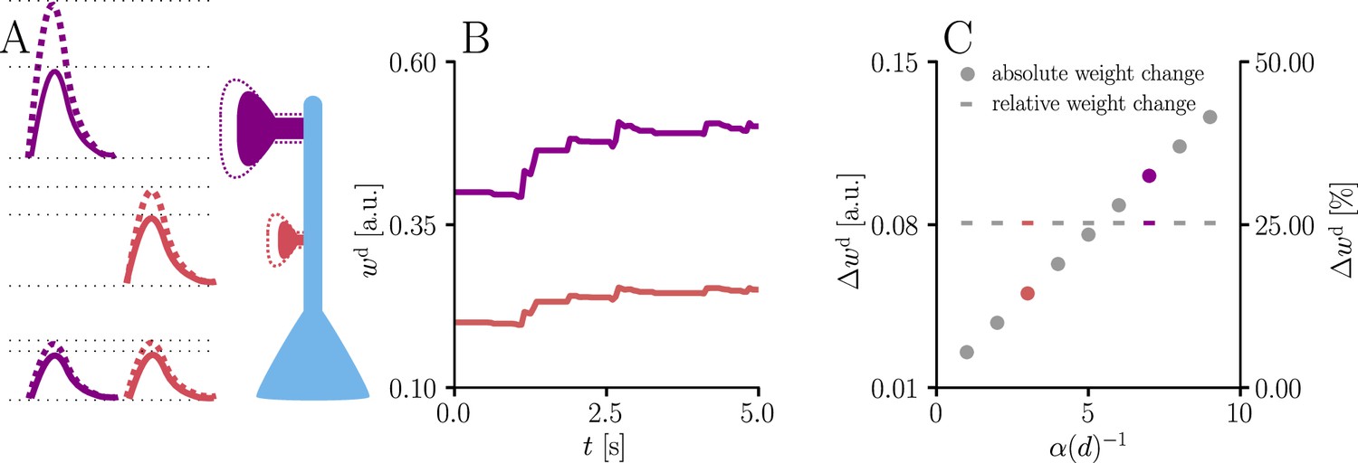
Natural-gradient learning scales synaptic weight updates depending on their distance from the soma.

We stimulated a single excitatory synapse with Poisson input at 5 Hz, paired with a Poisson teacher spike train at 20 Hz. The distance d from soma was varied between 0 μm and 460 μm and attenuation was assumed to be linear and proportional to the inverse distance from soma. To make weight changes comparable, we scaled dendritic PSP amplitudes with $α {(d)}^{- 1}$ in order for all of them to produce the same PSP amplitude at the soma. (A) Example PSPs before (solid lines) and after (dashed lines) learning for two synapses at 3 μm and 7 μm. Application of our natural-gradient rule results in equal changes for the somatic PSPs. (B) Example traces of synaptic weights for the two synapses in (A). (C) Absolute and relative dendritic amplitude change after 5 s as a function of a synapse’s distance from the soma.

Figure 5

Download asset Open asset

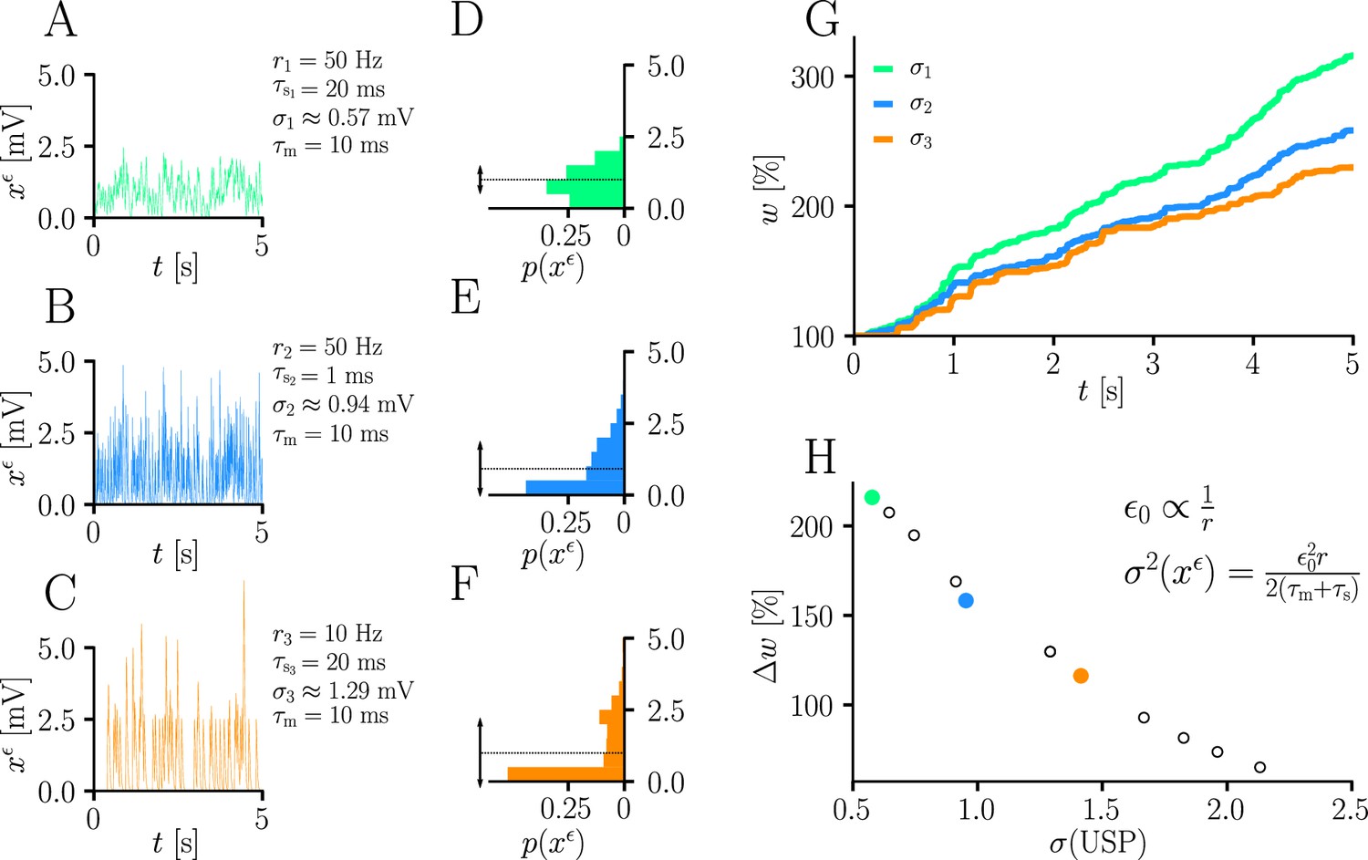
Natural-gradient learning scales approximately inversely with input variance.

(**A–C**) Exemplary USPs $x_{i}^{ϵ}$ and (**D–F**) their distributions for three different scenarios between which the USP variance $σ^{2} (x_{i}^{ϵ})$ is varied. In each scenario, a neuron received a single excitatory input with a given rate $r$ and synaptic time constant $τ_{s}$ . The soma always received teacher spikes at a rate of 80 Hz. To enable a meaningful comparison, the mean USP was conserved by appropriately rescaling the height $ϵ_{0}$ of the USP kernel $ϵ$ (see Sec. ‘Neuron model’). (**A,D**) Reference simulation. (**B,E**) Reduced synaptic time constant, resulting in an increased USP variance $σ_{2}^{2}$ . (**C,F**) Reduced input rate, resulting in an increased USP variance $σ_{3}^{2}$ . (G) Synaptic weight changes over 5 s for the three scenarios above. (H) Total synaptic weight change after $t_{0} = 5 s$ as a function of USP variance. Each data point represents a different pair of $r$ and $τ_{s}$ . The three scenarios above are marked with their respective colors.

Figure 6

Download asset Open asset

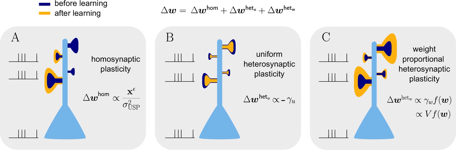
Natural-gradient learning combines multiple forms of plasticity.

Spike trains to the left of the neuron represent afferent inputs to two of the synapses and teacher input to the soma. The two synapses on the right of the dendritic tree receive no stimulus. The teacher is assumed to induce a positive error. (A) The homosynaptic component adapts all stimulated synapses, leaving all unstimulated synapses untouched. (B) The uniform heterosynaptic component changes all synapses in the same manner, only depending on global activity levels. (C) The proportional heterosynaptic component contributes a weight change that is proportional to the current synaptic strength. The magnitude of this weight change is approximately proportional to a product of the current membrane potential above baseline and the weight vector.

Figure 7

Download asset Open asset

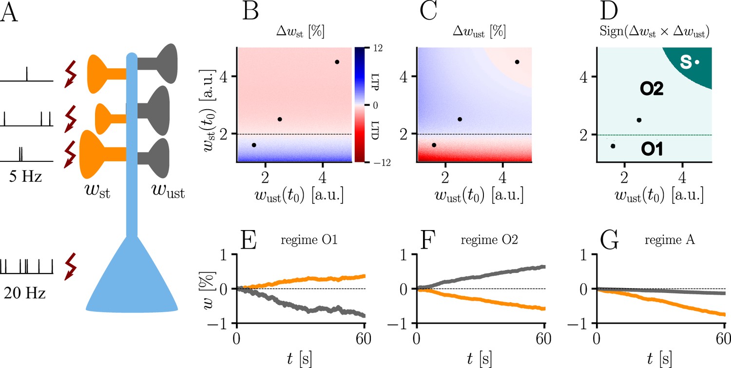
Interplay of homo- and heterosynaptic plasticity in natural-gradient learning.

(A) Simulation setup. Five out of 10 inputs received excitatory Poisson input at 5 Hz. In addition, we assumed the presence of tonic inhibition as a balancing mechanism for keeping the neuron’s output within a reasonable regime. Afferent stimulus was paired with teacher spike trains at 20 Hz and plasticity at both stimulated and unstimulated synapses was evaluated in comparison with their initial weights. For simplicity, initial weights within each group were assumed to be equal. (B) Weight change of stimulated weights (both homo- and heterosynaptic plasticity are present). These weight changes are independent of unstimulated weights. Equilibrium (dashed black line) is reached when the neuron’s output matches its teacher and the error vanishes. For increasing stimulated weights, potentiation switches to depression at the equilibrium line. (C) Weight change of unstimulated weights (only heterosynaptic plasticity is present). For very high activity caused by very large synaptic weights, heterosynaptic plasticity always causes synaptic depression. Otherwise, plasticity at unstimulated synapses behaves exactly opposite to plasticity at stimulated synapses. Increasing the size of initial stimulated weights results in a change from depression to potentiation at the same point where potentiation turns into depression at stimulated synapses. (D) Direct comparison of plasticity at stimulated and unstimulated synapses. The light green area (**O1, O2**) represents opposing signs, dark green (S) represents the same sign (more specifically, depression). Their shared equilibrium is marked by the dashed green line and represents the switch from positive to negative error. (**E–G**) Relative weight changes of synaptic weights for stimulated and unstimulated synapses during learning, with initial weights picked from the different regimes indicated by the crosses in (**B, C, D**).

Figure 8

Download asset Open asset

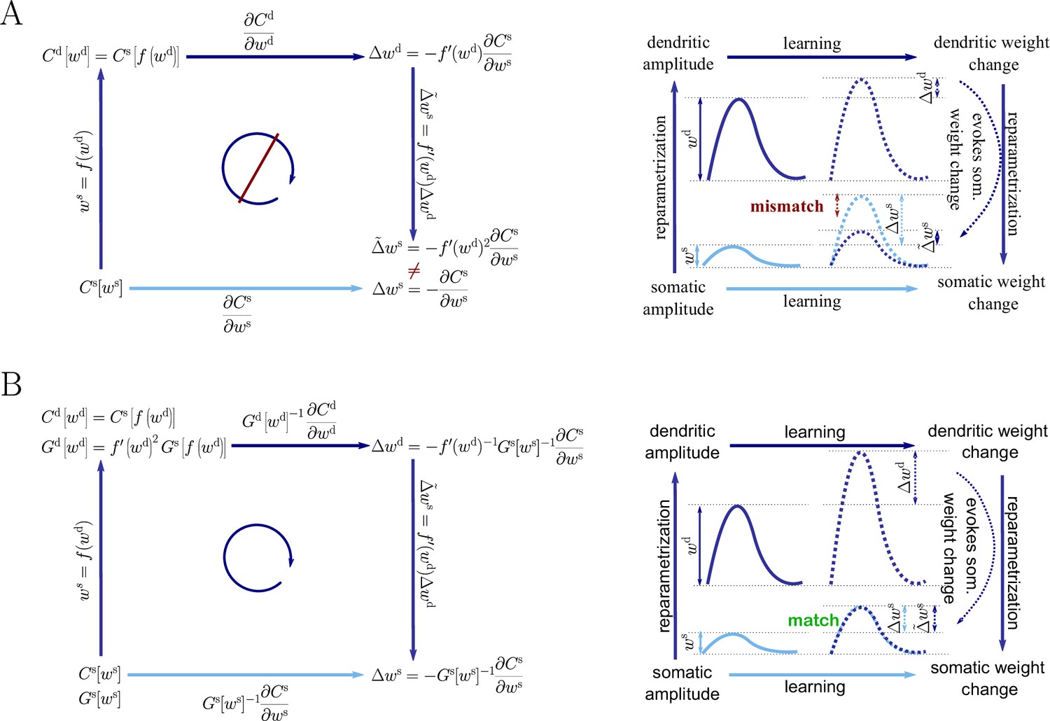
Natural-gradient descent does not depend on chosen parametrization.

Mathematical derivation and phenomenological correlates. EPSPs before learning are represented as continuous, after learning as dashed curves. The light blue arrow represents gradient descent on the error as a function of the somatic EPSP $C^{s} [w^{s}]$ (also shown in light blue). The resulting weight change leads to an increase $Δ w^{s}$ in the somatic EPSP after learning. The dark blue arrows track the calculation of the same gradient, but with respect to the dendritic EPSP (also shown in dark blue): (1) taking the attenuation into account in order to compute the error as a function of $w^{d}$ , (2) calculating the gradient, followed by (3) deriving the associated change in $\tilde{Δ} w^{s}$ , again considering attenuation. (A) For Euclidean-gradient descent. (B) For natural-gradient descent. Unlike for Euclidean-gradient descent, the factor $f^{'} (w)^{2}$ is compensated, since its inverse enters via the Fisher information. This leads to the synaptic weights updates, as well as the associated evolution of a neuron’s output statistics over time, being equal under the two parametrizations.

Figure 9

Download asset Open asset

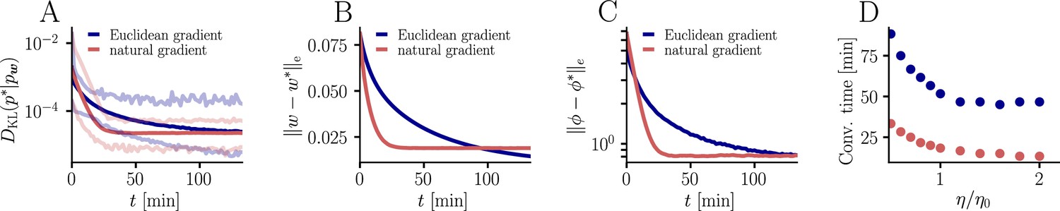
Further convergence analysis of natural-gradient-descent learning.

Unless stated otherwise, all simulation parameters are the same as in Figure 3. (A) In addition to the average learning curves from Figure 3F (solid lines), we show the minimum and maximum values (semi-transparent lines) during learning. (B) Plot of the mean Euclidean distance between student and teacher weight. Note that a smaller distance in weights does not imply a smaller $D_{KL}$ , nor a smaller distance in firing rates. This is due to the non-linear relationship between weights and firing rates. (C) Development of mean Euclidean distance between student and teacher firing rate during learning. (D) Robustness of learning against perturbations of the firing rate. We varied the learning rate for natural-gradient and Euclidean-gradient descent relative to the learning rate $η_{0}$ used in the simulations for Figure 3F (EGD: $η_{0} = η_{e} = 4.5 * 10^{- 7}$ , NGD: $η_{0} = η_{n} = 6 * 10^{- 4}$ ), and measured the time until the $D_{KL}$ first reached a value of $5 * 10^{- 5}$ .

Figure 10

Download asset Open asset

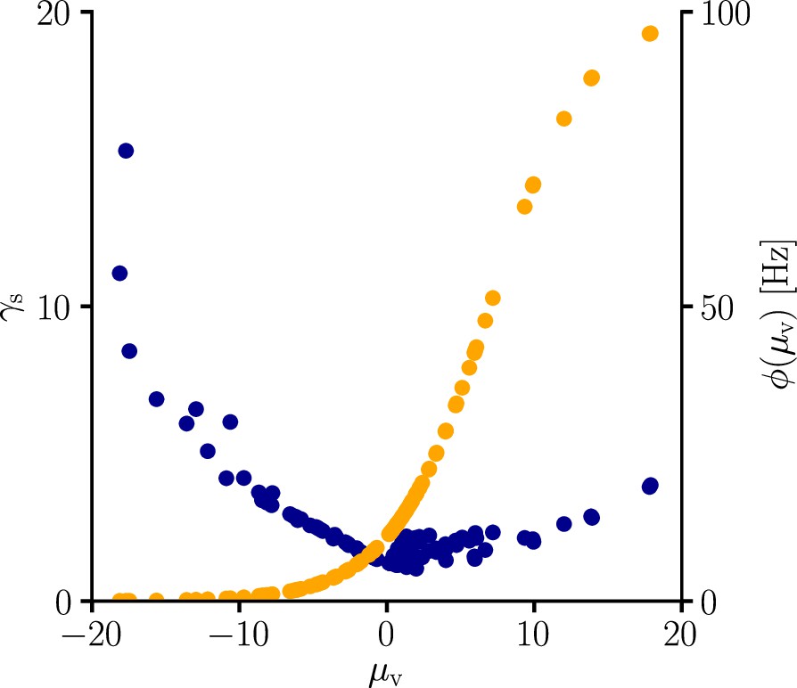
Global learning rate scaling $γ_{s}$ as a function of the mean membrane potential.

We sampled the global learning rate factor $γ_{s}$ (blue) for various conditions. In line with Equation 107, $γ_{s}$ is boosted in regions where the transfer function is flat, that is, $ϕ^{'} (V)$ is small. The global scaling factor is additionally increased in regions where the transfer function reaches high absolute values.

Figure 11

Download asset Open asset

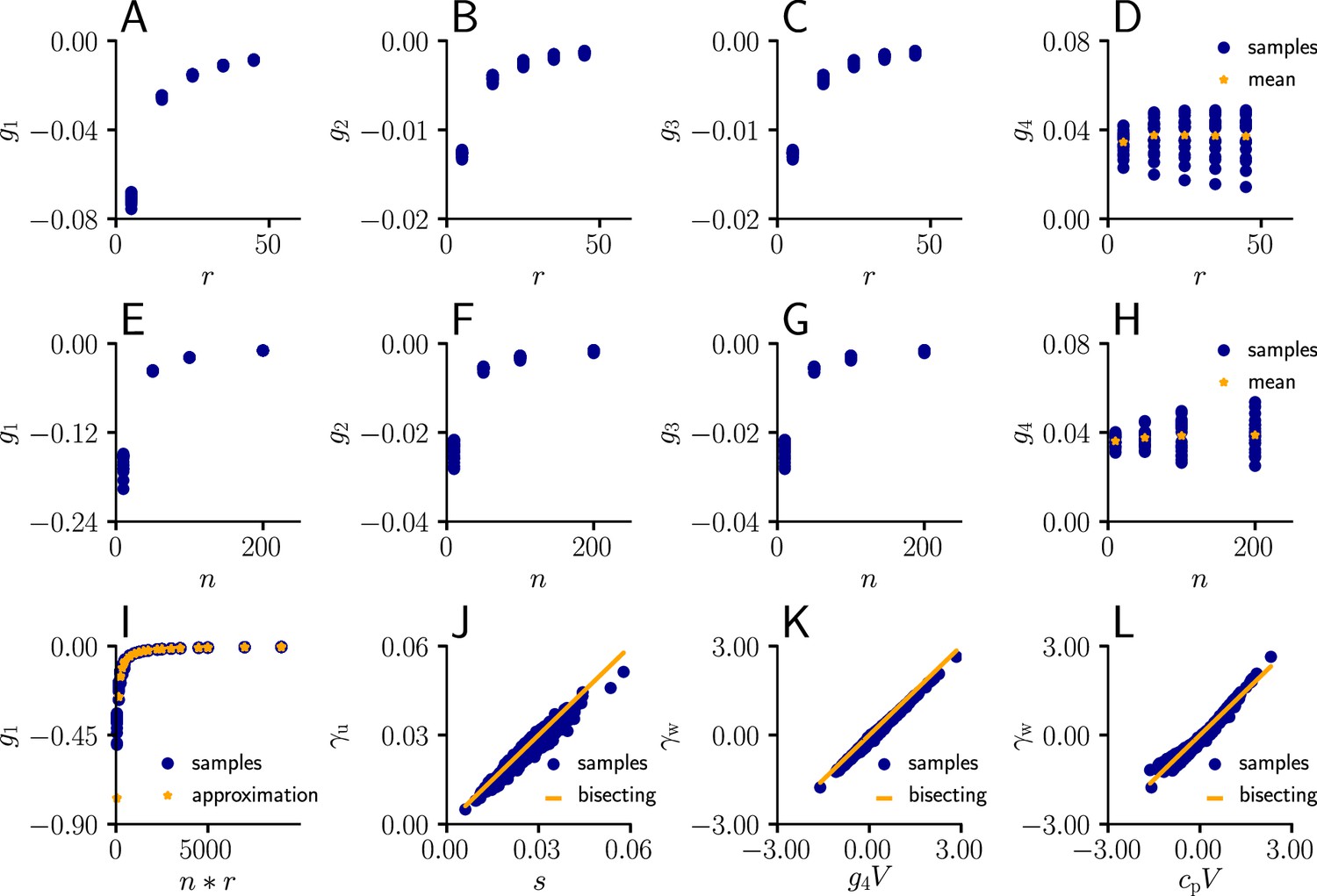
Learning rule coefficients can be approximated by simpler quantities.

(A)-(D) Samples values for $g_{1}, \dots, g_{4}$ for different afferent input rates. (E)-(H) In a second simulation, we varied the number $n$ of afferent inputs. (I) Comparison of the sampled values of $g_{1}$ (blue) as a function of the total input rate $n * r$ to the values of the approximation given by $g_{1} \approx - q^{- 1}$ . (J) Sampled values of $γ_{u}$ (blue) as a function of the approximation s (Equation 111). The proximity of the sampled values to the diagonal indicates that $s$ may indeed serve as an approximation for $γ_{u}$ . (K) Sampled values of $γ_{w}$ (blue) as a function of $g_{4} V$ . The proximity of the sampled values to the diagonal indicates that $g_{4} V$ serves as an approximation for $γ_{w}$ . (L) Same as (K), but with $g_{4}$ replaced by a constant $c_{w} = 0.05$ .

Figure 12

Download asset Open asset

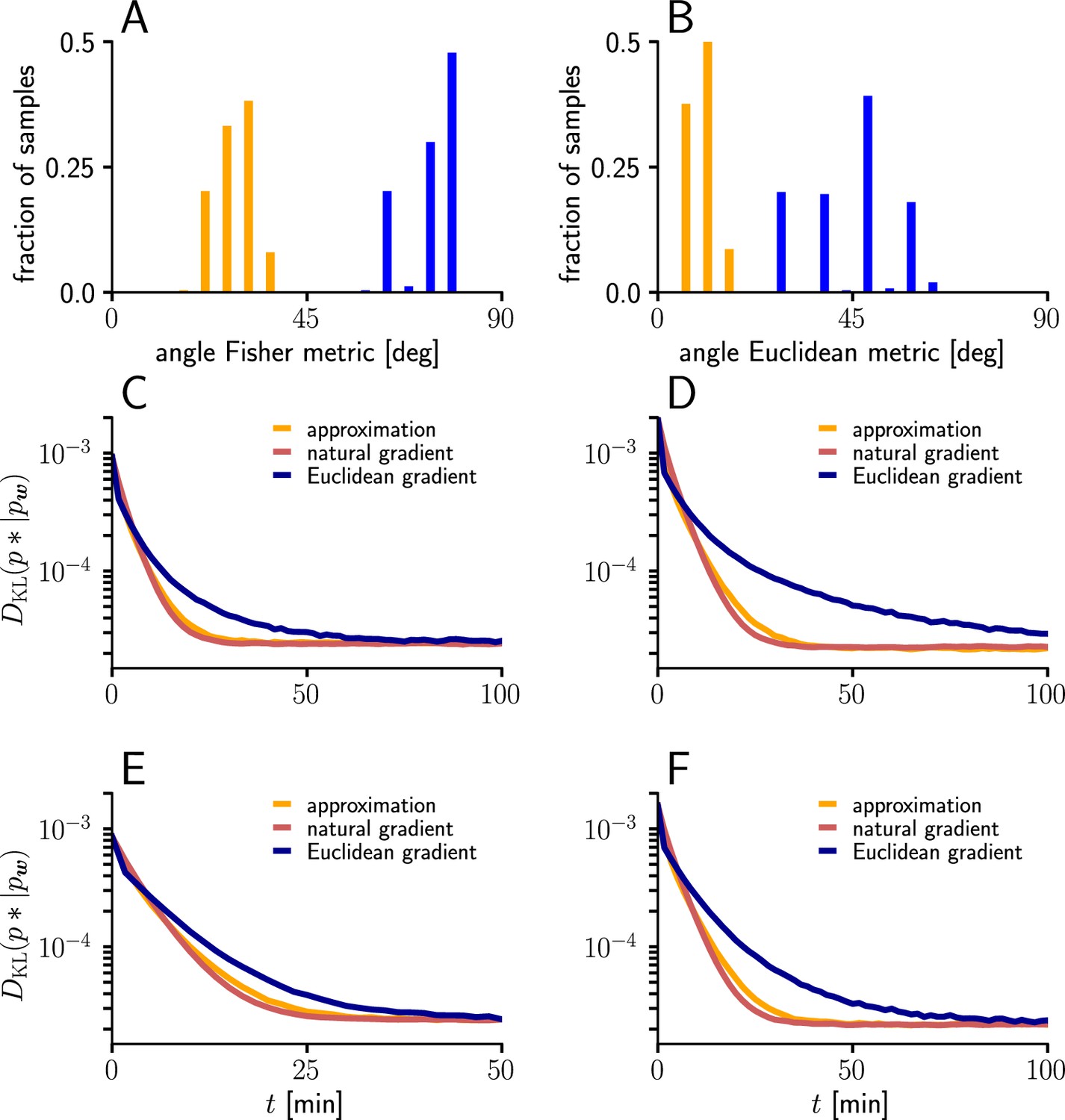
Natural-gradient learning can be approximated by a simpler rule in many scenarios.

(A) Mean Fisher angles between true and approximated weight updates (orange) and between natural and Euclidean weight updates (blue), for $n = 100$ . Results for several input patterns were pooled (group1/group2: 10 Hz/10 Hz 10 Hz/30 Hz, 10 Hz/50 Hz, 20 Hz/20 Hz, 20 Hz/40 Hz). Initial weights and input spikes were sampled randomly (100 randomly sampled initial weight vectors per input pattern; for each, angles were averaged over 100 input spike train samples per afferent). (B) Same as (A), but angles measured in the Euclidean metric. (**C–F**) Comparison of learning curves for natural gradient (red), Euclidean gradient (blue) and approximation (orange) for $n = 100$ afferents. Simulations were performed in the setting of Figure 3, under multiple input conditions. (C) Group one firing with 10 Hz, group two firing at 30 Hz. (D) Group one firing with 10 Hz, group two firing at 50 Hz. (E) Group one firing with 20 Hz, group two firing at 20 Hz. (F) Group one firing with 20 Hz, group two firing at 40 Hz.

Tables

Table 1

Learning rates.

r₁	r₂	$η_{n}$	$η_{a}$	$η_{e}$
10 Hz	30 Hz	0.000655	0.00055	0.00000110
10 Hz	50 Hz	0.000600	0.00045	0.00000045
20 Hz	20 Hz	0.000650	0.00053	0.00000118
20 Hz	40 Hz	0.000580	0.00045	0.00000055

Additional files

Transparent reporting form: https://cdn.elifesciences.org/articles/66526/elife-66526-transrepform1-v1.docx
Download elife-66526-transrepform1-v1.docx
Source data 1 Source data for figures.: https://cdn.elifesciences.org/articles/66526/elife-66526-data1-v1.zip
Download elife-66526-data1-v1.zip

Download links

A two-part list of links to download the article, or parts of the article, in various formats.

Downloads (link to download the article as PDF)

Article PDF

Open citations (links to open the citations from this article in various online reference manager services)

Mendeley

Cite this article (links to download the citations from this article in formats compatible with various reference manager tools)

Elena Kreutzer
Walter Senn
Mihai A Petrovici

(2022)

Natural-gradient learning for spiking neurons

eLife 11:e66526.

https://doi.org/10.7554/eLife.66526

Share this article

Cite this article

Classical gradient descent depends on chosen parametrization.

The natural gradient represents the true gradient direction on the manifold of neuronal input-output distributions.

Natural-gradient plasticity speeds up learning in a simple regression task.

Natural-gradient learning scales synaptic weight updates depending on their distance from the soma.

Natural-gradient learning scales approximately inversely with input variance.

Natural-gradient learning combines multiple forms of plasticity.

Interplay of homo- and heterosynaptic plasticity in natural-gradient learning.

Natural-gradient descent does not depend on chosen parametrization.

Further convergence analysis of natural-gradient-descent learning.

Global learning rate scaling γs as a function of the mean membrane potential.

Learning rule coefficients can be approximated by simpler quantities.

Natural-gradient learning can be approximated by a simpler rule in many scenarios.

Learning rates.

Transparent reporting form

Source data 1

Downloads (link to download the article as PDF)

Open citations (links to open the citations from this article in various online reference manager services)

Cite this article (links to download the citations from this article in formats compatible with various reference manager tools)

Global learning rate scaling $γ_{s}$ as a function of the mean membrane potential.