Figures and data in Polygenic adaptation after a sudden change in environment

Version of Record

Accepted for publication after peer review and revision.

Download
Cite
Share
CommentOpen annotations (there are currently 0 annotations on this page).

Version of Record published: November 23, 2022 (This version)
Accepted Manuscript updated: September 27, 2022 (Go to version)
Accepted Manuscript published: September 26, 2022 (Go to version)
Accepted: July 18, 2022
Received: January 19, 2021
Preprint posted: October 3, 2019 (Go to version)

Figures
Tables
Additional files

39 figures, 2 tables and 1 additional file

Figures

Figure 1

Download asset Open asset

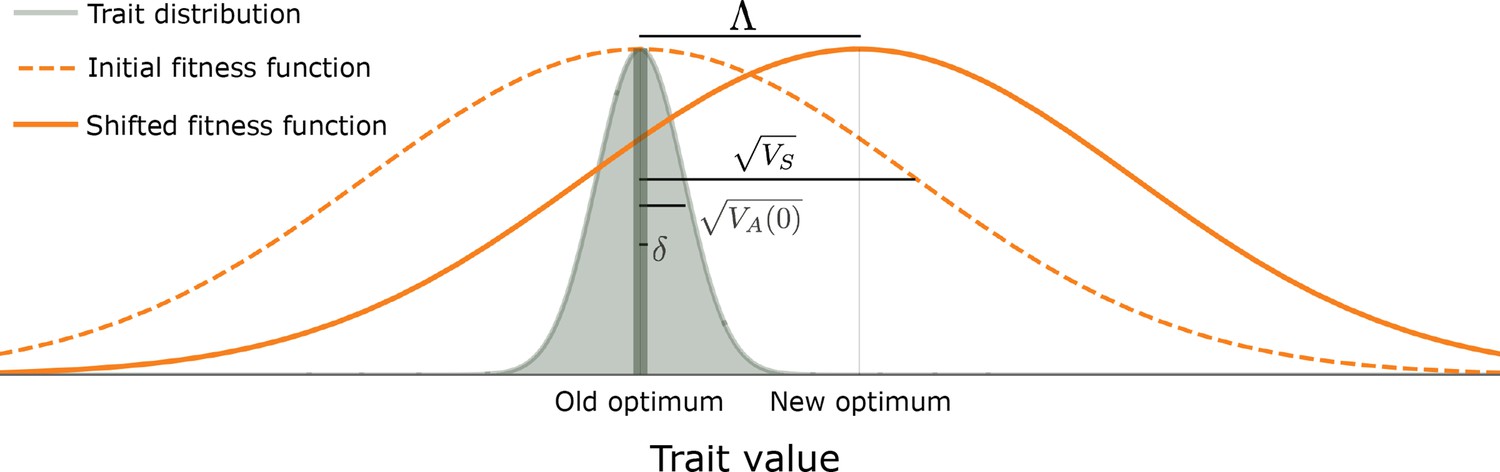
The evolutionary scenario.

Before the shift in optimum, phenotypes are distributed symmetrically, with a mean that is very close to the old optimum and a standard deviation that is substantially smaller than the width of the fitness function ( $V_{A} (0) ≪ V_{S}$ ). We consider the response to an instantaneous shift in optimum, for the case where the magnitude of the shift is smaller than the width of the fitness function ( $Λ ⪅ \sqrt{V_{S}}$ ). See text for further details.

Figure 2

Download asset Open asset

The phenotypic response to a shift in optimal phenotype.

(A) Cartoon of the two kinds of phenotypic response: (i) the Lande approximation, in which the mean approaches the new optimum exponentially with time and the phenotypic distribution maintains its shape; (ii) substantial deviations from Lande’s approximation, in which the mean approaches the new optimum rapidly at first, but during this time the phenotypic distribution becomes skewed, causing the mean’s approach to slow down dramatically, to a rate that is dictated by the decay of the 3^rd central moment. (B) In both the Lande and non-Lande cases, the mean phenotype initially approaches the new optimum rapidly. This approach is described by Lande’s approximation, and is thus almost identical in the two cases (which is why only the Lande curve is visible). The simulation results were generated using the *all alleles* simulation with a shift of $Λ = 4 \cdot \sqrt{V_{A} (0)}$ , as detailed in *Simulations and resources*. For each quantity described in **B-D**, we show the simulations’ mean ±1.96 SE (solid lines and shaded regions, respectively). (C) In the non-Lande case, the phenotypic variance and skewness increase during the rapid phase and then take a very long time to decay to their values at equilibrium. (D) Over the longer-term, the approach to the optimum in the non-Lande case almost grinds to a halt, where its rate can be described by the quasi-static approximation (Equation 6). While the non-Lande response differs from Lande’s approximation, the difference is small: the maximal deviation in mean phenotype is $\sim 0.06 \cdot \sqrt{V_{A} (0)}$ , the variance increases by ∼ 10% and the maximal skewness is tiny (less than 0.01).

Figure 3

Download asset Open asset

A cartoon of allele dynamics.

We divide the allele dynamics into rapid and equilibration phases, based on the rate of phenotypic change, and consider the trajectories of alleles with opposing effects of the same magnitude, which start at the same initial minor frequency. During the rapid phase, alleles whose effects align with the shift slightly increase in frequency relative to those with opposing effects. During the equilibration phase, this frequency difference can increase further and eventually leads aligned alleles to fix with slightly greater probabilities than opposing ones.

Figure 4

Download asset Open asset

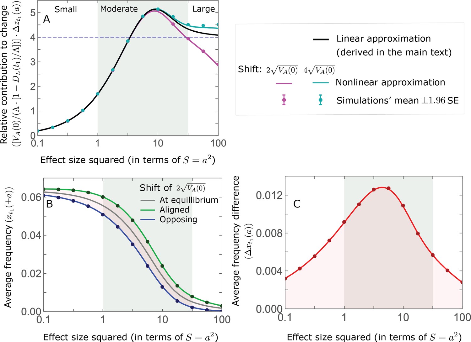
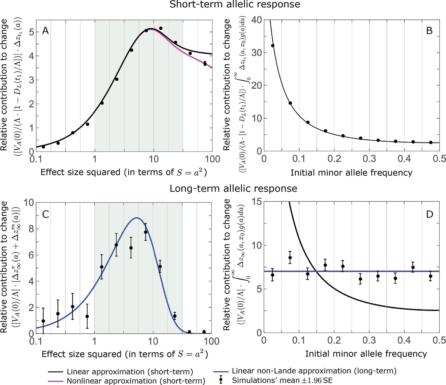
The allelic response during the rapid phase.

(A) Alleles with moderate and large magnitudes make the greatest contribution to phenotypic change (per unit mutational input). The results of our linear approximation (derived in the main text) are compared with a more accurate nonlinear one (derived in Section 4.1.2 of *Appendix 3*) and with simulations. (B) The average MAF of aligned and opposing alleles at the end of the rapid phase decreases with effect size squared. (C) The expected frequency difference between pairs of opposing alleles is greatest for moderate effect sizes. In B and C, the results of the nonlinear approximation are compared with simulations. The simulation results in all panels were were generated using the *single allele* simulation, as detailed in *Simulations and resources*; error bars are not visible because they are smaller than the points.

Figure 5

Download asset Open asset

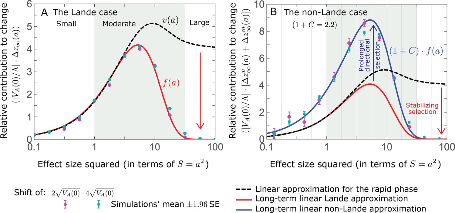
The long-term (fixed) allelic contribution to phenotypic adaptation.

We show the relative contribution of alleles as a function of effect size squared, based on the linear approximations and on simulations with the two shift sizes specified in the caption. (A) The Lande case. The theoretical prediction is described by the function $f (a)$ (Equations 13 and 20), and simulation results were generated using the *single allele* simulation, as detailed in *Simulations and resources*; error bars are not visible because they are smaller than the points. Our prediction for the long-term contribution (corresponding to $f (a)$ ) is always below the prediction for the rapid phase (corresponding to $v (a)$ ). The difference becomes substantial for $a^{2} ⪆ 4$ , implying that the linear Lande approximation underestimates the fixed contribution when large effect alleles contribute markedly to the genetic variance at equilibrium. (B) The non-Lande case. Here, we assume an exponential distribution of effect sizes squared with $E (a^{2}) = 16$ , which yields an amplification factor of $1 + C \approx 2.2$ (Equation 22). The theoretical prediction for the joint contribution of standing variation and new mutations is described by the function $(1 + C) \cdot f (a) Λ / V_{A} (0)$ (Equation 28). Simulation results were generated using the *all alleles* simulation for the non-Lande case (see section on *Simulations and resources*). Specifically, we calculated the relative contribution of alleles in each effect size bin (between the gray gridlines), by dividing the contribution of all fixations in the bin by the mutation rate per generation corresponding to that bin. In both Lande and non-Lande cases, long-term stabilizing selection diminishes the contribution of alleles with large effects (red arrows). In the non-Lande case, long-term, weak directional selection greatly amplifies the contribution of alleles with small and moderate effects (blue arrow). See Appendix 3—figures 12–19 for other attributes of the long-term allelic response and for the nonlinear approximations.

Figure 6

Download asset Open asset

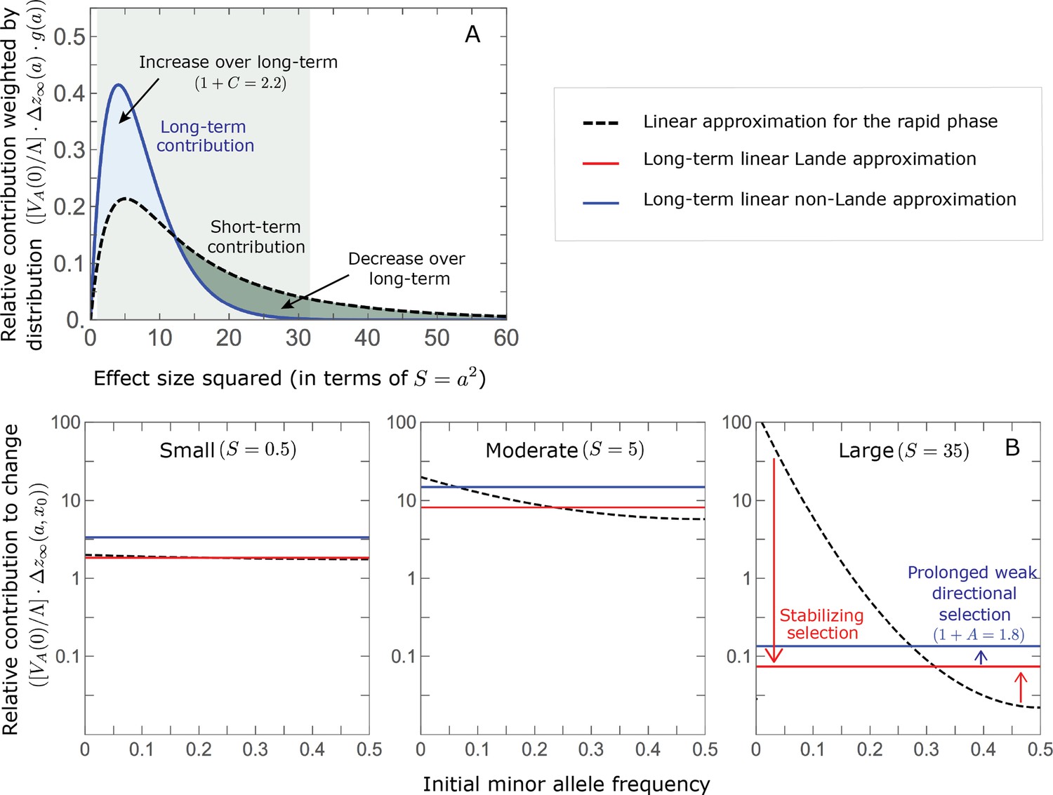
The genetic basis of adaptation turns over during the equilibration phase.

(A) The short-term contribution of large effect alleles is supplanted by the contribution of moderate effect alleles. As an illustration, we show the results of the linear approximation for the non-Lande case in Figure 5B (Equations 13 and 28). Specifically, we weight the short- and long-term relative contributions by the density of effect size squared (given $E (a^{2}) = 16$ ) and use a linear (rather than log) scale for the effect sizes squared. This way we can see that the decrease in the contribution of large effect alleles (shaded dark gray area) equals the increase in the contribution of moderate effect alleles (shaded blue area). (B) The proportional long-term contribution of alleles that segregated at low MAFs before the shift is diminished relative to their short-term contribution, an effect most pronounced for large effect sizes. As an illustration, we show the linear approximations for the contribution of alleles with a given effect size as a function of their initial MAF (Equations 12, 19 and 24) for the same non-Lande case as in A, with a shift of $Λ = 2 \sqrt{V_{A} (0)}$ . To this end, we estimate the amplification factor for standing variation ( $1 + A$ ) using *all alleles* simulations for the non-Lande case (see section on *Simulations and resources* and Section 5.2 of *Appendix 3*). In both the Lande and non-Lande cases, long-term stabilizing selection diminishes the contribution of alleles with lower initial MAF and amplifies the contribution of alleles with higher initial MAF (red arrows). In the non-Lande case, prolonged, weak directional selection amplifies the contribution of alleles, regardless of their initial MAF (blue arrow).

Figure 7

Download asset Open asset

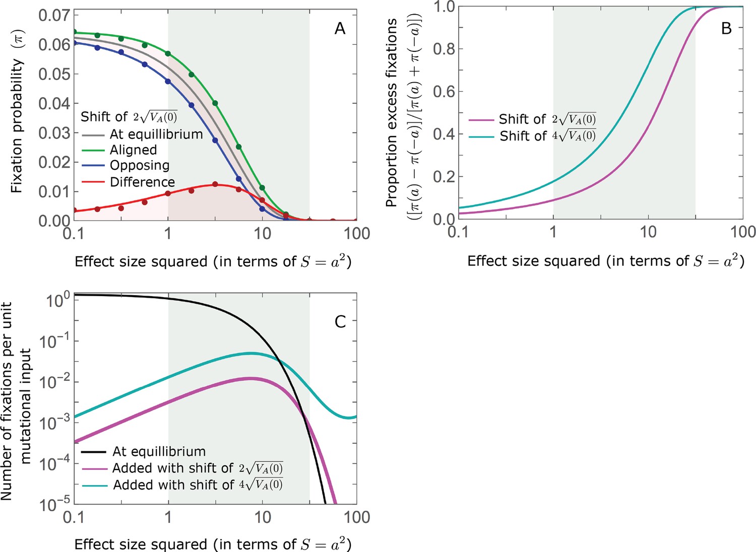
While long-term phenotypic adaptation arises from an excess in fixations of aligned relative to opposing alleles, this excess and its effect on the total number of fixations is typically small.

(A) The fixation probabilities of aligned and opposing alleles segregating before the shift, as a function of their effect size squared. Simulation results were generated using the *single alleles* simulation, as detailed in *Simulations and resources*; error bars are not visible because they are smaller than the points. Analytic predictions in all panels were calculated using the nonlinear Lande approximation derived in Section 5.3 of *Appendix 3*. For large effect sizes, the fixation probabilities become vanishingly small, whereas for small and moderate effect sizes, the difference in the fixation probabilities of alleles with opposing effects is small. (B) The relative excess of fixations of aligned alleles as a function of effect size squared. (C) Polygenic adaptation typically adds a small number of fixations relative to the number at equilibrium. For large effect sizes, the relative increase in number is large, but their absolute number and the corresponding contribution to phenotypic adaptation are extremely small.

Figure 8

Download asset Open asset

Equilibrium around the new optimum is restored on a time scale of $2 N$ generations after the shift.

The change in fixed distance after the shift estimated using *all alleles* simulations for the Lande and non-Lande cases (see section on *Simulations and resources*) is compared with an exponential decay with a rate of $1 / (2 N)$ per generation. See Appendix 3—figure 28 for similar comparisons using a broad range of model parameter values.

Appendix 2—figure 1

Download asset Open asset

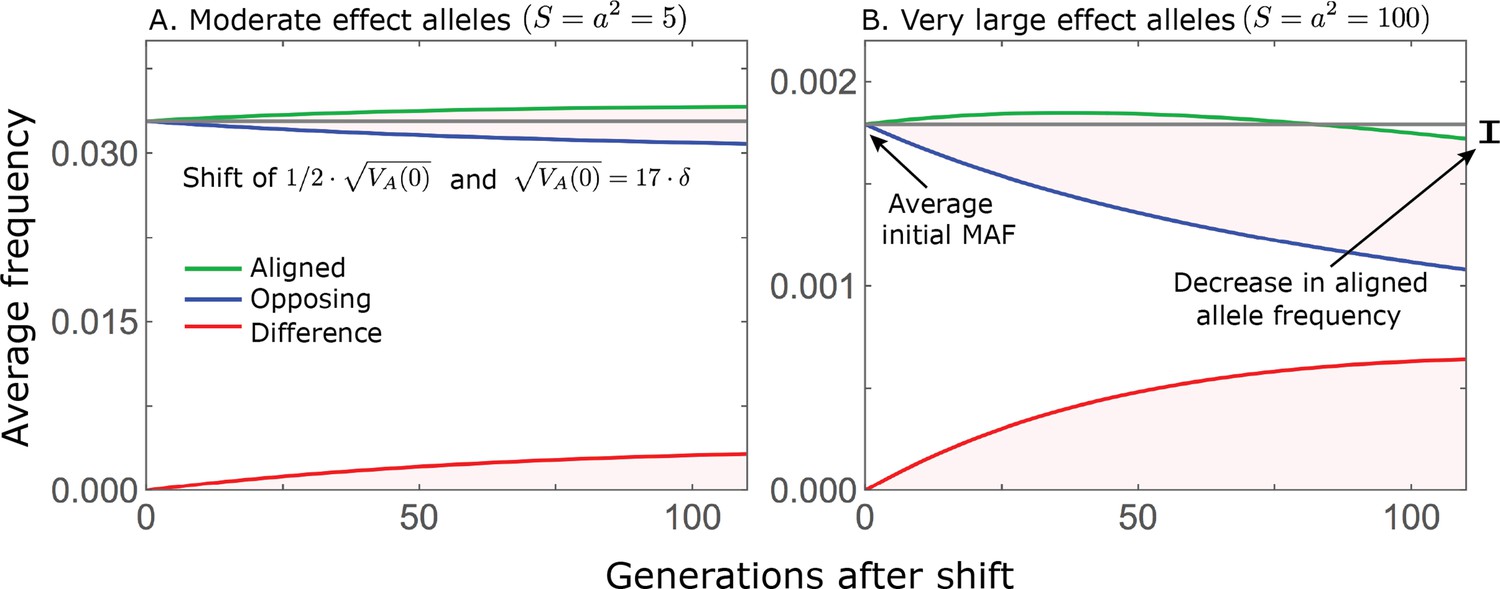
While directional selection during the rapid phase increases the frequency of aligned alleles relative to opposing ones, the frequency of aligned alleles does not necessarily increase.

Here, we show an example of the trajectories of (A) moderate and (B) large effect alleles in response to a relatively small shift in optimum; the trajectories were calculated using Equations A3-39, A3-40 and A3-48 in *Appendix 3*. When directional selection is sufficiently weak (the shift is small), the frequency of aligned alleles with sufficiently large effects will decrease (B). However, the frequency of opposing alleles decreases *more*, and the frequency difference (in red) contributes to the change in mean phenotype.

Appendix 2—figure 2

Download asset Open asset

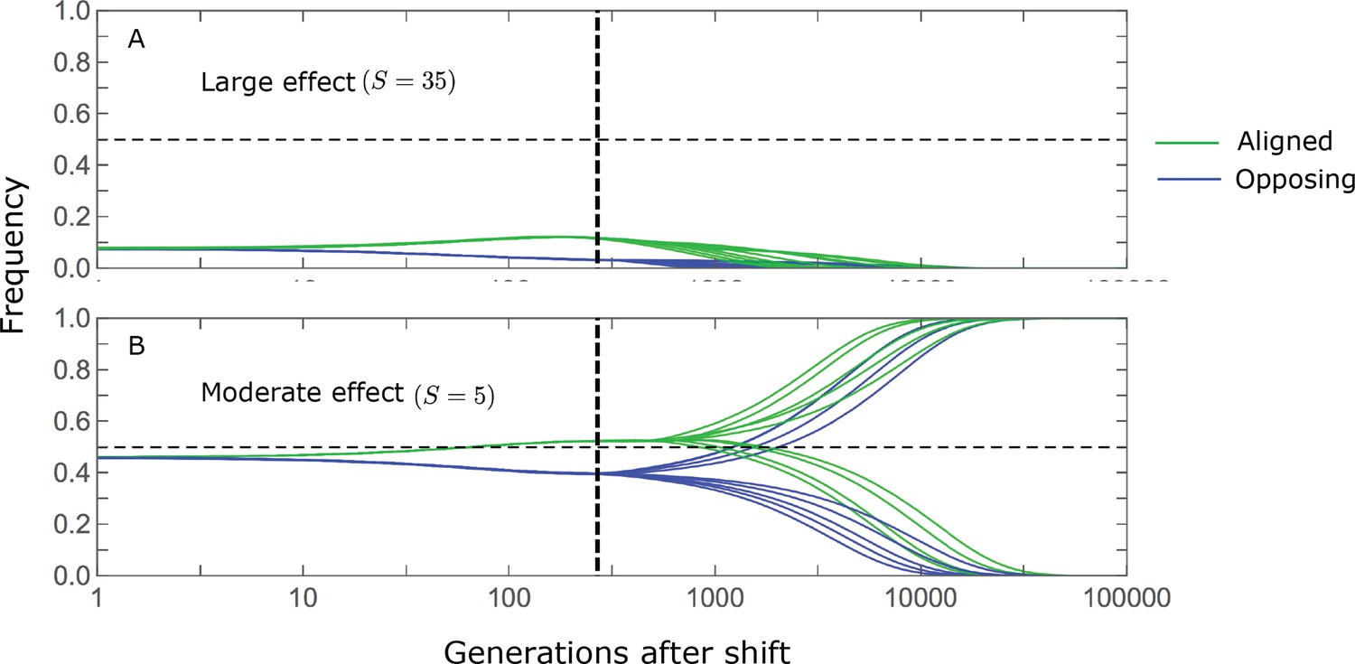
Stabilizing selection during the equilibration phase causes turnover in the genetic basis of adaptation.

The cartoons depict the trajectories of alleles with opposing effects of given magnitudes and initial MAFs. For the purpose of illustration, we focus on alleles with large (A) and moderate (B) effects, with initial MAFs in the tail of the corresponding equilibrium MAF distribution (the 99.5^th percentile), and a shift size of $Λ = 2 \cdot \sqrt{V_{A} (0)}$ with $\sqrt{V_{A} (0)} = 17 δ$ . Directional selection during the rapid phase increases the frequency of aligned alleles relative to those with opposing effects, and these frequency differences underlie short-term phenotypic adaptation. (A) The initial MAF of large effect alleles, even those in the 99.5^th percentile, is sufficiently low such that both aligned and opposing alleles still have low MAFs at the end of the rapid phase. Consequently, they are both strongly selected against during the equilibration phase and almost certainly go extinct, thereby erasing their short-term contribution to phenotypic adaptation. (B) Moderate effect alleles start at much higher initial MAFs. In the extreme, this initial frequency is sufficiently high for directional selection during the rapid phase to push aligned alleles above frequency 1/2, thereby reversing the direction of (under-dominant) selection on them, but not on the opposing alleles, during the equilibration phase. Consequently, the expected contribution of moderate effect alleles with sufficiently high initial MAF to phenotypic adaptation is amplified during the equilibration phase.

Appendix 2—figure 3

Download asset Open asset

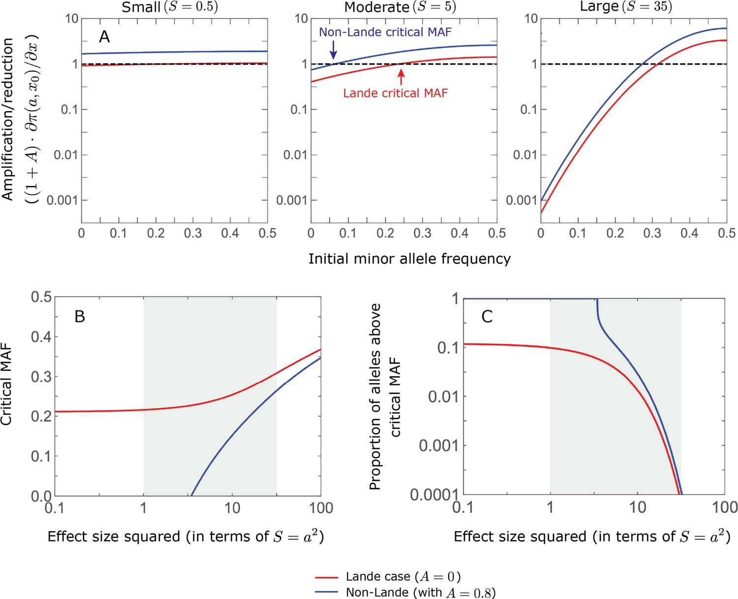
The long-term phenotypic contribution of minor alleles is amplified if they start above a critical initial frequency, which depends on their magnitude, and it is diminished if they start below this critical MAF.

In the linear approximation, we found that
$Δ z_{\infty} (a, x_{0}) \approx (1 + A) \cdot Δ z_{\infty}^{L} (a, x_{0}) = (1 + A) \cdot \partial π / \partial x (a, x_{0}) \cdot Δ z_{d}^{L} (a, x_{0})$
(Equation 24 in the main text). Further assuming that $Δ z_{t_{1}} (a, x_{0}) \approx Δ z_{d}^{L} (a, x_{0})$ (which holds if the shift is not miniscule, that is, $Λ ≫ δ$ ), we find that the (multiplicative) amplification/reduction of the phenotypic contribution is approximated by $(1 + A) \cdot \partial π / \partial x (a, x_{0})$ . In this approximation, the critical MAF for alleles with magnitude satisfies
$(1 + A) \cdot \partial π / \partial x (a, x_{c}) = 1.$
(A) The amplification/reduction for alleles with small (left), moderate (middle), and large (right) effects as a function of initial MAF, in the Lande (red) and non-Lande (blue) case. The curves and critical MAFs are calculated from the above equations. Given a factor $A > 0$ , the contribution of alleles with sufficiently small effect sizes are amplified for any initial MAF $x_{0}$ (Figure 6), because $\partial π / \partial x (a, x_{0}) \approx 1$ and thus $Δ z_{\infty}^{L} (a, x_{0}) \approx Δ z_{d}^{L} (a, x_{0})$ and $Δ z_{\infty}^{v} (a, x_{0}) > Δ z_{t_{1}} (a, x_{0})$ . In turn, for sufficiently large effect sizes, the curves for $Δ z_{\infty}^{v} (a, x_{0})$ and $Δ z_{d}^{L} (a, x_{0})$ ( $\approx Δ z_{t_{1}} (a, x_{0})$ ) intersect (Figure 6B) and thus a critical MAF exists (i.e., $0 < x_{c} < 1 / 2$ ). These considerations explain why, for sufficiently large effect sizes, the long-term contribution of alleles with low initial MAFs is diminished relative to their short-term contribution. (B) The critical MAF as a function of effect size in the Lande and non-Lande case (based on $(1 + A) \cdot \partial π / \partial x (a, x_{c}) = 1$ ). The critical MAF is lower in the non-Lande case, because $A > 0$ . This proportion declined with increasing allele magnitude both because initial MAFs at equilibrium decrease and because the critical MAF increases (panel B). It is greater in the non-Lande case because the critical MAF is lower (panel B). (C) The proportion of segregating sites at equilibrium with MAF exceeding the critical MAF.

Appendix 3—figure 1

Download asset Open asset

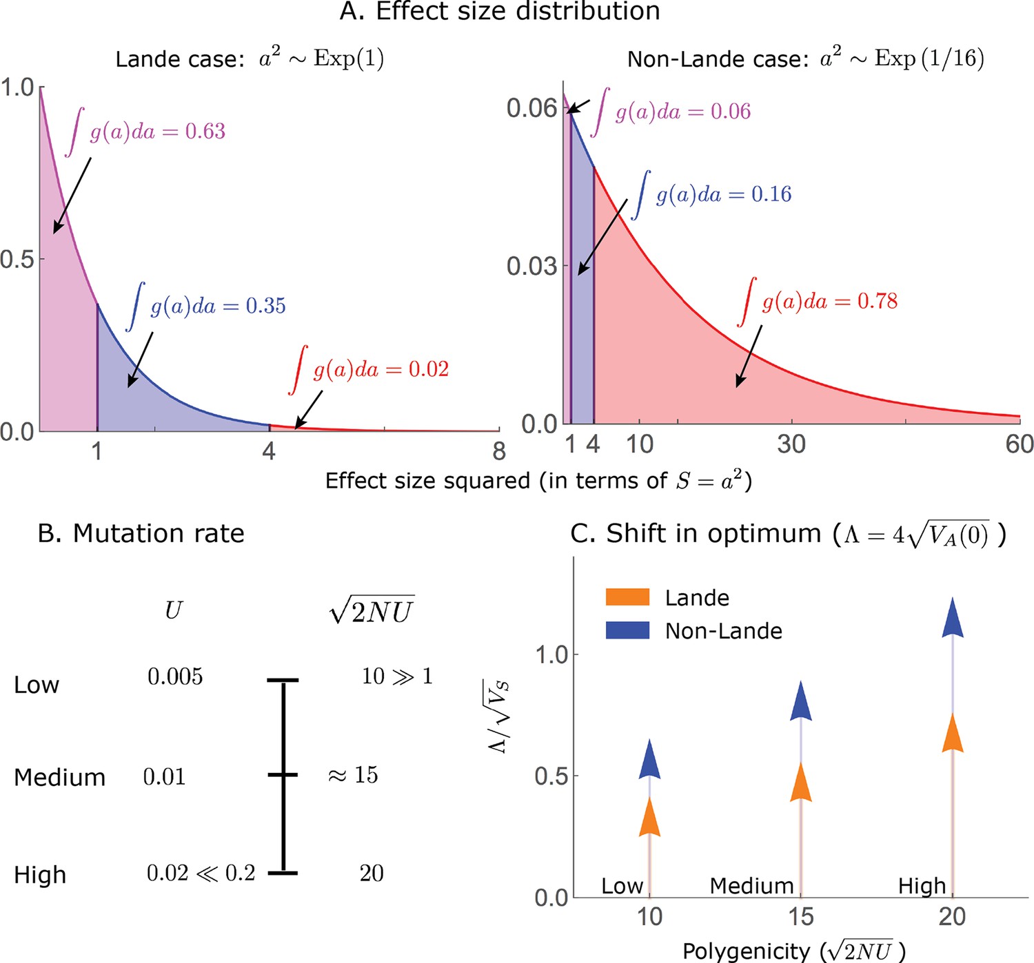
Our simulation parameter values are chosen to span as wide a range as possible given our conditions on them.

Appendix 3—figure 2

Download asset Open asset

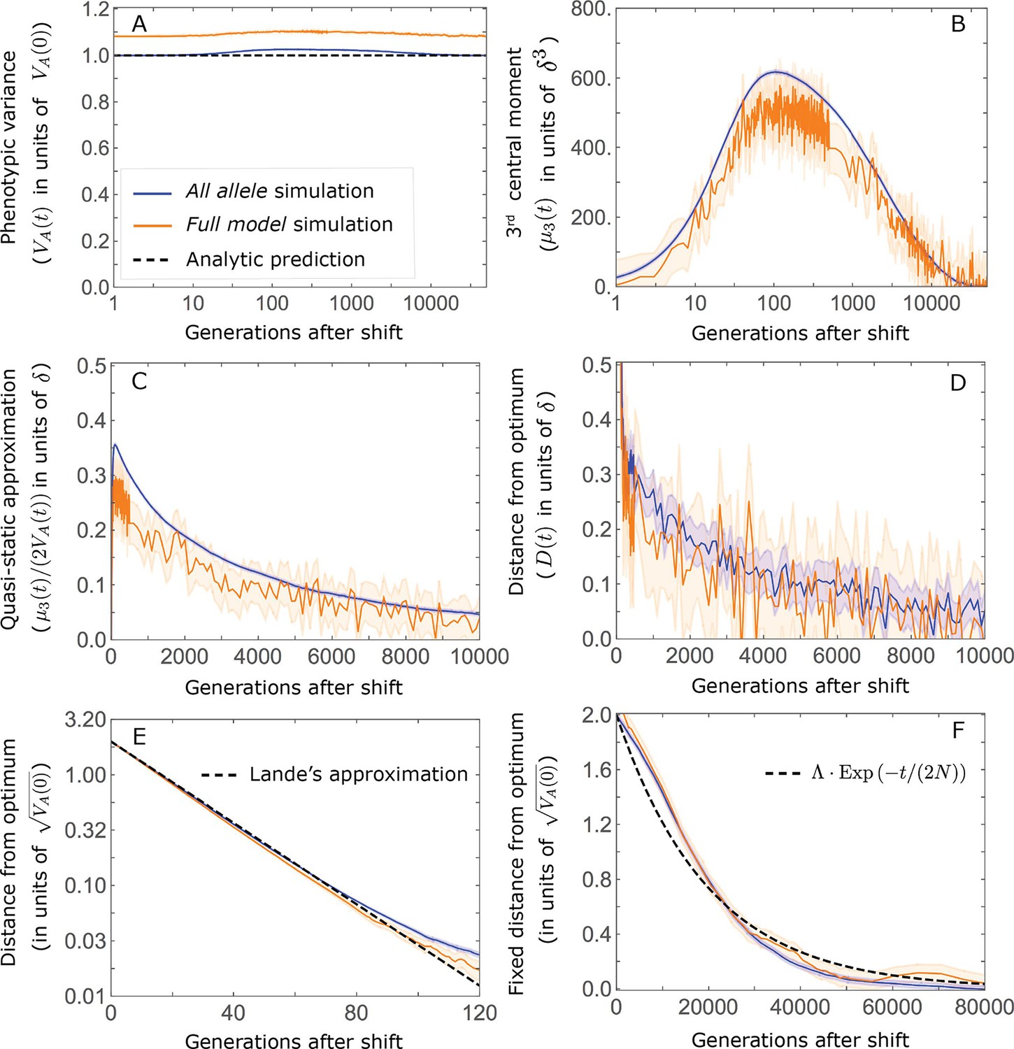
Comparison of our main results about the phenotypic dynamics with corresponding results from the *full model* simulations.

The results shown are based on 2500 *all alleles* and 500 *full model* simulations with the parameters of the non-Lande case used in the main text (see section on *Simulations and resources*), i.e. $N = 10^{4}$ , $U = 0.01$ , an exponential distribution of effect sizes squared with $E (a^{2}) = 16$ , which together imply $\sqrt{V_{A} (0)} = 29 \cdot δ$ , and a shift size of $Λ = 2 \cdot \sqrt{V_{A} (0)}$ . (A) Phenotypic variance. (B) 3^rd phenotypic moment. (C) The quasi-static approximation for the mean phenotypic distance from optimum ( $μ_{3} (t) / (2 V_{A} (t))$ ; Equation A3-6 in the main text). (D) The mean phenotypic distance from optimum. (E) The mean phenotypic distance from optimum shortly after the shift (during the rapid phenotypic response). (F) The fixed distance from the optimum (defined in the section on *Other properties of the equilibration process*).

Appendix 3—figure 3

Download asset Open asset

Comparison of our main results about the allele dynamics with the corresponding results of the *full model* simulations.

The results shown are based on 500 *full model* simulations with the parameters of the non-Lande case used in the main text (see section on *Simulations and resources*). We calculate the relative contribution from each effect size bin (between the gray gridlines) by dividing the contribution of all alleles in the bin by the mutation rate per generation corresponding to that bin. We show the relative phenotypic contribution per unit mutational input of alleles as a function of effect size squared (A and C) and initial MAF (B and D) in the rapid (top) and equilibration (bottom) phases.

Appendix 3—figure 4

Download asset Open asset

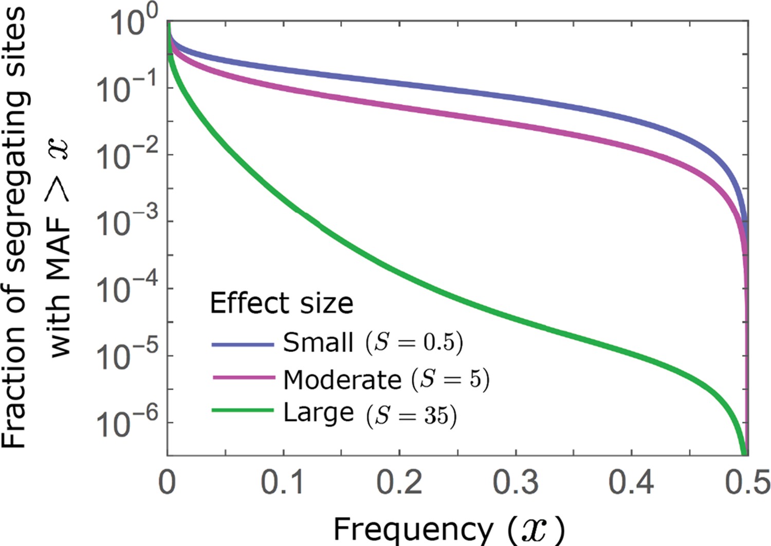
Allelic densities at equilibrium.

We show the proportion of segregating sites with MAF $> x$ as a function of $x$ . Minor alleles segregate at much lower frequencies at sites with larger effects than at sites with intermediate and small effects (see Equations A3-22 and A3-27).

Appendix 3—figure 5

Download asset Open asset

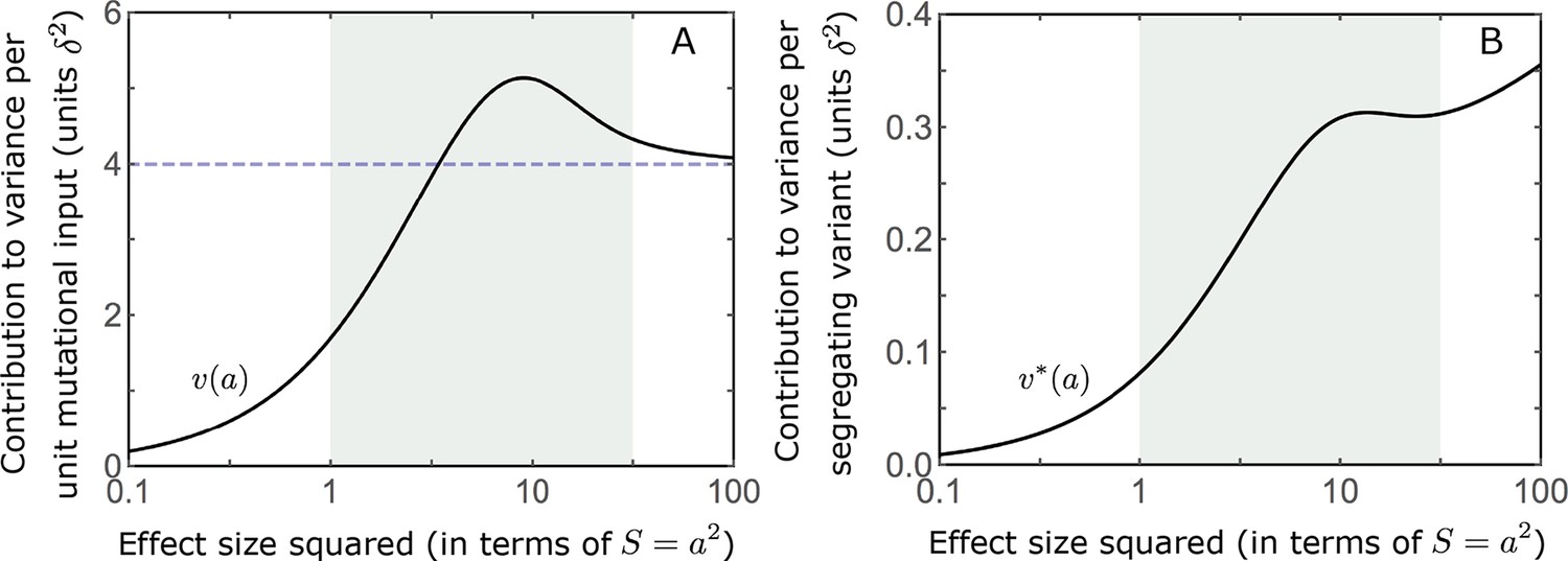
The distribution of variance at equilibrium.

We show the contribution to variance per unit mutational input (A) (based on Equation A3-29) and per segregating variant (B) as a function of effect size squared.

Appendix 3—figure 6

Download asset Open asset

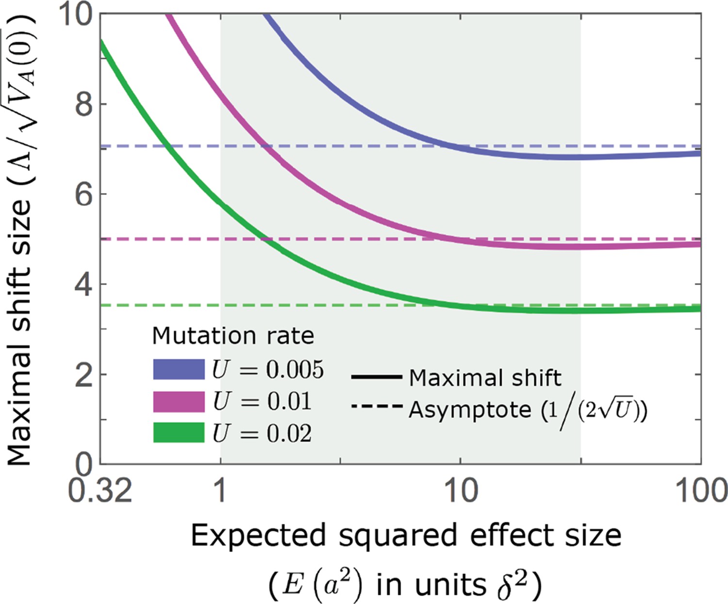
An upper bound on shift size measured in phenotypic standard deviations.

As detailed in the text, our condition that $Λ ⪅ \sqrt{V_{S}}$ sets an upper bound on $Λ / \sqrt{V_{A} (0)}$ , which in turn depends on the mutation rate $U$ and the distribution of effect sizes (Equation A3-31). As an illustration, we assume an exponential distribution of effect sizes squared, with the expectation $E (S) = E (a^{2})$ shown on the $x$ -axis; the $x$ -axis starts at 0.32 because of our condition that a substantial portion of mutations are not effectively neutral (see Appendix 1—table 2).

Appendix 3—figure 7

Download asset Open asset

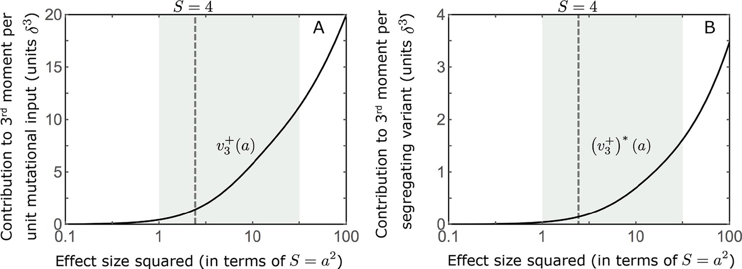
The distribution of the 3^rd central moment at equilibrium.

We show the positive/negative contribution to the 3^rd central moment per unit mutational input (A) (based on Equation A3-34) and per segregating variant (B), as a function of effect size squared. The contributions become substantial for large effect sizes, i.e., when $S = a^{2} ≫ 4$ .

Appendix 3—figure 8

Download asset Open asset

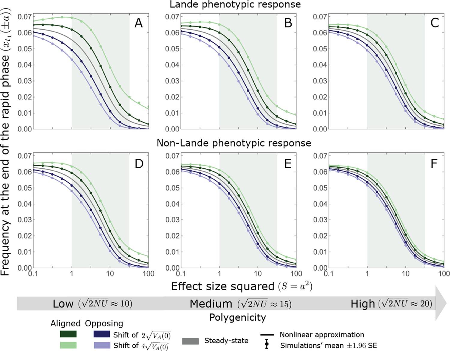
The nonlinear approximation accurately predicts average allele frequencies at the end of the rapid phase for a wide range of model parameters.

The simulation results were generated using the *single allele* simulation, as described in Section 2.1; errors are not visible because they are smaller than the points. The analytic predictions were based on the nonlinear approximations (Equations A3-40 and A3-48) averaged over the initial MAF distribution (Equation A3-27) with the corresponding parameters. As expected, when polygenicity is lower and shifts are larger the expected changes to allele frequencies are greater (compare A with C and D with F). Perhaps less obvious, despite the fact that our nonlinear approximation relies on Lande’s approximation, it performs well even in the cases with non-Lande phenotypic dynamics (**D–F**).

Appendix 3—figure 9

Download asset Open asset

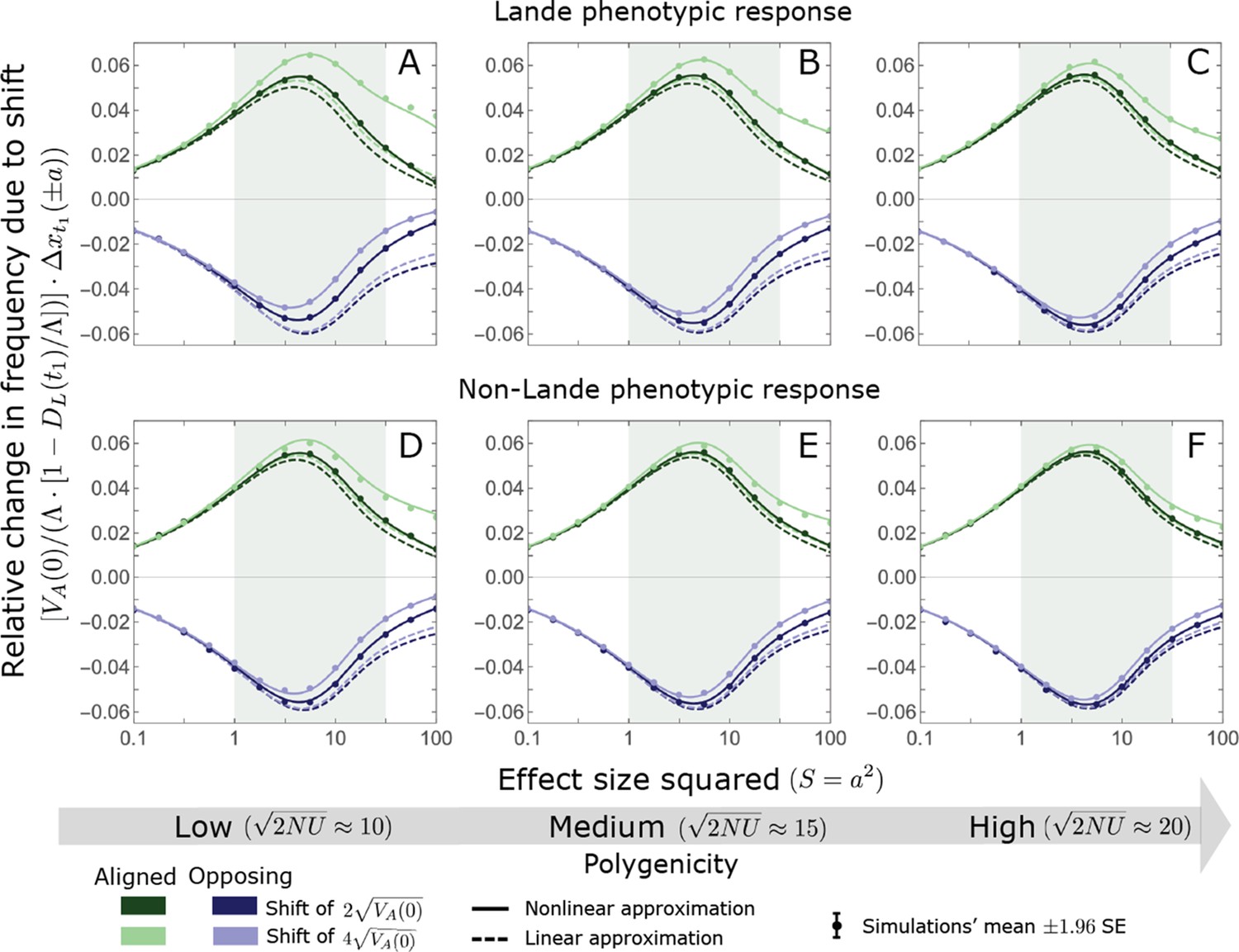
A comparison of the linear and nonlinear approximations with simulation results.

The simulation results were generated using the *single allele* simulation, as described in Section 2.1; errors are not visible because they are smaller than the points. The analytic predictions were based on the linear (Equations A3-40 and A3-45) and nonlinear (Equations A3-40 and A3-48) approximations averaged over the initial MAF distribution (Equation A3-27) with the corresponding parameters. The nonlinear approximation is quite accurate throughout and substantially more accurate than the linear approximation for larger effect sizes and low polygenicity (see, e.g., A, B, and D). In the linear approximation, frequency changes with directional selection alone scale with $Λ / V_{A} (0) \cdot (1 - D_{L} (t_{1}) / Λ)$ (Equations A3-39, A3-40 and A3-45). We therefore normalized the frequency changes by this factor to make the results for the two shift sizes and three extents of polygenicity comparable.

Appendix 3—figure 10

Download asset Open asset

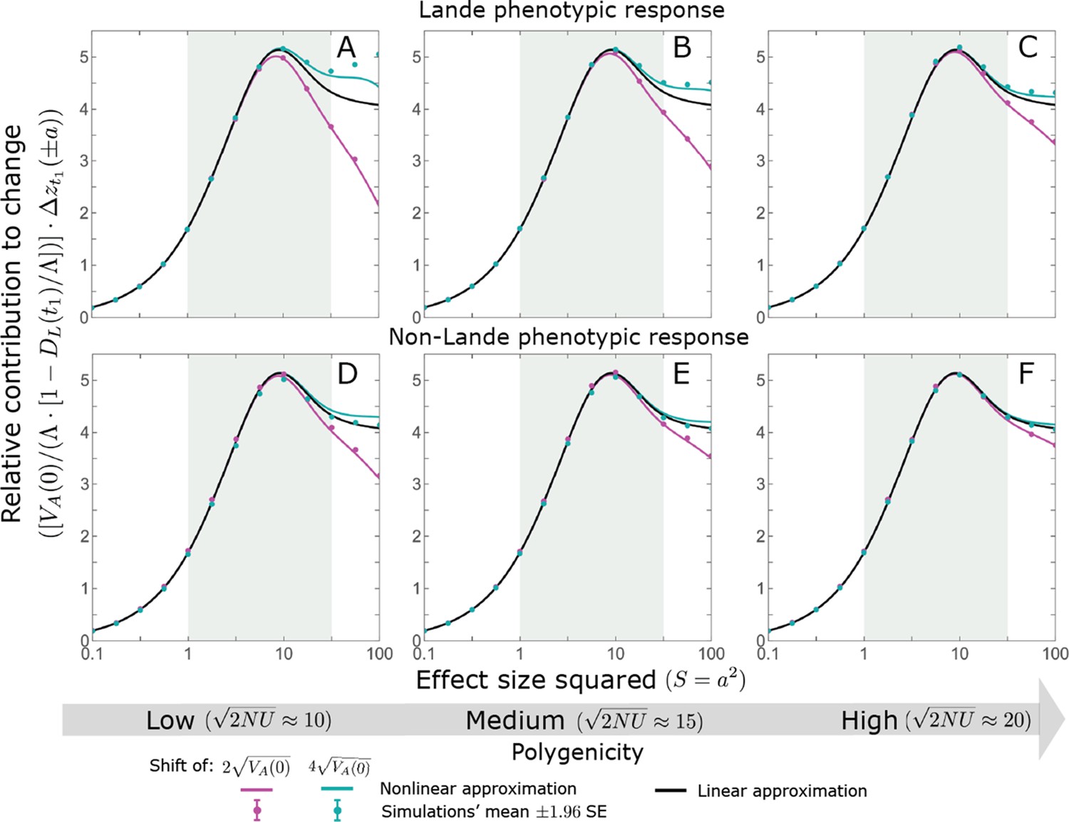
The allelic contribution to change in mean phenotype during the rapid phase.

The simulation results were generated using the *single allele* simulation, as described in Section 2.1; errors are not visible because they are smaller than the points. The analytic predictions were based on the linear (Equations A3-53 and A3-54 or Equation 13 in the main text) and nonlinear (Equations A3-48, A3-53 and A3-50) approximations with the corresponding parameters. As for the frequency changes, the nonlinear approximation for the expected contribution to change is quite accurate throughout and substantially more accurate than the linear approximation for larger effect sizes and low polygenicity (see, e.g. A and B). In the linear approximation, the contribution to change in mean phenotype scales with $Λ / V_{A} (0) \cdot (1 - D_{L} (t_{1}) / Λ)$ (see Equations A3-53 and A3-54). We therefore normalized the contributions by this factor to make them comparable for different initial variances and shift sizes.

Appendix 3—figure 11

Download asset Open asset

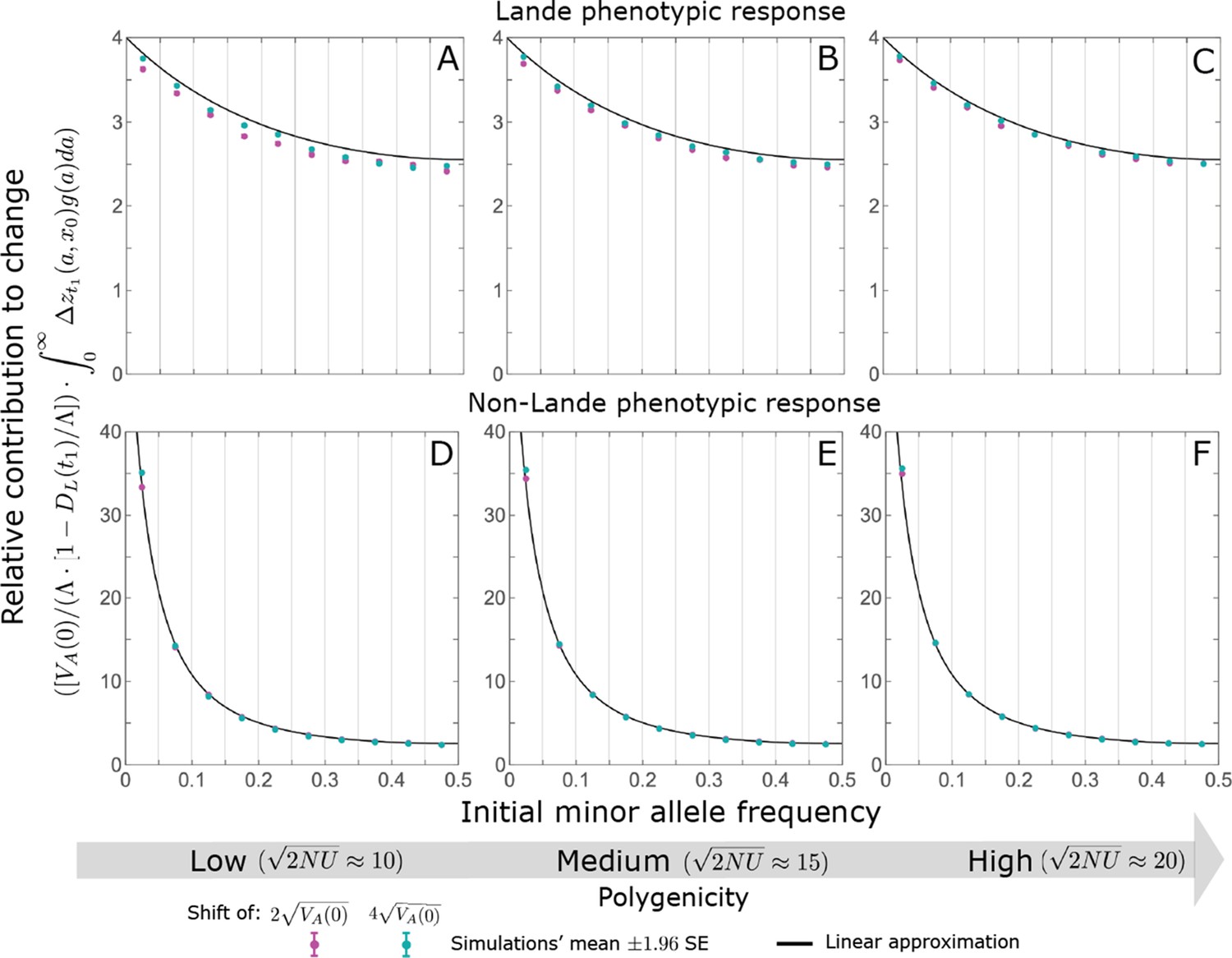
The relative contribution to change in mean phenotype during the rapid phase coming from different initial MAFs is well approximated by the relative contribution to phenotypic variance at equilibrium, as predicted by the linear approximation (Equations A3-52 and A3-54 or Equation 12 in the main text).

The simulation results were generated using the *all alleles* simulation, as described in Section 2.1. These results were binned by initial minor allele frequency (with boundaries between the bins marked by the light grey vertical lines) and the total contributions of alleles in frequency bin $(x_{1}, x_{2})$ is divided by the total mutational input per generation times the size of the bin, $2 N U (x_{2} - x_{1})$ . As in Appendix 3—figure 10, we normalized the contributions by $Λ / V_{A} (0) \cdot (1 - D_{L} (t_{1}) / Λ)$ to make them comparable for different initial variances and shift sizes. Errors are often not visible because they are smaller than the points.

Appendix 3—figure 12

Download asset Open asset

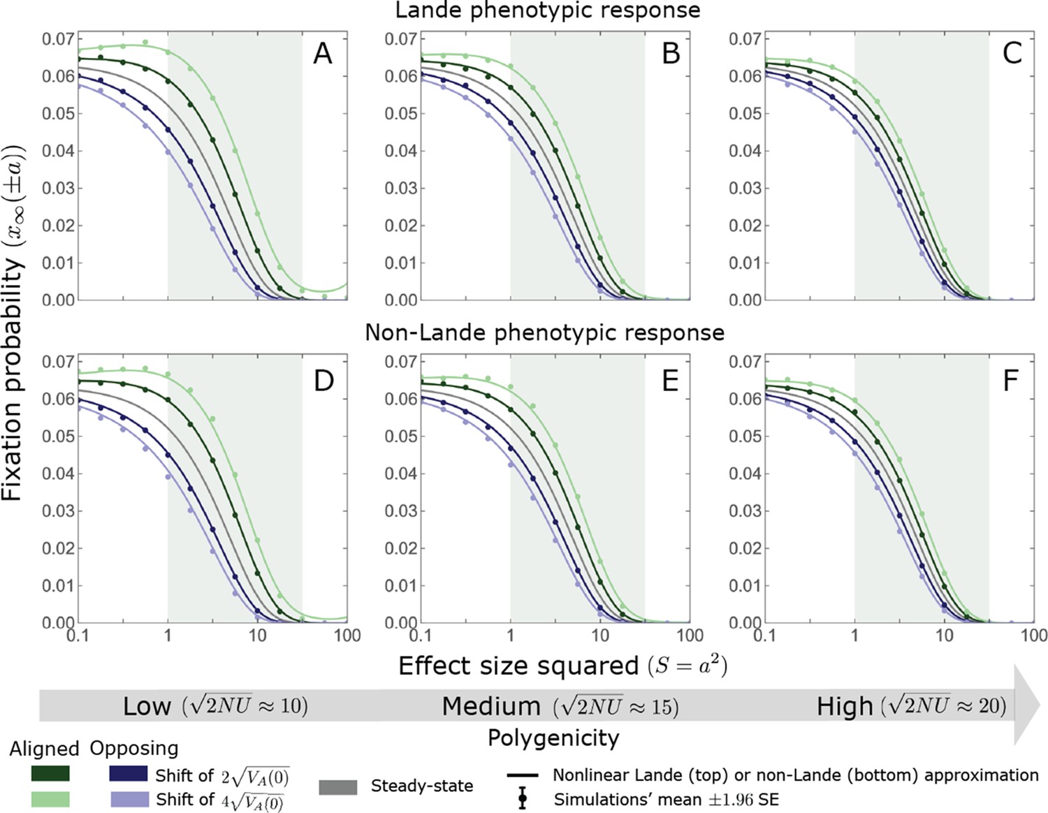
For small and intermediate alleles, changes in fixation probability are fairly small relative to the fixation probability at equilibrium.

The simulation results were generated using the *single allele* simulation, as described in Section 2.1; errors are not visible because they are smaller than the points. The analytic predictions were based on the nonlinear Lande (Equations A3-60, A3-84 and A3-85) and non-Lande (Equations A3-60, A3-88 and A3-89) approximations, averaged over the initial MAF distribution (Equation A3-27) with the corresponding parameters.

Appendix 3—figure 13

Download asset Open asset

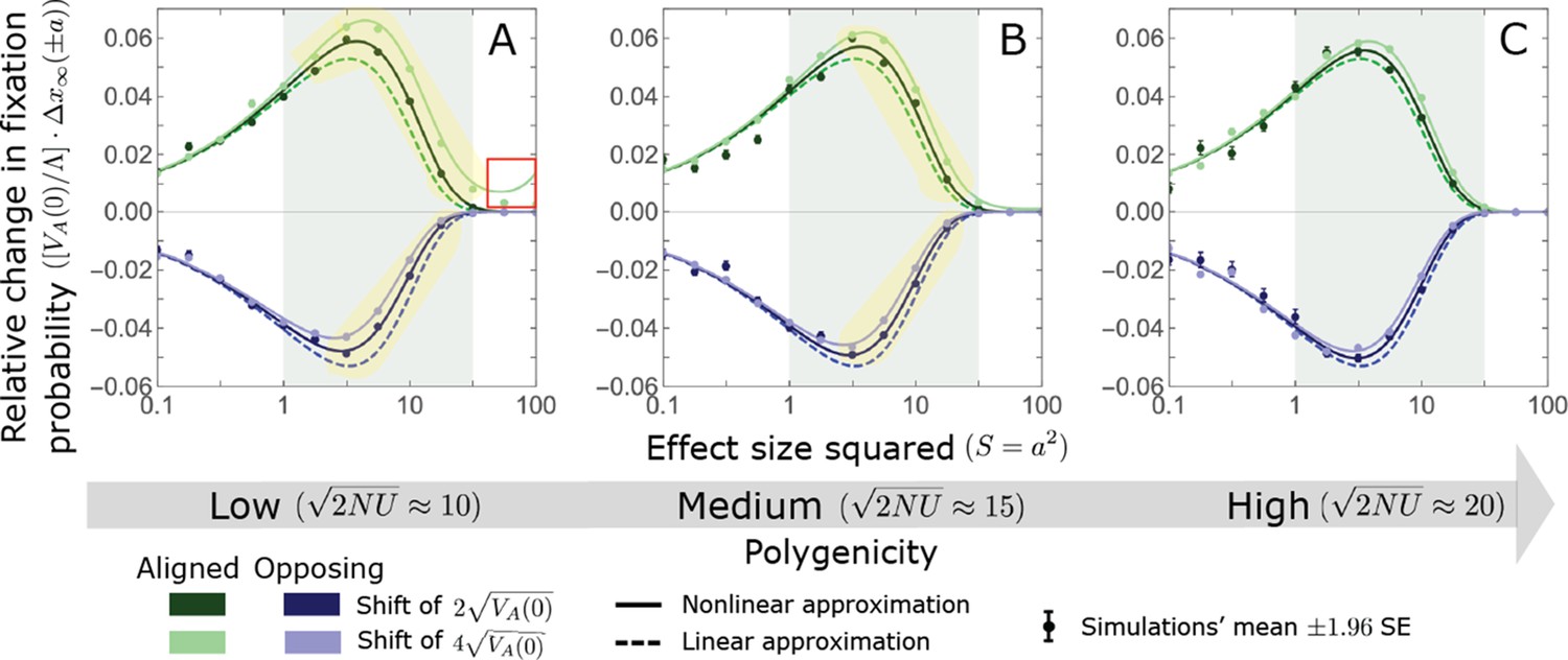
The Lande case: A comparison the linear and nonlinear approximations for the expected change in fixation probability of alleles already present at the time of the shift.

The simulation results were generated using the *single allele* simulation, as described in Section 2.1; errors are often not visible because they are smaller than the points. The analytic predictions were based on the linear Lande (Equations A3-60 and A3-61) and nonlinear Lande (Equations A3-60, A3-84 and A3-85) approximations averaged over the initial MAF distribution (Equation A3-27) with the corresponding parameters. The nonlinear Lande approximation performs better than the linear Lande approximation for alleles with large and intermediate effects, especially when polygenicity is lower (see the golden shaded regions in A and B). In the linear approximation, the change in fixation probability scales with $Λ / V_{A} (0)$ (Equation A3-61). We therefore divided the changes in fixation probability by this factor to make them comparable for different initial variances and shift sizes. Note that with this normalization, the linear curves for the two shifts are identical, which is why only one is visible.

Appendix 3—figure 14

Download asset Open asset

The Lande case: the long-term relative contribution to the change in mean phenotype coming from different initial MAFs is approximately constant.

The simulation results were generated using the *all alleles* simulation, as described in *Choice of simulation parameters*. The results for a given case were binned by initial minor allele frequency (with boundaries between the bins marked by the light grey vertical lines). The total contributions of alleles in frequency bin $(x_{1}, x_{2}]$ is divided by the total mutational input per generation times the size of the bin, $2 N U (x_{2} - x_{1})$ . The analytic predictions were based on the linear Lande approximation (Equation A3-63 or Equation 19 in the main text).

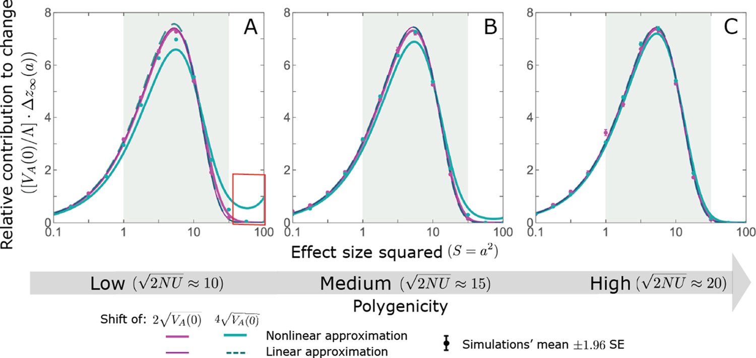
Appendix 3—figure 15

Download asset Open asset

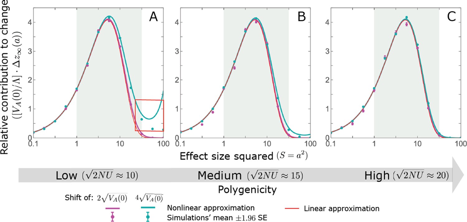
The Lande case: As predicted by the linear approximation, the long-term relative contribution to the change in mean phenotype coming from standing variation scales with $Λ / V_{A} (0)$ .

Both the linear and nonlinear Lande approximation are fairly accurate for alleles with small effects. When polygenicity is low, the nonlinear Lande approximation is more accurate for alleles with intermediate effects (see the teal line in A and B). Both approximations perform badly for large effect alleles when the polygenicity is low and the shift is large (the red box in A). However, in the Lande case, we expect very few alleles to have large effect sizes. The simulation results were generated using the *single allele* simulation, as described in Section 2.1; errors are often not visible because they are smaller than the points. The analytic predictions were based on the linear Lande (Equation A3-64 or Equation 20 in the main text) and nonlinear Lande (Equations A3-84–A3-A88) approximations.

Appendix 3—figure 16

Download asset Open asset

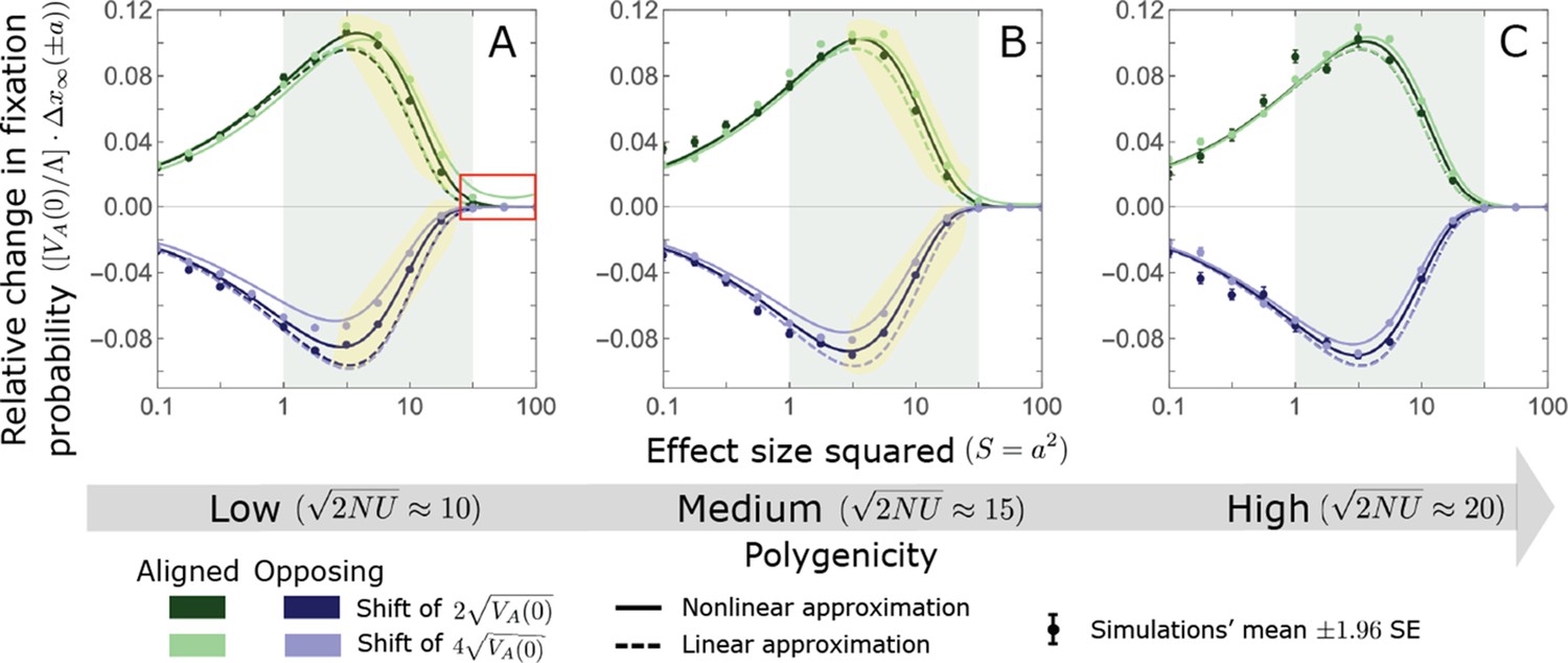
The non-Lande case: A comparison of the linear and nonlinear approximations for the expected change in fixation probability of alleles segregating at the time of the shift.

The simulation results were generated using the *single* allele simulation, as described in Section 2.1; errors are often not visible because they are smaller than the points. The analytic predictions were based on the linear non-Lande (Equations A3-60 and A3-70) and nonlinear non-Lande (Equations A3-60, A3-88 and A3-89) approximations averaged over the initial MAF distribution (Equation A3-27) with the corresponding parameters. The nonlinear approximation performs better than the linear one for intermediate effect alleles when polygenicity is low (see the gold shaded regions in A and B). As in Appendix 3—figure 13, we normalize the changes in fixation probability by $Λ / V_{A} (0)$ to make them comparable for different initial variances and shift sizes (Equation A3-61).

Appendix 3—figure 17

Download asset Open asset

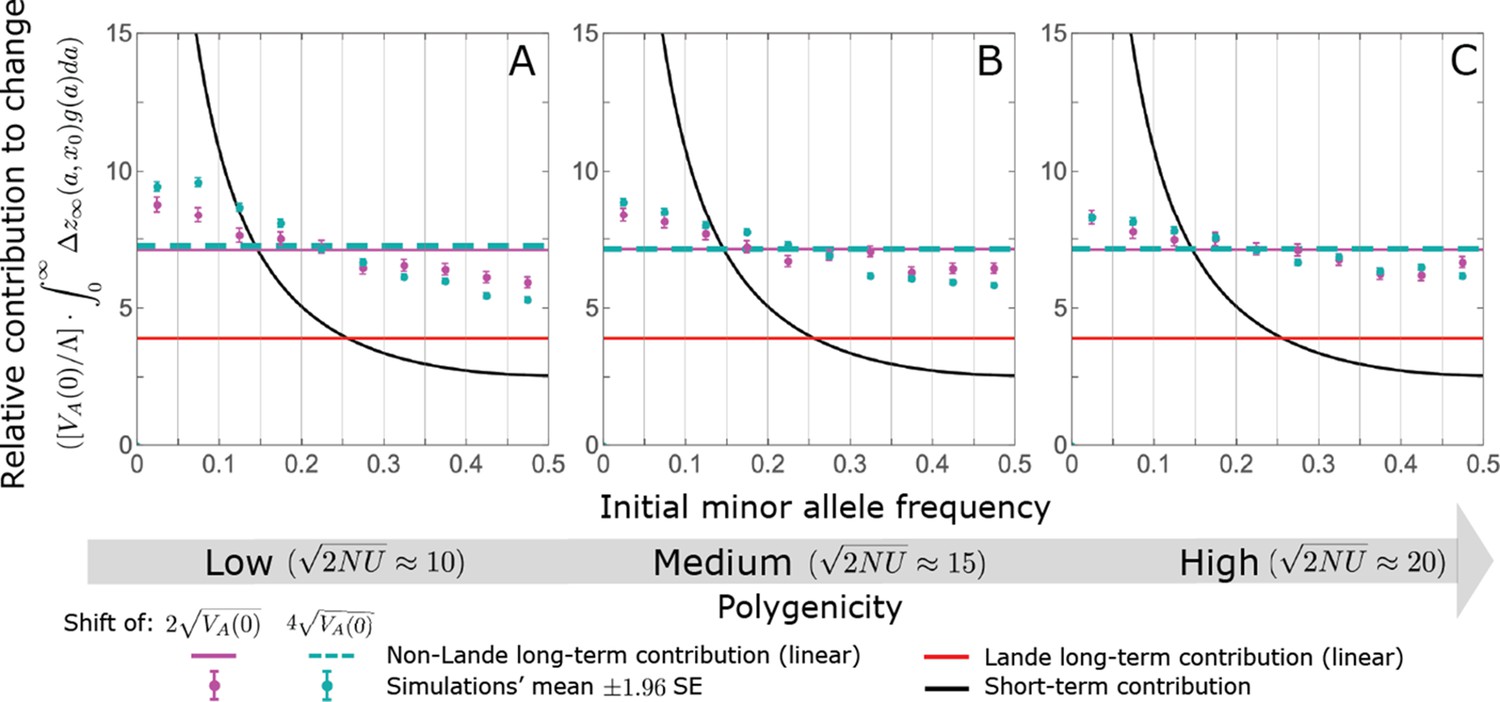
The non-Lande case: The long-term relative contribution to the change in mean phenotype coming from different initial MAFs is approximately constant, with low initial MAF alleles contributing slightly more than high initial MAF alleles.

The slight excess in the contribution of alleles with low initial MAF is especially pronounced when the shift is large and the polygenicity is low. The simulation results were generated using the *all alleles* simulation, as described in Section 2.1. We calculate the relative contribution of alleles in each MAF bin $(x_{1}, x_{2})$ (between the gray gridlines) by dividing the contribution of fixations in the bin by the total mutational input per generation times the size of the bin, $2 N U (x_{2} - x_{1})$ . The analytic predictions were based on the linear non-Lande approximation (Equation A3-71 or Equation 24 in the main text).

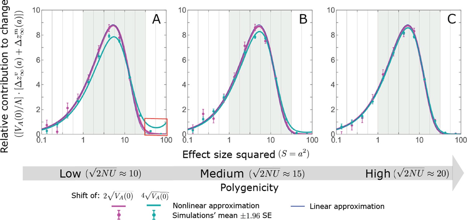
Appendix 3—figure 18

Download asset Open asset

The non-Lande case: As predicted by the linear approximation, the long-term relative contribution to the change in mean phenotype coming from standing variation scales with $Λ / V_{A} (0)$ .

Both the linear and nonlinear approximations predict the long-term relative contribution to the change in mean phenotype fairly well. However, when polygenicity is low and the shift is large, the nonlinear approximation overestimates the proportion of the change in mean due to large effect alleles (see the red box in A). The simulation results were generated using the *single allele* simulation, as described in Section 2.1; errors are often not visible because they are smaller than the points. The analytic predictions were based on the linear non-Lande (Equation A3-72 or Equation 25 in the main text) and nonlinear non-Lande (Equations A3-86–A3-89) approximations.

Appendix 3—figure 19

Download asset Open asset

The non-Lande case: As predicted by the linear approximation, the long-term contribution, per unit mutational input, to the change in mean phenotype coming from standing variation and new mutations scales with $(1 + C) \cdot Λ / V_{A} (0)$ (Equation A3-83).

Both the linear and nonlinear approximations perform fairly well. However, when the polygenicity is low and the shift is large, the nonlinear approximation overestimates the proportion of the change in mean due to large effect standing variation (Appendix 3—figure 18) and therefore overestimates the proportion contribution coming from *all* large effect alleles (see the red box in A). The simulation results were generated using the *all allele* simulation, as described in Section 2.1. We calculate the relative contribution of alleles in each effect size squared bin $(a_{1}^{2}, a_{2}^{2}]$ (between the gray gridlines) by dividing the contribution of fixations in the bin by the total mutational input per generation times the size of the bin, $2 N U \int_{a_{1}}^{a_{2}} g (a) d a$ . The analytic predictions were based on the linear non-Lande (Equation A3-83 or Equation 28 in the main text) and nonlinear non-Lande (Section 5.4.3) approximations with the corresponding parameters.

Appendix 3—figure 20

Download asset Open asset

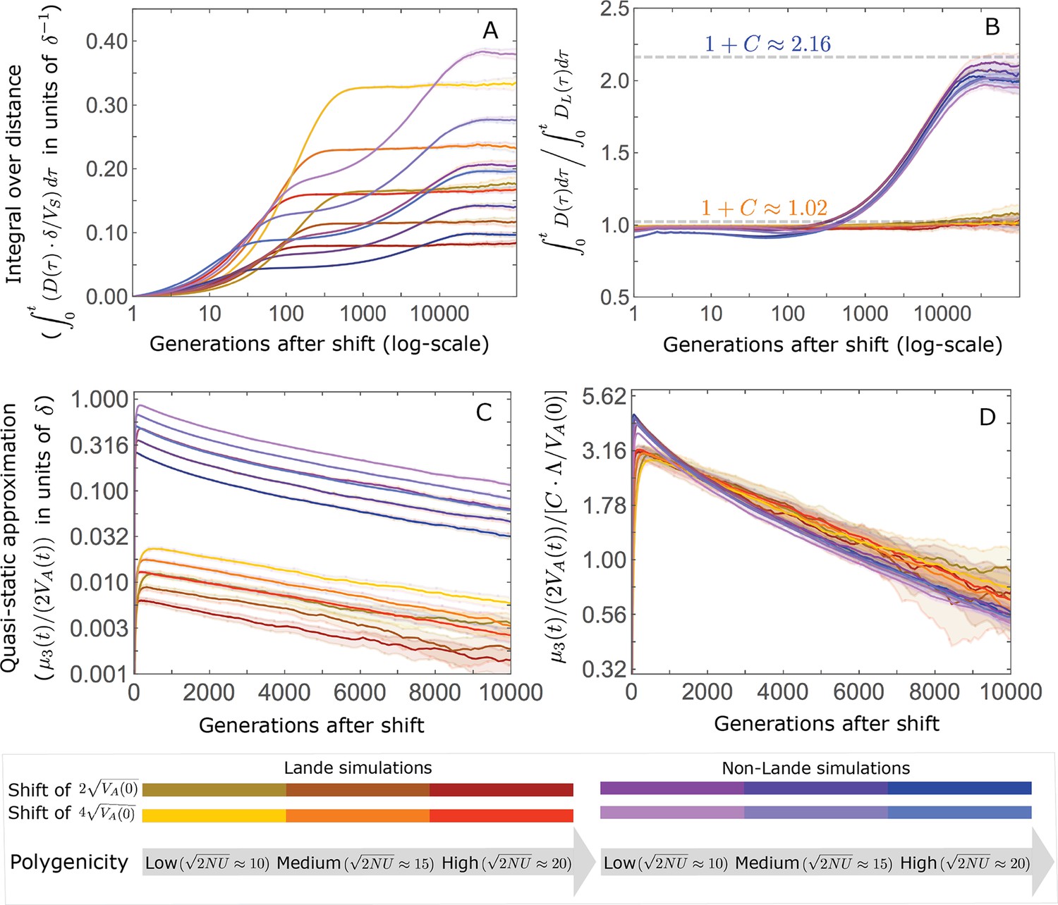
The trajectory of the mean integral over the phenotypic distance from the optimum is largely determined by Lande’s approximation and by the amplification $C$ .

(A) The integral distance from the optimum as a function of time after the shift. In Lande cases, the integral nears the asymptote $\int_{0}^{\infty} (D_{L} (τ) \cdot δ / V_{S}) d τ = (Λ \cdot δ) / V_{A} (0)$ at the end of the rapid phase, whereas in non-Lande cases, the integral continues to increase substantially during equilibration. (B) The integral over the distance scaled by the integral over the distance obtained from Lande’s approximation as a function of time. The phenotypic trajectories corresponding to the Lande and to the non-Lande cases with different parameter values stack up, illustrating that, to a good approximation, the impact of polygenicity and shift size are captured by Lande’s approximation; the long-term impact of the effect size distribution, manifest in the non-Lande cases, is largely captured by $C$ . (C) The quasi-static approximation of the distance as a function of time is affected by all of the parameters. (D) The quasi-static approximation of the distance scaled by $C \cdot (Λ \cdot δ) / V_{A} (0)$ as a function of time. During the equilibration phase, the phenotypic trajectories corresponding to different parameter values stack up, illustrating that, to a good approximation, the effects of all of the parameters is captured by this compound parameter. The simulation results were generated using the *all allele* simulation, as described in Section 2.1.

Appendix 3—figure 21

Download asset Open asset

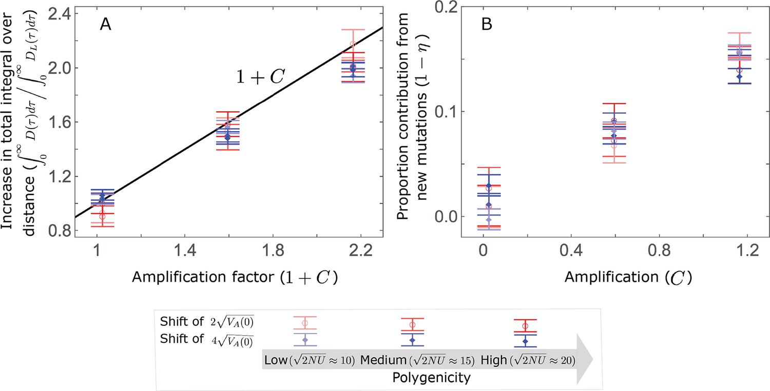
The amplification $C$ largely determines the increase in the total integral over distance, where $\int_{0}^{\infty} D (τ) d τ / \int_{0}^{\infty} D_{L} (τ) / V_{S} d τ \approx 1 + C$ (A); moreover, the proportion of long-term phenotypic change arising from new mutations ( $1 - η$ ), is approximately proportional to $C$ (B).

As an illustration, we show the averages of these quantities over 500 *all alleles* simulations assuming $N = 10^{4}$ , with the three extents of polygenicity and two shift sizes specified in the legend, and with three distributions of effect sizes: our two standard cases with an exponential distribution of effect sizes squared, with $E (a^{2}) = 1$ and $C \approx 0.02$ (our Lande case) and with $E (a^{2}) = 16$ and $C \approx 1.16$ (our non-Lande case), and an additional intermediate case with $a^{2} \sim Gamma [2 / 9, 27]$ and $C \approx 1.16$ .

Appendix 3—figure 22

Download asset Open asset

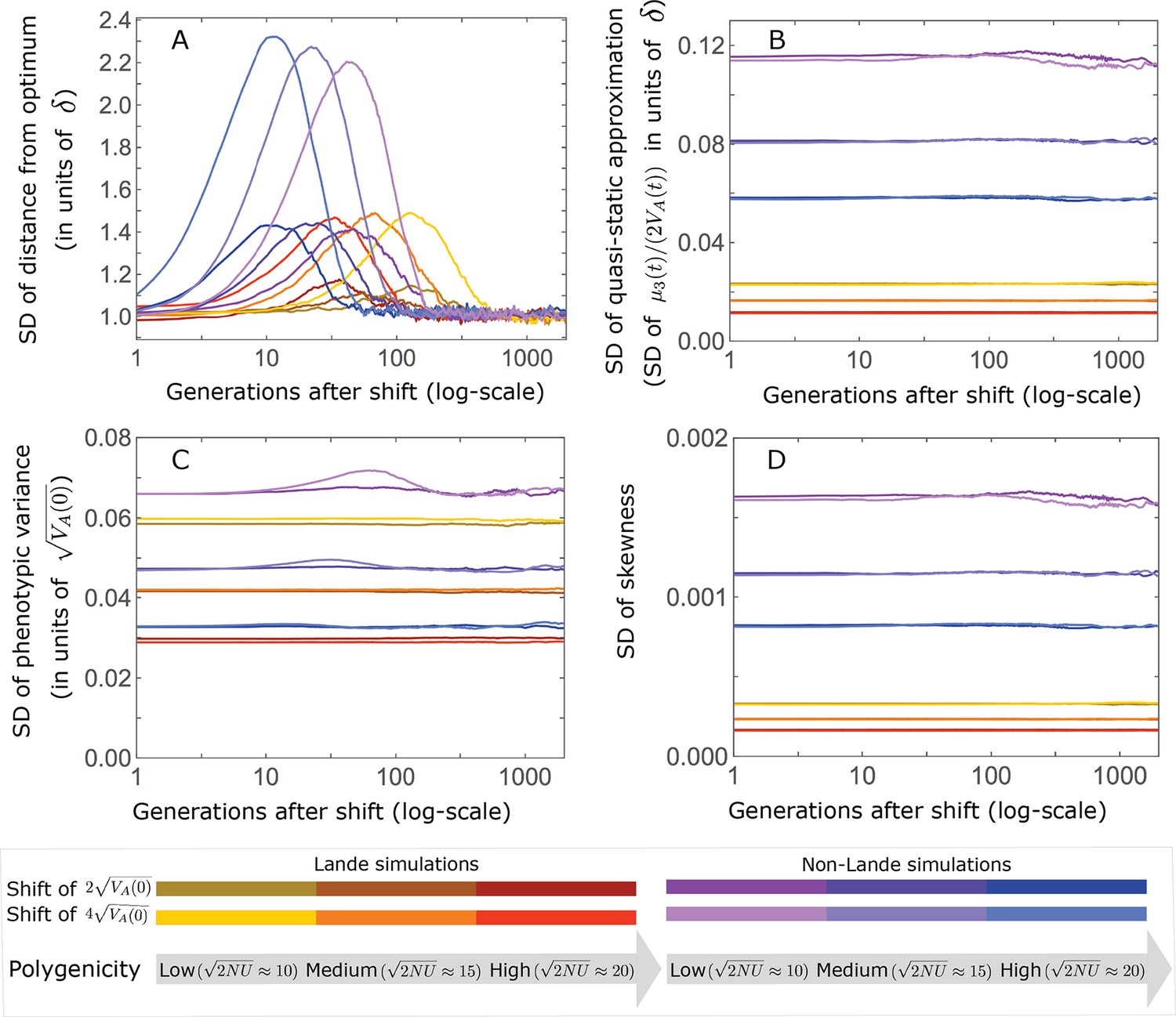
Variation in summaries of the phenotypic distribution as a function of time after the shift in optimum.

(A) The standard deviation of the population’s mean distance from the optimum. (B) The standard deviation of the quasi-static approximation for the population’s mean phenotypic distance from the optimum, that is, the SD of $μ_{3} (t) / (2 V_{A} (t))$ (Equation 6 in the main text). (C) The standard deviation of the phenotypic variance measured relative to the expected variance at equilibrium (Equation A3-30). (D) The standard deviation of the skewness of the phenotypic distribution (i.e., $μ_{3} (t) / V_{A}^{3 / 2} (t)$ ). The simulation results were generated using the *all allele* simulation, as described in Section 2.1.

Appendix 3—figure 23

Download asset Open asset

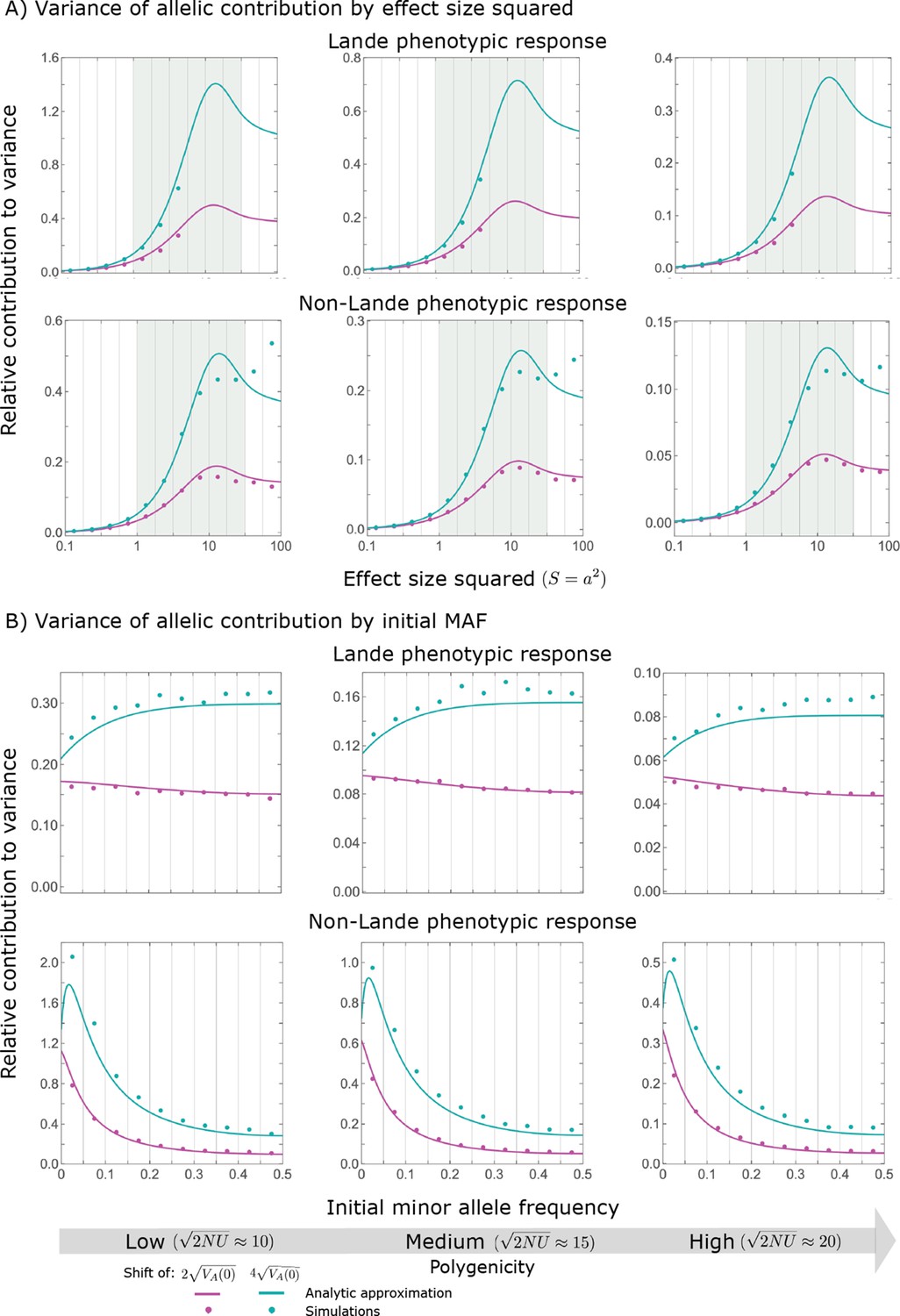
Variance of the allelic contribution to phenotypic adaptation in the rapid phase, as a function of effect size squared (A) and initial MAF (B).

The results of our *all allele* simulation are compared to our corresponding analytic approximations (see text), with the parameters for each case detailed in Section 2.1. Simulation results are shown for bins (demarked by the gray vertical lines), where in (A) we divided the variance of the allelic contribution in bin $(a_{1}^{2}, a_{2}^{2}]$ by the corresponding expected mutational input $2 N U \cdot \int_{a_{1}}^{a_{2}} g (a) d a$ , and in (B) we divided the variance in bin $(x_{1}, x_{2}]$ by $2 N U \cdot (x_{2} - x_{1})$ . In the Lande case, we only show the results for $a^{2} < 10$ , because fewer than $0.005 %$ of new mutations fall above that range.

Appendix 3—figure 24

Download asset Open asset

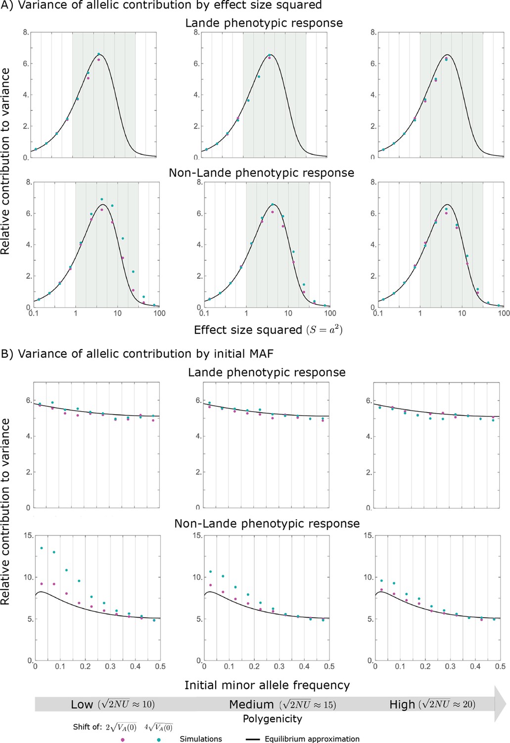
Variance of the allelic contribution to phenotypic adaptation in the equilibration phase, as a function of effect size squared (A) and initial MAF (B).

The results of our *all allele* simulation are compared to our corresponding analytic approximations (see text), with the parameters for each case detailed in Section 2.1. Simulation results are shown for bins (demarked by the gray vertical lines), where in (A) we divided the variance of the allelic contribution in bin $(a_{1}^{2}, a_{2}^{2}]$ by the corresponding expected mutational input $2 N U \cdot \int_{a_{1}}^{a_{2}} g (a) d a$ , and in (B) we divided the variance in bin $(x_{1}, x_{2}]$ by $2 N U \cdot (x_{2} - x_{1})$ . In the Lande case, we only show the results for $a^{2} < 10$ , because fewer than $0.005 %$ of new mutations fall above that range.

Appendix 3—figure 25

Download asset Open asset

Our definition of the end of the rapid phase, $t_{1}$ , roughly captures the change in phenotypic dynamic in the non-Lande case.

At least in these non-Lande cases, $D_{L} (t_{1})$ is quite close to $δ$ and the quasi-static approximation (Equation 6 in the main text) becomes accurate shortly after $t_{1}$ . The simulation results were generated using the *all allele* simulation, as described in Section 2.1.

Appendix 3—figure 26

Download asset Open asset

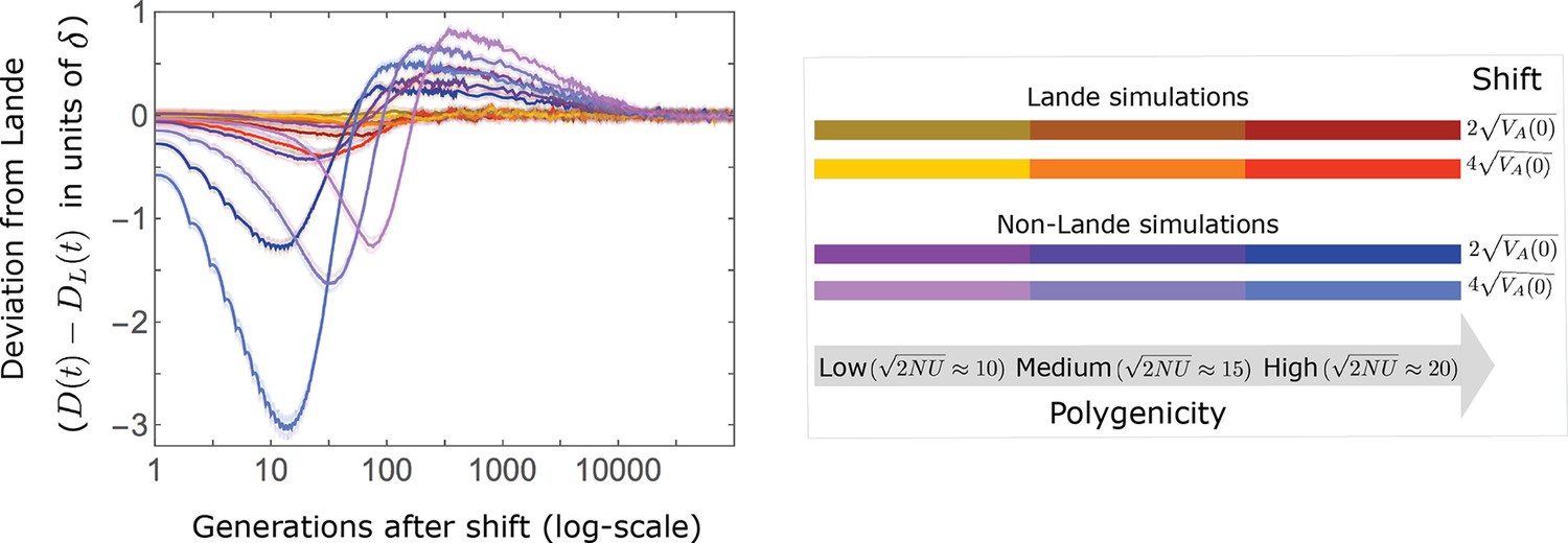
Deviations from Lande’s approximation as a function of time after the shift.

In the Lande case, i.e., when $C ≪ 1$ , the mean distance from the new optimum is well approximated by $D_{L} (t)$ . Deviations increase with shift size and extent of polygenicity (as seen, e.g., in the red curve), primarily due to a moderate increase in phenotypic variance during the rapid phase. The increase in the 3^rd phenotypic moment is minimal, which is why, in this case, there are no substantial long-term deviations. In the non-Lande case, the distance from the optimum decays faster than predicted by Lande’s approximation ( $D (t) - D_{L} (t) < 0$ ) during the rapid phase, because of the increase in phenotypic variance. The increase in the 3^rd central moment during the rapid phase leads to a slower decay than predicted by Lande’s approximation during the equilibration phase. Even in the non-Lande case, however, we always find the distance from the optimum during equilibration to be smaller than $δ$ . The simulation results were generated using the *all allele* simulation, as described in Section 2.1.

Appendix 3—figure 27

Download asset Open asset

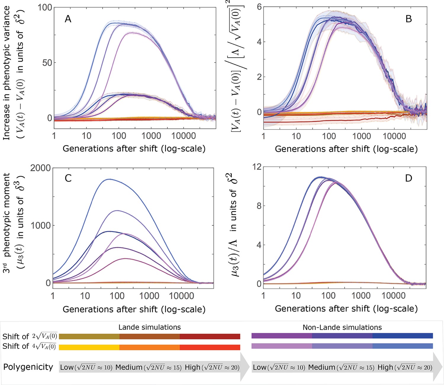
The increase in the 2^nd and 3^rd central moments of the phenotypic distribution.

(A and C) The increase is largely driven by alleles with large effects. Specifically, there are substantial increases only in the non-Lande cases, that is, those with an abundance of new mutations with $a^{2} > 4$ . (B and D) We conjecture that the compound parameters that largely determine the increase in moments are: ${(Λ / \sqrt{V_{A} (0)})}^{2}$ for the 2^nd central moment (B) and $Λ / δ$ for the 3^rd. Note that the slight differences among curves in the non-Lande case are short-lived (time is measured on a log-scale). The simulation results were generated using the *all allele* simulation, as described in Section 2.1.

Appendix 3—figure 28

Download asset Open asset

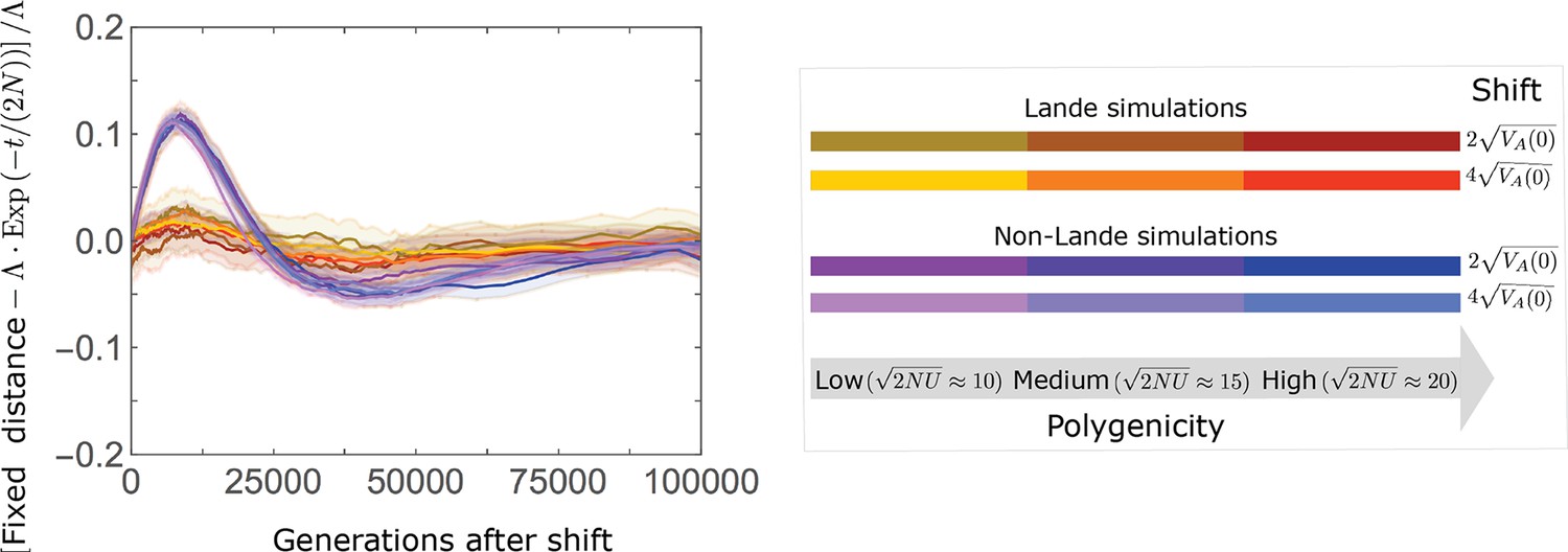
The approach of the fixed background to the new optimum is well approximated by $Λ e^{- t / (2 N)}$ , with deviations proportional to the shift size multiplied by a function that depends largely on $C$ .

We speculate that the (positive) deviations on the intermediate time-scale (e.g., around generation $1000$ ) in the non-Lande case are primarily due to the slower accumulation of fixations from new mutations, which contribute substantially in this case, whereas the (negative) deviations on the slightly longer time-scale (e.g. around generation $4000$ ) are due to the cumulative effect of prolonged weak directional selection, which has a substantial effect in this case. The simulation results were generated using the *all allele* simulation, as described in Section 2.1.

Tables

Appendix 1—table 1

Summary of notation.

Symbol	Definition
$N$	Population size
$U$	Expected number of mutations per gamete per generation affecting the trait
$V_{S}$	Width of the Gaussian fitness function ( $- 1 / V_{S}$ is the quadratic selection gradient)
$δ$	Typical magnitude of fluctuations around the optimum at equilibrium ( $= \sqrt{V_{S} / (2 N)}$ )
$a$	The magnitude of an allele’s effect on the trait
$S$	An allele’s scaled selection coefficient at equilibrium ( $= a^{2}$ in units of $δ^{2}$ )
$g (a)$	The mutational distribution of phenotypic magnitudes
$Λ$	The size of the shift in optimum
$t$	Time after shift in optimum
$V_{A} (t)$	The additive genetic variance at time $t$
$μ_{3} (t)$	The 3^rd central moment of the trait distribution at time $t$
$D (t)$	Distance of the mean phenotype from the optimum at time $t$
$D_{L} (t)$	Lande’s approximation for $D (t)$
$t_{1}$	The time of the end of the rapid phase
$x_{t} (a, x_{0})$	Expected frequency of an allele with effect $a$ and initial MAF $x_{0}$ , at time $t$
$Δ x_{t}^{*} (a, x_{0})$	Expected frequency difference between opposite alleles at time $t$ (≡ $x_{t} (a, x_{0}) - x_{t} (- a, x_{0})$ )
$Δ z_{t}^{*} (a, x_{0})$	Expected contribution to phenotypic change of a pair of opposite alleles at time $t$
$v^{*} (a, x)$	An allele’s contribution to phenotypic variance ( $= 2 a^{2} x (1 - x)$ )
$Δ x_{d}^{*} (a, x_{0})$	Expected frequency difference between opposite alleles due to an instantaneous pulse of directional selection (≡ $x_{d} (a, x_{0}) - x_{d} (- a, x_{0})$ )
$Δ z_{d}^{*} (a, x_{0})$	Expected contribution to phenotypic change of a pair of opposite alleles after an instantaneous pulse of directional selection
$Δ z_{t} (a, x_{0}),$ $Δ z_{t} (a)$	Expected contribution to phenotypic change per unit mutational input of opposite alleles with magnitude $a$ , or with magnitude $a$ and initial MAF $x_{0}$ , at time $t$
$v (a, x_{0}),$ $v (a)$	Equilibrium density of phenotypic variance per unit mutational input of alleles with magnitude $a$ , or with magnitude $a$ and initial MAF $x_{0}$
$π (a, x)$	Fixation probability of an allele with magnitude $a$ and initial frequency $x$ under stationary stabilizing selection and genetic drift
$f (a)$	Relative long-term contribution to phenotypic change
$A$	Amplification of the long-term contribution to phenotypic change from standing variation
$C$	Amplification of the long-term contribution to phenotypic change $= \int v (a) g (a) d a / \int f (a) g (a) d a - 1$

Appendix 1—table 2

Summary of assumptions on parameters.

Assumption	Interpretation
$\sqrt{2 N U} ≫ 1$	The trait is highly polygenic
$U = L u \leq 0.02$	The mutation rate per gamete is sufficiently low such that $V_{A} (0) ≪ V_{S}$
$a / \sqrt{V_{S}} ≪ 1$	Directional selection coefficients of alleles satisfy $s_{d} ≪ 1$
$g (a)$ with a substantial portion satisfying $a^{2} ⪆ 1$	A substantial proportion of incoming mutations are not effectively neutral
$g (a) = g (- a)$	Mutational input is symmetric
$Λ > δ$	The shift is not negligible (i.e. larger than the typical equilibrium fluctuations in mean phenotype)
$Λ ⪅ \sqrt{V_{S}}$	Maximal directional selection coefficients satisfy $s_{d} ≪ 1$
$Λ / \sqrt{V_{A} (0)} ⪅ 1 / 2 \cdot \sqrt{2 N U}$	Moving the trait mean to the new optimum requires only small average frequency changes per segregating site

Additional files

Transparent reporting form: https://cdn.elifesciences.org/articles/66697/elife-66697-transrepform1-v3.docx
Download elife-66697-transrepform1-v3.docx

Download links

A two-part list of links to download the article, or parts of the article, in various formats.

Downloads (link to download the article as PDF)

Article PDF

Open citations (links to open the citations from this article in various online reference manager services)

Mendeley

Cite this article (links to download the citations from this article in formats compatible with various reference manager tools)

Laura Katharine Hayward
Guy Sella

(2022)

Polygenic adaptation after a sudden change in environment

eLife 11:e66697.

https://doi.org/10.7554/eLife.66697

Share this article

Cite this article

The evolutionary scenario.

The phenotypic response to a shift in optimal phenotype.

A cartoon of allele dynamics.

The allelic response during the rapid phase.

The long-term (fixed) allelic contribution to phenotypic adaptation.

The genetic basis of adaptation turns over during the equilibration phase.

While long-term phenotypic adaptation arises from an excess in fixations of aligned relative to opposing alleles, this excess and its effect on the total number of fixations is typically small.

Equilibrium around the new optimum is restored on a time scale of 2 ⁢ N generations after the shift.

While directional selection during the rapid phase increases the frequency of aligned alleles relative to opposing ones, the frequency of aligned alleles does not necessarily increase.

Stabilizing selection during the equilibration phase causes turnover in the genetic basis of adaptation.

The long-term phenotypic contribution of minor alleles is amplified if they start above a critical initial frequency, which depends on their magnitude, and it is diminished if they start below this critical MAF.

Our simulation parameter values are chosen to span as wide a range as possible given our conditions on them.

Comparison of our main results about the phenotypic dynamics with corresponding results from the full model simulations.

Comparison of our main results about the allele dynamics with the corresponding results of the full model simulations.

Allelic densities at equilibrium.

The distribution of variance at equilibrium.

An upper bound on shift size measured in phenotypic standard deviations.

The distribution of the 3rd central moment at equilibrium.

The nonlinear approximation accurately predicts average allele frequencies at the end of the rapid phase for a wide range of model parameters.

A comparison of the linear and nonlinear approximations with simulation results.

The allelic contribution to change in mean phenotype during the rapid phase.

For small and intermediate alleles, changes in fixation probability are fairly small relative to the fixation probability at equilibrium.

The Lande case: A comparison the linear and nonlinear approximations for the expected change in fixation probability of alleles already present at the time of the shift.

The Lande case: the long-term relative contribution to the change in mean phenotype coming from different initial MAFs is approximately constant.

The Lande case: As predicted by the linear approximation, the long-term relative contribution to the change in mean phenotype coming from standing variation scales with Λ / V A ⁢ ( 0 ) .

The non-Lande case: A comparison of the linear and nonlinear approximations for the expected change in fixation probability of alleles segregating at the time of the shift.

The non-Lande case: The long-term relative contribution to the change in mean phenotype coming from different initial MAFs is approximately constant, with low initial MAF alleles contributing slightly more than high initial MAF alleles.

The non-Lande case: As predicted by the linear approximation, the long-term relative contribution to the change in mean phenotype coming from standing variation scales with Λ / V A ⁢ ( 0 ) .

The non-Lande case: As predicted by the linear approximation, the long-term contribution, per unit mutational input, to the change in mean phenotype coming from standing variation and new mutations scales with ( 1 + C ) ⋅ Λ / V A ⁢ ( 0 ) (Equation A3-83).

The trajectory of the mean integral over the phenotypic distance from the optimum is largely determined by Lande’s approximation and by the amplification C .

Variation in summaries of the phenotypic distribution as a function of time after the shift in optimum.

Variance of the allelic contribution to phenotypic adaptation in the rapid phase, as a function of effect size squared (A) and initial MAF (B).

Variance of the allelic contribution to phenotypic adaptation in the equilibration phase, as a function of effect size squared (A) and initial MAF (B).

Our definition of the end of the rapid phase, t 1 , roughly captures the change in phenotypic dynamic in the non-Lande case.

Deviations from Lande’s approximation as a function of time after the shift.

The increase in the 2nd and 3rd central moments of the phenotypic distribution.

The approach of the fixed background to the new optimum is well approximated by Λ ⁢ e - t / ( 2 ⁢ N ) , with deviations proportional to the shift size multiplied by a function that depends largely on C .

Summary of notation.

Summary of assumptions on parameters.

Transparent reporting form

Downloads (link to download the article as PDF)

Open citations (links to open the citations from this article in various online reference manager services)

Cite this article (links to download the citations from this article in formats compatible with various reference manager tools)

Equilibrium around the new optimum is restored on a time scale of $2 N$ generations after the shift.

The distribution of the 3^rd central moment at equilibrium.

The Lande case: As predicted by the linear approximation, the long-term relative contribution to the change in mean phenotype coming from standing variation scales with $Λ / V_{A} (0)$ .

The non-Lande case: As predicted by the linear approximation, the long-term relative contribution to the change in mean phenotype coming from standing variation scales with $Λ / V_{A} (0)$ .

The non-Lande case: As predicted by the linear approximation, the long-term contribution, per unit mutational input, to the change in mean phenotype coming from standing variation and new mutations scales with $(1 + C) \cdot Λ / V_{A} (0)$ (Equation A3-83).

The trajectory of the mean integral over the phenotypic distance from the optimum is largely determined by Lande’s approximation and by the amplification $C$ .

Our definition of the end of the rapid phase, $t_{1}$ , roughly captures the change in phenotypic dynamic in the non-Lande case.

The increase in the 2^nd and 3^rd central moments of the phenotypic distribution.

The approach of the fixed background to the new optimum is well approximated by $Λ e^{- t / (2 N)}$ , with deviations proportional to the shift size multiplied by a function that depends largely on $C$ .