Global constraints within the developmental program of the Drosophila wing
- Department of Engineering Sciences and Applied Mathematics, Northwestern University, United States
- NSF-Simons Center for Quantitative Biology, Northwestern University, United States
- Department of Molecular Biosciences, Northwestern University, United States
Figures
Figure 1 with 4 supplements
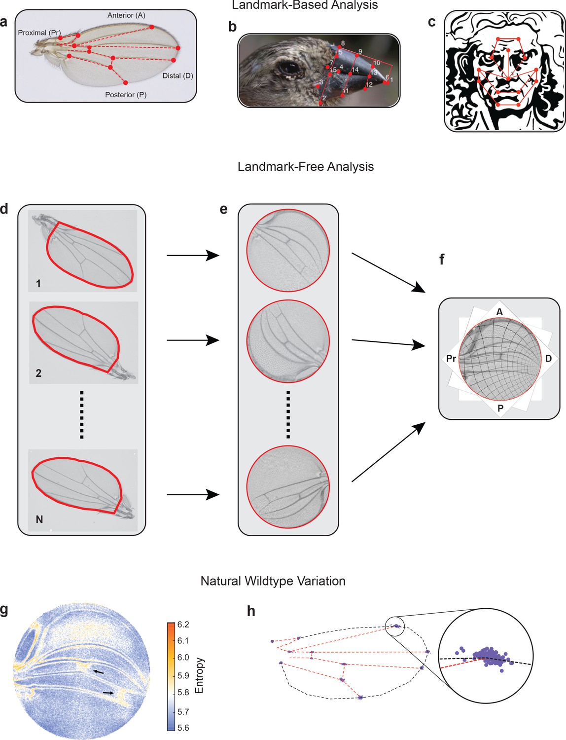
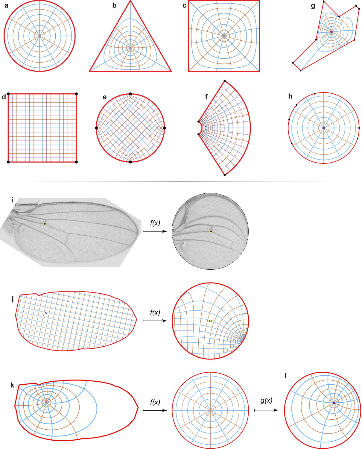
Landmark-free morphometrics.
(a–c) Standard landmarks (red) for Procrustes analysis of a Drosophila wing (a), the beak of a Darwin finch (b), and the face of DaVinci’s Vitruvian Man (c). (d–f), The landmark-free method involves boundary identification of wings (d), boundary alignment through conformal mapping to unit discs (e), and bulk alignment of wings through optimization in the space of conformal maps from the disc to itself (f). (g) Pixel entropy of an ensemble of wings from the outbred wildtype population. Enhanced variation of cross-veins is observed (arrows). (h) Procrustes analysis of the same ensemble of wings, highlighting variation in the 12 landmark positions. Inset shows the landmark where the L1 and L2 veins intersect.
Figure 1—figure supplement 1
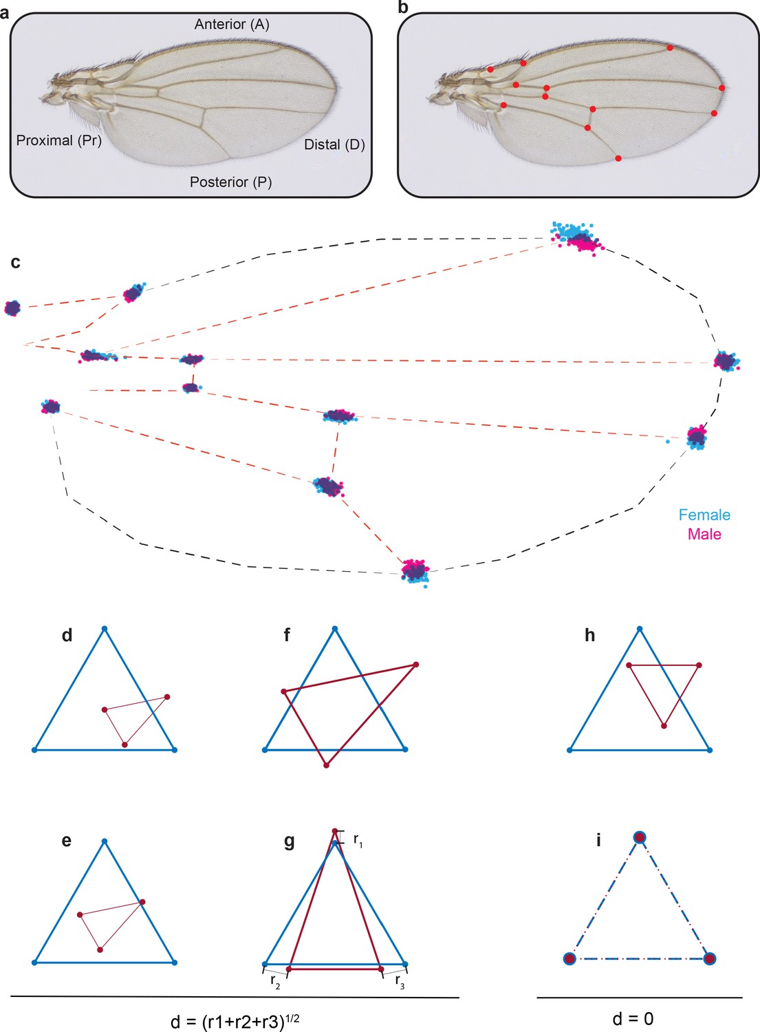
Procrustes alignment of landmarks.
(a) Image of a Drosophila wing with axes labeled. (b) Image of a wing with the 12 standard landmarks used in Procrustes analysis. (c) Positions of landmarks of outbred wildtype male and female wings after Procrustes alignment. (d–g) In order to explain Procrustes alignment, we use a simple example with two triangles of different size, shape, and orientation (d). (e) The first step is to align their centroids. (f) The second step is to scale the two shapes to make them of equal area. (g) The last step is rotation to optimally align the shapes. (h, i) The simplest case is when the triangles have identical shape (h), and as a result, Procrustes alignment generates complete overlap of the vertex landmarks (i).
Figure 1—figure supplement 2
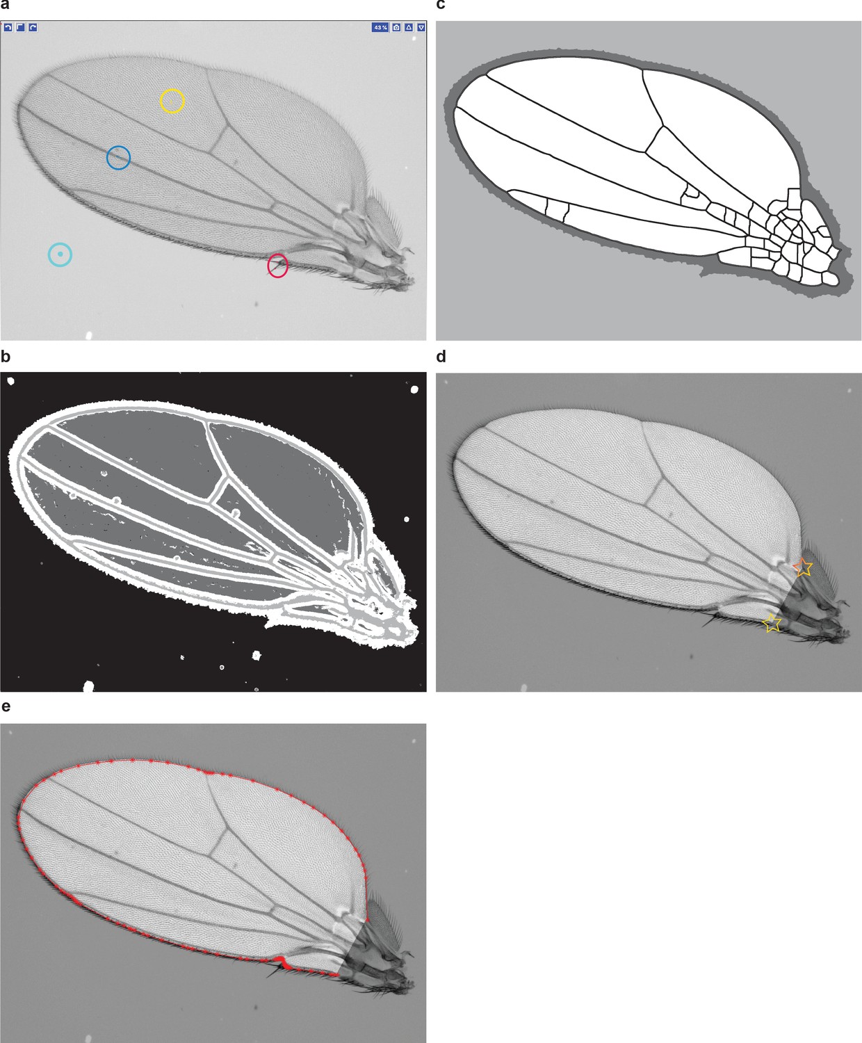
Wing boundary identification.
(a) An example of a training layer for Ilastik classification. The model has four layers: wing bulk (yellow), veins (blue), bristles (red), and background (cyan). (b) Output of Ilastik. (c) Cleaning the layers is required for boundary identification. Therefore, spurious veins appearing on the mask are not a concern. (d) Example of a wing image after the wing boundary has been segmented and cleaned. The interior of the wing is unmasked, whereas pixels outside of the wing have been uniformly dimmed. This is done merely for demonstration purposes and is not part of the pipeline. Note that there are two morphological landmarks marked with stars: the alula notch and humeral break. The complete boundary segmentation draws a line between them and excludes the hinge. (e) A polygon with vertices (red points) that we use to represent the wing boundary for conformal mapping.
Figure 1—figure supplement 3
Structure and form of the Drosophila wing.
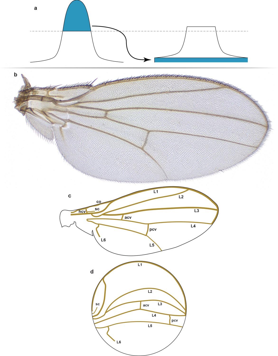
(a) Contrast-limited adaptive histogram equalization (CLAHE). The part of the histogram that exceeds the clip limit redistributes equally among all histogram bins. In contrast to ordinary histogram equalization, CLAHE is applied locally to patches of the image (tiles), and therefore uses several local histograms to redistribute the lightness values of the image. Thus, it is suitable for edge enchantment and improvement of the local contrast in every tile. (b) A representative example of a male right wing from the outbred wildtype population that was imaged. (c) Schematic of the wing structure. The longitudinal veins include L1, L2, L3, L4, L5, and L6. The cross-veins include the anterior (acv), humeral (hcv), and posterior (pcv) cross-veins. Other veins include the costa (co) and subcosta (sc) veins. (d) Schematized conformal map of wing in panel (c) showing the approximate locations and paths of the various veins.
Figure 1—figure supplement 4
Conformal map representation.
(a–c) An example of the conformal map between a disc (a), a triangle (b), and a square (c) showing polar grids. (d–f) An example of the conformal map between a square (d), a disc (e), and for the exponential function w = exp(z) (f) showing Cartesian grids. In all cases, grid lines remain perpendicular to each other. (g, h) An irregular polygon (g) is mapped onto a unit disc (h). The polygon’s vertices (black dots) map to the disc boundary as shown. (i) An example of the image mapping from the wing onto the disc. (j–l) We mapped polar and Cartesian grids of the same wing for demonstrational purposes. We must define a pre-image of the origin of the wing (j, k, left), that is, the point that will be mapped onto the center of the disc (j, k, right). For the Drosophila wing, it is the black dot at the intersection of the ACV and L4 veins. (l) The unit disc has an automorphism, that is, a map onto itself. It means that we can keep the boundary the same, but we still can rotate the disc and we can move the origin of the disc, as shown.
Figure 2 with 3 supplements
Comparison of Procrustes and landmark-free phenotyping.
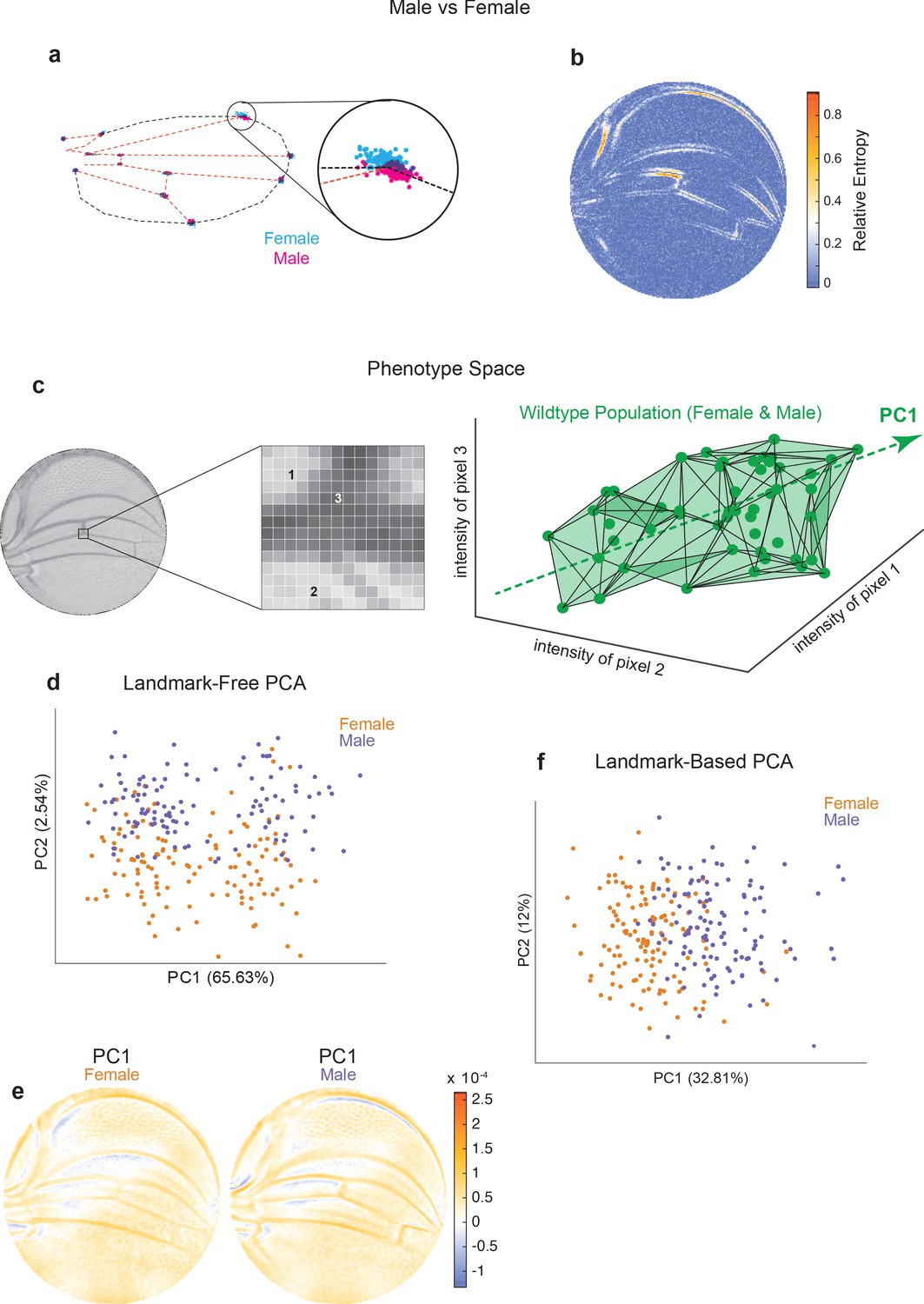
(a, b) Variation between ensembles of male and female wings from the outbred wildtype population. (a) Procrustes analysis with inset showing the landmark where L1 and L2 veins intersect. (b) Per-pixel symmetrized Kullback–Leibler divergence in landmark-free analysis detects variation along veins, undetected by landmark-based analyses. (c) The dimensions of phenotype space comprise individual pixels. Three such pixels are randomly selected here to show their 3D phenotype space. An ensemble of wings are points in this space. The direction of largest variation in the space is identified by principal component analysis (PCA) as PC1. (d) Landmark-free PCA of the outbred wildtype population reveals a novel dominant direction of variation orthogonal to sex-specific variation. Sex-specific variation aligns with PC2. (e) Pixel alignment with PC1 analysis shown in panel (d), showing vein position variation aligns with PC1. (f) Procrustes-based PCA of the same ensemble analyzed in panel (d). PC1 only detects the sex-specific variation.
Figure 2—figure supplement 1
Accounting for the variation in wings.
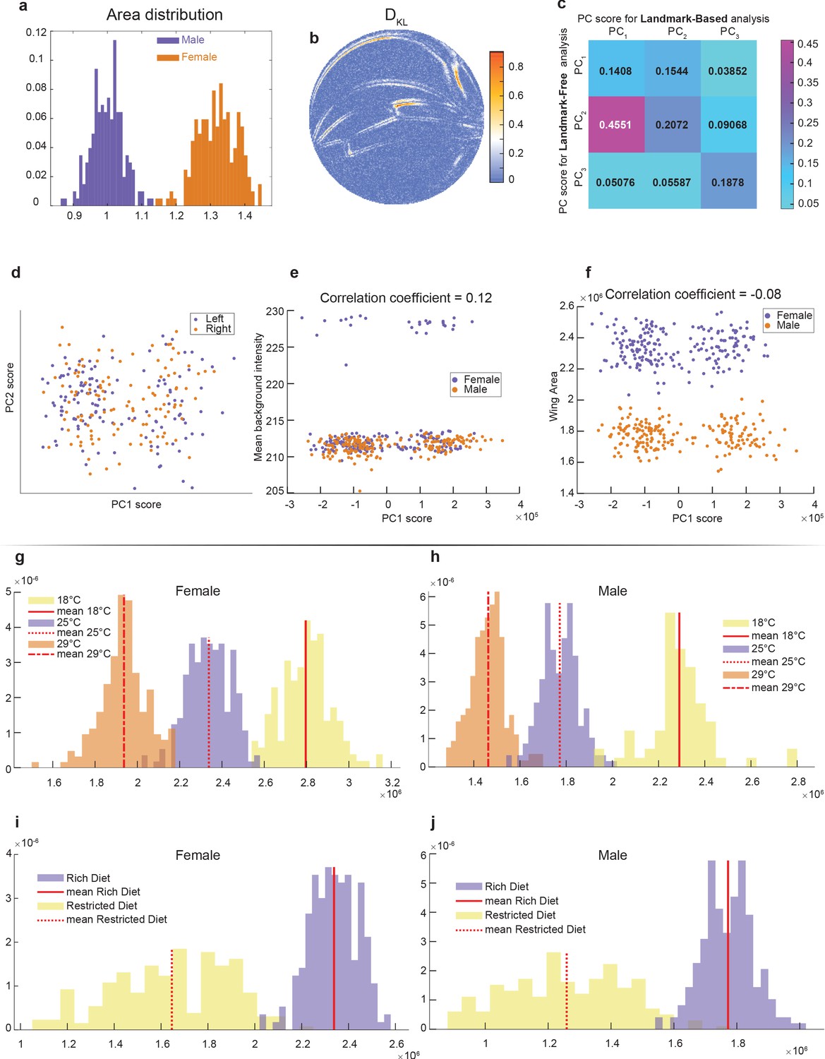
(a) Area distribution of wings from outbred wildtype females and males raised on a standard rich diet at 25°C. (b) Kullback–Leibler divergence between the male and female ensembles with single-pixel resolution. It was computed using second-nearest-neighbor Kozachenko–Leonenko estimator. (c) Cross-correlation between scores for principal component (PC) derived from Procrustes (landmark-based) and landmark-free analysis. Strong correlation is only observed between PC1 of the Procrustes analysis and PC2 of the landmark-free analysis. Both were identified as the axis pertaining to sexual dimorphism. This further highlights that the novel direction identified by our landmark-free analysis is absent in the principal component analysis (PCA) of the Procrustes analysis. (d–f) PCA plots of outbred male and female wings by landmark-free analysis, visualizing wing handedness (d), background pixel intensity (e), and area of the wing (f). Neither handedness, background intensity, nor wing area are the origins of the dominant mode observed in the landmark-free analysis. (g, h) Distribution of wing area for males (g) and females (h) at 18°C, 25°C, and 29°C. (i, j) Distribution of wing area for males (i) and females (j) raised on rich or restricted diets.
Figure 2—figure supplement 2
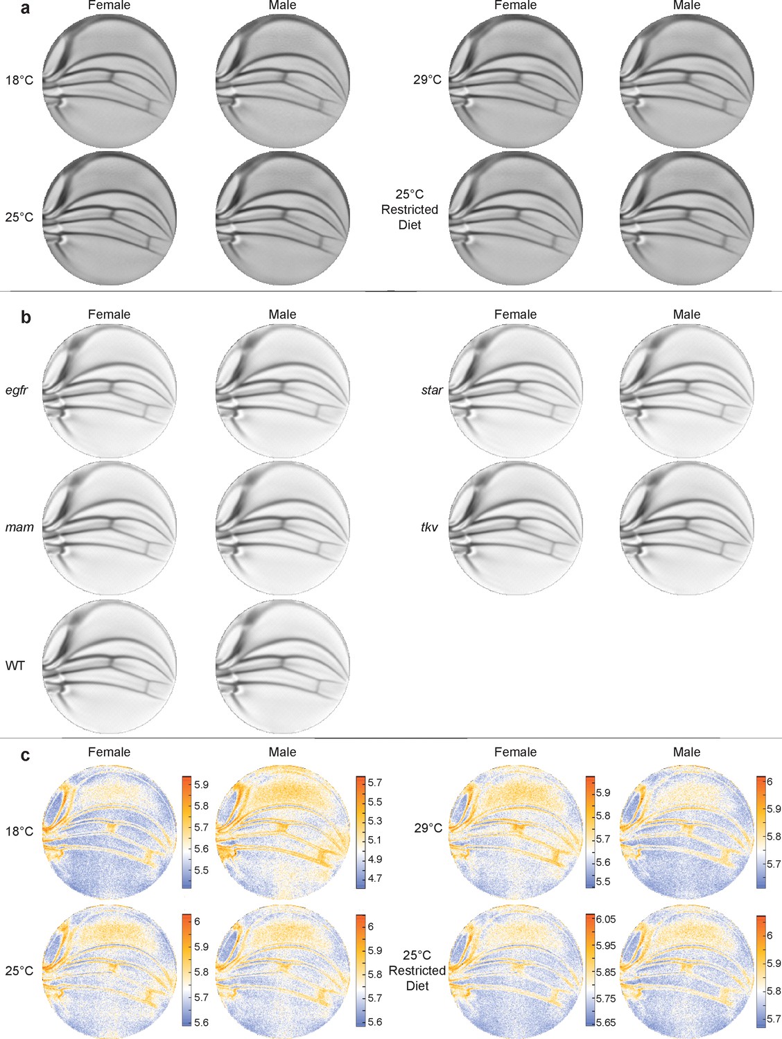
Mean wing conformal maps from animals raised under different conditions or with different genotypes.
(a) Mean wings from ensembles of outbred wildtype (WT) male and female flies raised under the diet and temperature conditions, as indicated. Differences between mean wings are subtle and require quantitative analysis to discern differences. (b) Mean wings from the ensembles of WT and heterozygous mutants, as indicated. Note how qualitatively similar the mean wings are to one another by eye. (c) Per-pixel variation within the ensembles shown in panel (a) is displayed as entropy plots. The Kozachenko–Leonenko second-nearest-neighbor estimator was used.
Figure 2—figure supplement 3
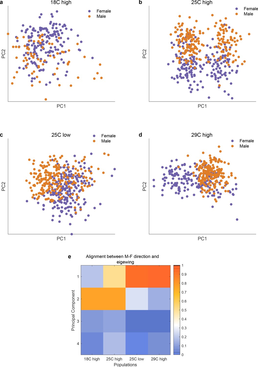
Alignment of axis of sexual dimorphism rotates as a function of environmental stress across 4 different conditions.
(panels a-d) and the degree of alignments betweeen the axis of sexual dimorphism and the top principal components of each of the conditions (panel e). As is apparent in the scatter plots in panels a-d and the quantitative assessment in panel e, the axis of sexual dimorphism rotates into the top principal component in stressed conditions.
Figure 3 with 4 supplements
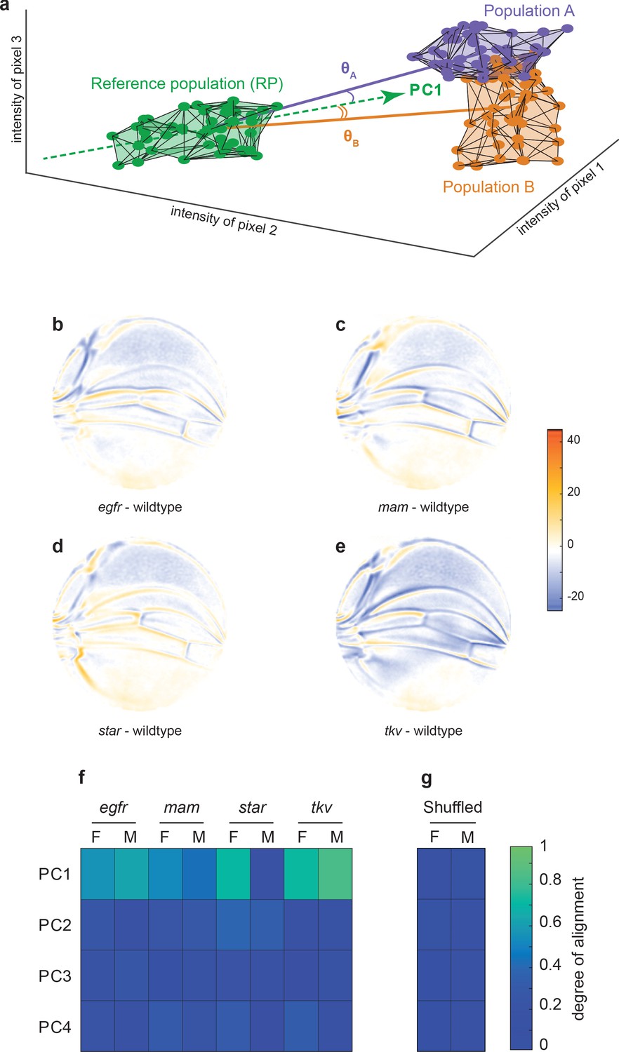
Variational analysis of genetic mutants.
(a) Schematic of hypothetical 3D phenotype space, with each cloud of points representing wings from an ensemble subject to a different treatment or condition. The principal component (PC)1 vector for each cloud of points can be independently calculated. The vectors joining the centroids of any two clouds of points can also be calculated. The angles between the direction of maximal variation (PC1) of the reference population and the directions from the reference to test ensembles are measured (θA and θB). (b-e) Per-pixel intensity difference between each mutant and the wildtype reference as measured at the center of each point cloud. Negative values are when mutant pixel intensity is smaller than wildtype, and positive values are when mutant pixel intensity is larger. Comparison between wildtype and egfr (b), mam (c), Star (d), and tkv (e) ensembles. (f) The cosine of the angle between the directions of PC1–PC4 of the outbred wildtype population, and the directions of the vectors connecting the wildtype and mutant populations. M and F refer to male and female groups, respectively. (g) The cosine of the angle when the wildtype and mutant populations analyzed in panel (f) are shuffled but the sexes are not. Shuffling leads to little or no alignment of mutant vectors with any PC.
Figure 3—figure supplement 1
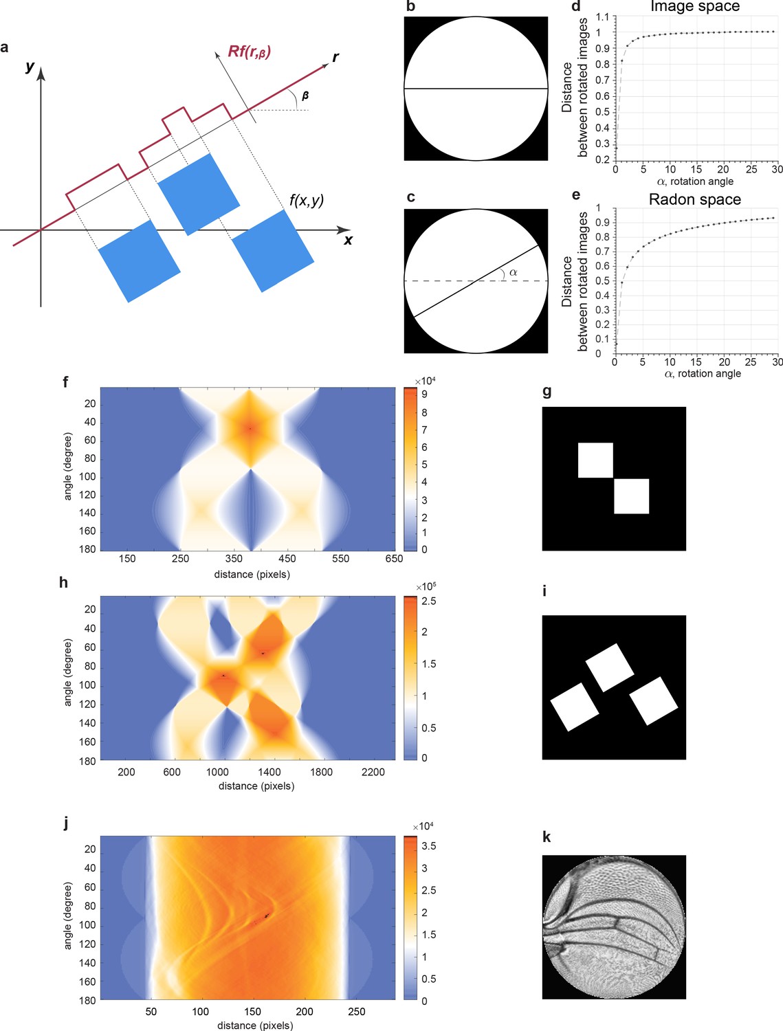
Radon transformation.
(a) A Radon transform maps f on the (x, y) domain to Rf (r, β) on the (r, β) domain. The function f is equal to 255 in the blue squares and 0 otherwise. This simulates an 8-bit image containing only the minimum and maximum intensity values. A transformation of f onto a line with an angle of β generates values of Rf that vary as a function of r, the position along the line. Note that Rf values are not binary, unlike the original image. The range and resolution of Rf values is much greater. (b–e) How a Radon transform makes line variation easier to detect. The reference image is a simple horizontal black line on the white disc (b), while the test image used for comparison is the same line but rotated by angle α (c). The angle is systematically rotated in the test image, and the distance between test and reference images is measured and plotted. Distance is normalized to the distance between the reference image and the test image rotated by 90°. This analysis was performed in image space (d) and Radon space (e). Note how distance in image space is switch-like in dependence on angle as opposed to the dependence in Radon space. (f–i) Example binary images before Radon transformation (g, i). Radon transforms of the images showing Rf values as heat maps on the plots of distance r in pixel units and angle in degrees (f, h). (j, k) A contrast-enhanced (contrast-limited adaptive histogram equalization [CLAHE]) wing image conformally mapped to a disc (k). Rf values are shown as a heat map on the plot of distance r in pixel units and angle in degrees (j).
Figure 3—figure supplement 2
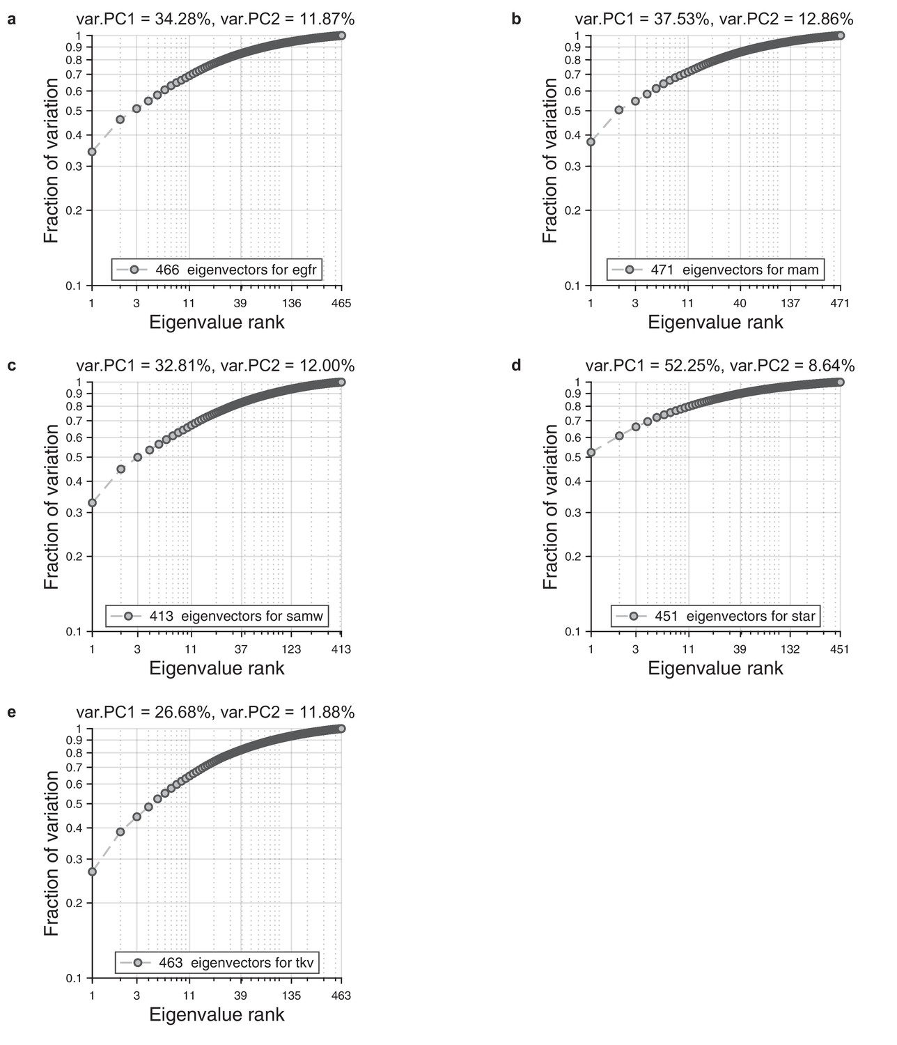
Eigenvalue spectrum in wings.
For each ensemble of wings, we performed alignment to the reference wing and Radon transformation. For each population, we performed principal component analysis on a single population. As a result, we obtained spectrum of the eigenvalues. We present cumulative normalized sum for these spectrums. (a) Eigenvalue spectrum for egfr mutant. (b) Eigenvalue spectrum for mam mutant. (c) Eigenvalue spectrum for wildtype. (d) Eigenvalue spectrum star mutant. (e) Eigenvalue spectrum tkv mutant.
Figure 3—figure supplement 3
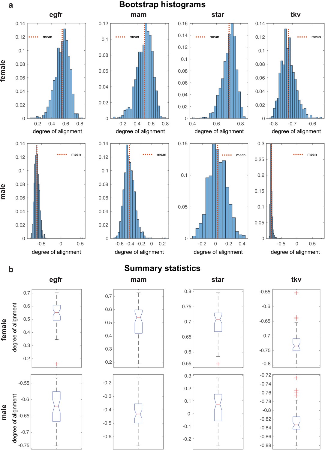
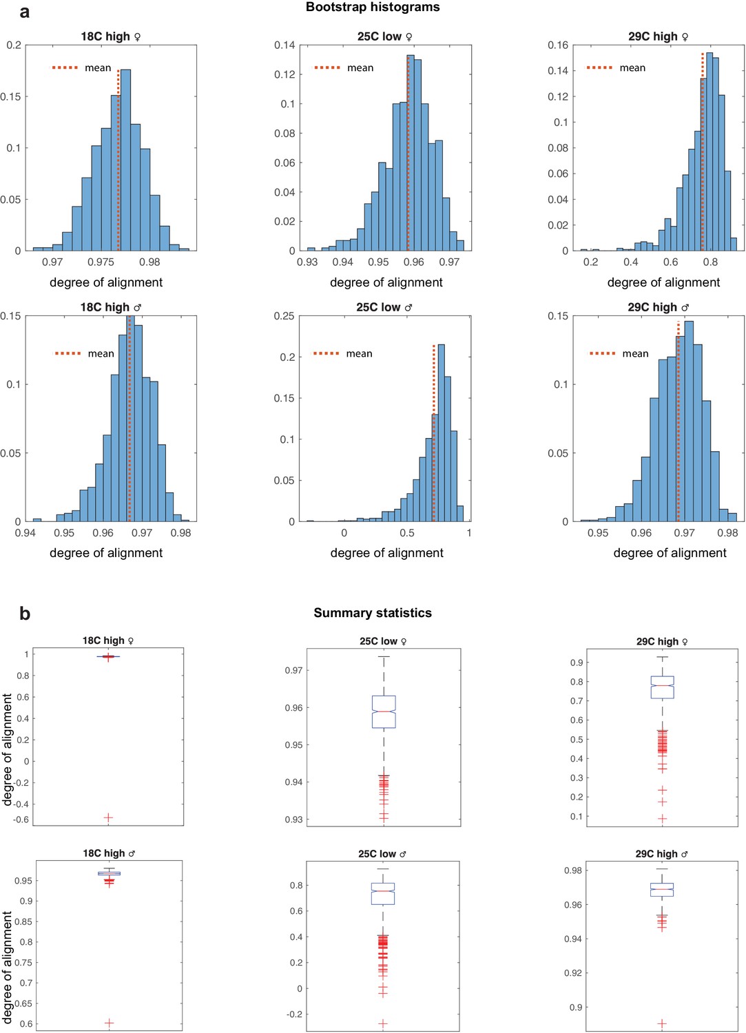
Bootstrap for genetic ensemble.
(a) Bootstraped distributions for the degree of alignments in mutant conditions, for males and females. (b) Box whisker plots summarizing histograms in panels a. Alignment distributions of different mutants.
Figure 3—figure supplement 4
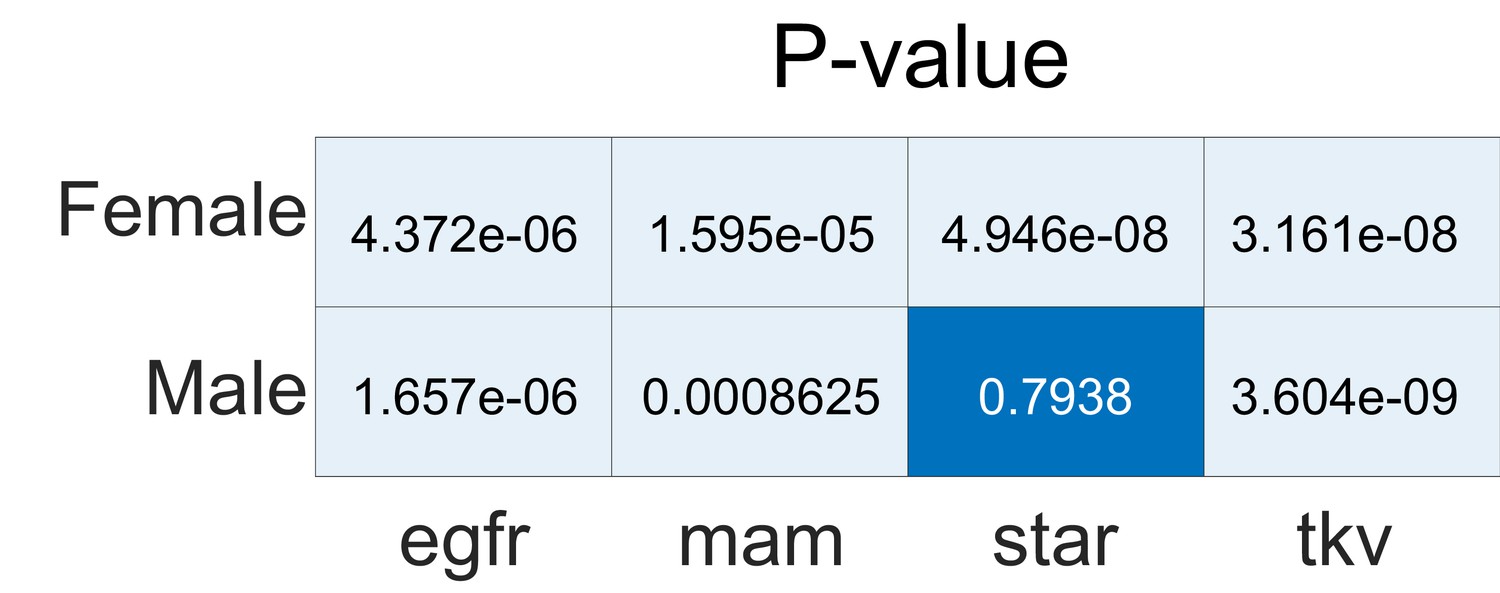
Statistical significance (p-values) of alignments in genetic analyses relative to a shuffled label null distribution.
Figure 4 with 4 supplements

Variational analysis of environmental perturbations.
(a–c) Per-pixel intensity difference between wings from a test condition (described on left) and a reference condition (described on the right). Difference is measured at the center of each point cloud. Negative values are when test pixel intensity is smaller than reference, and positive values are when test pixel intensity is larger. Comparison between wings from 18°C and 25°C (a), 29°C and 25°C (b), and restricted vs. rich diet (c) treatment. (d) The cosine of the angle between the directions of principal component (PC)1–PC4 of the outbred wildtype population, and the directions of the vectors connecting the populations raised under different temperature and diet conditions. M and F refer to male and female groups, respectively. (e) The cosine of the angle when the treated populations analyzed in panel (d) are shuffled but the sexes are not. Shuffling leads to little or no alignment of vectors with any PC.
Figure 4—figure supplement 1
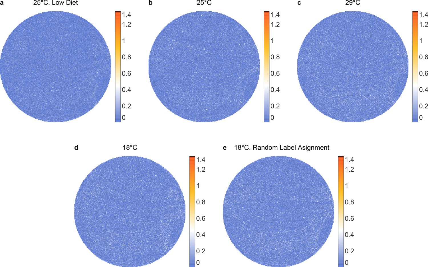
Kullback–Leibler divergence between left and right wings for each populations of female flies.
(a) 25°C, low diet, (b) 25°C, (c) 29°C, (d) 18°C, and (e) 18°C random left-right label assignment for population of 18°C.
Figure 4—figure supplement 2
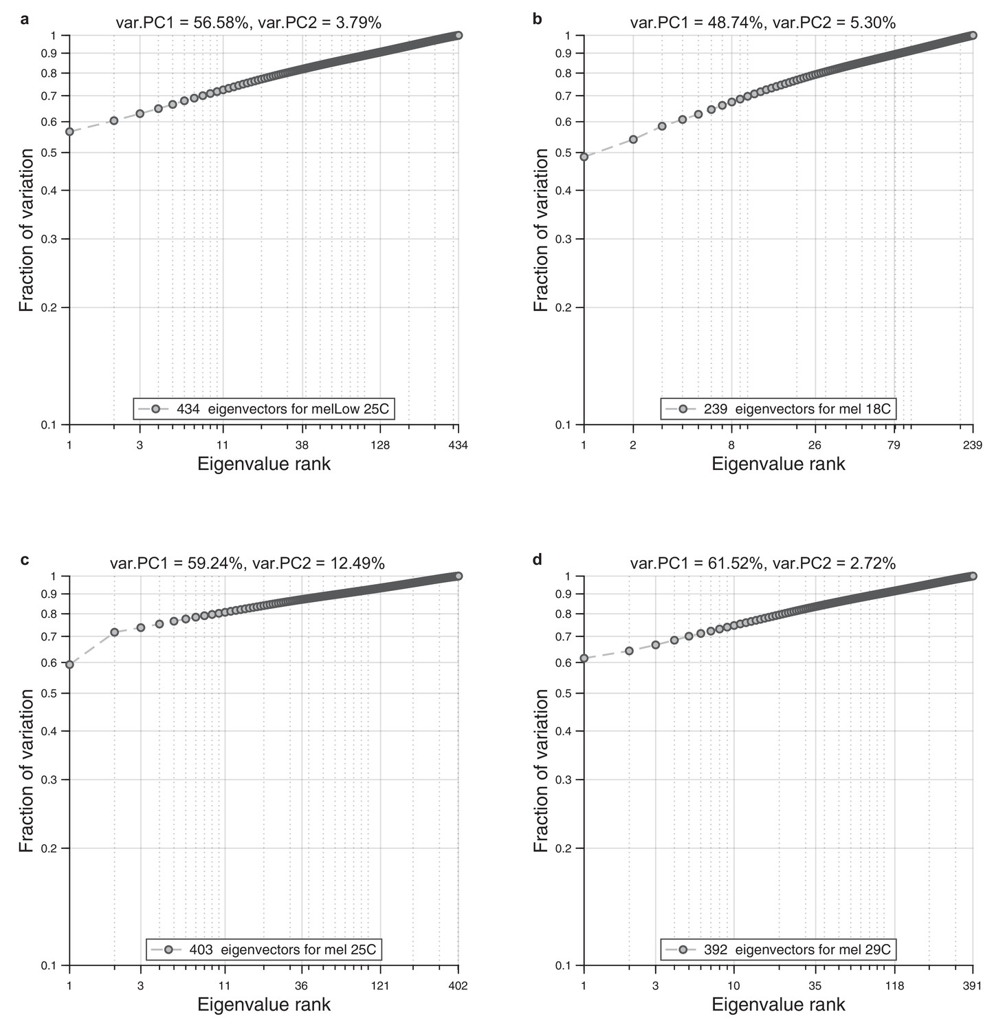
Eigenvalue spectrum in wings.
For each ensemble of wings, we performed alignment to the reference wing and Radon transformation. For each population, we performed principal component analysis on a single population. As a result, we obtained spectrum of the eigenvalues. We present cumulative normalized sum for these spectrums. (a) Eigenvalue spectrum for low diet and normal temperature (25°C). (b) Eigenvalue spectrum for rich diet and low temperature (18°C). (c) Eigenvalue spectrum for rich diet and normal temperature (25°C). (d) Eigenvalue spectrum for rich diet and high temperature (29°C).
Figure 4—figure supplement 3
Bootstrap for environmental ensembles.
(a) Bootstraped distributions for the degree of alignments for the environmental ensembles. Variability is far greater in the stressed populations at 29c and low diet. (b) Box whisker plots summarizing histograms in panels a. Alignment distributions of environmental ensembles.
Figure 4—figure supplement 4
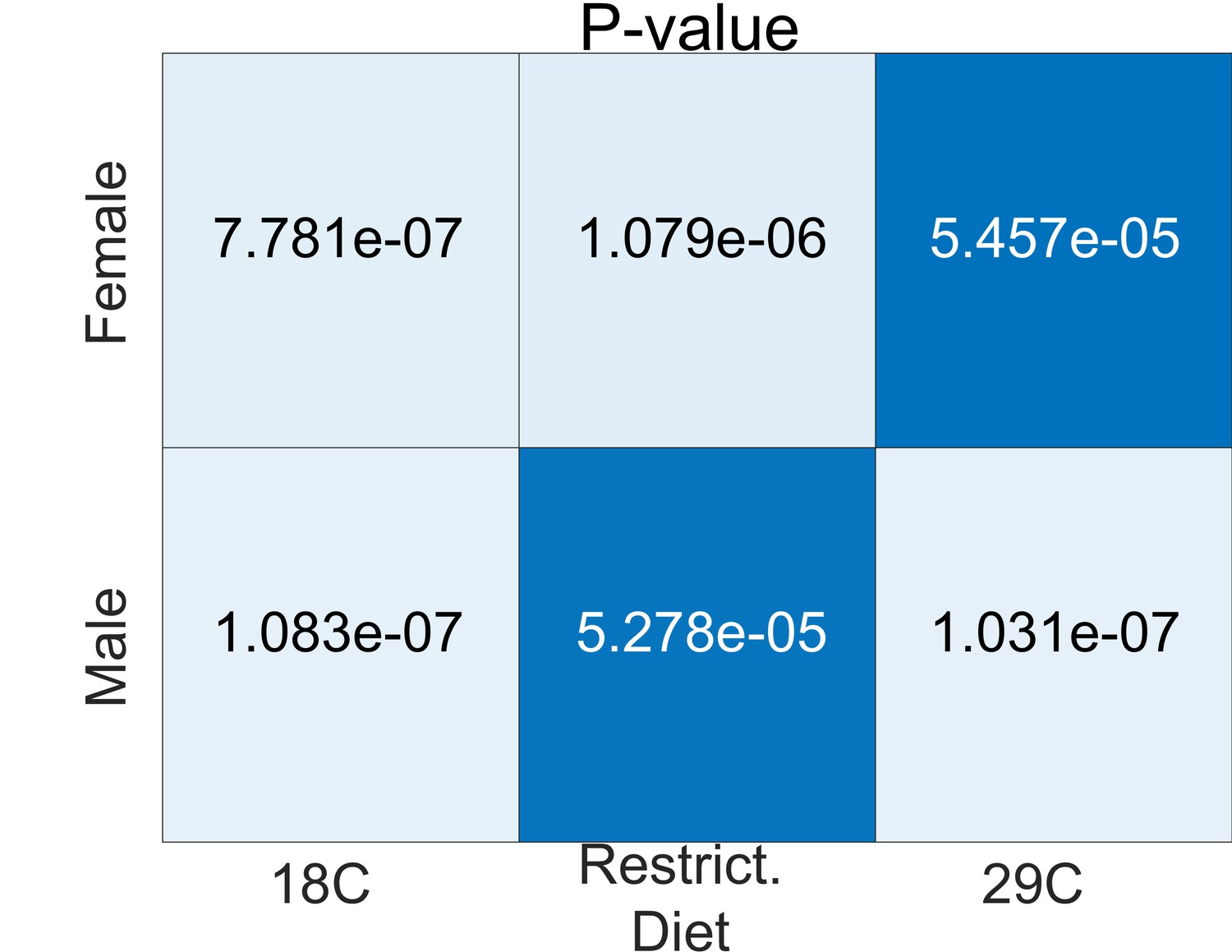
Statistical significance (p-values) of alignments in environmental analyses relative to a shuffled label null distribution.
Figure 5 with 3 supplements
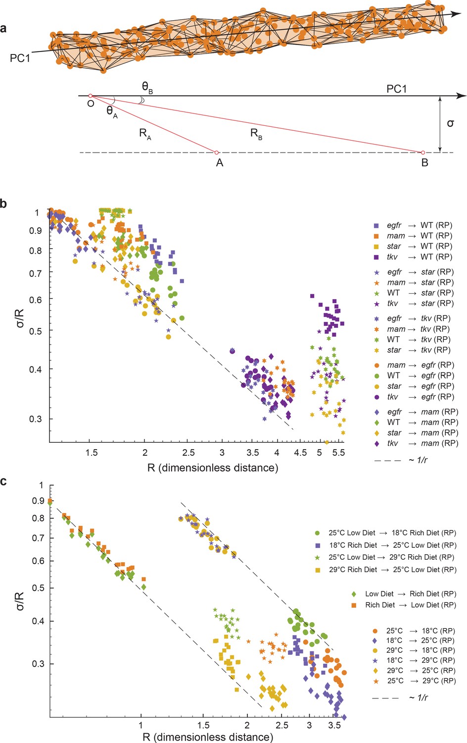
Geometric analysis of dominant variational mode.
(a) Schematic of a data manifold with a single dominant linear direction of variation, embedded in high-dimensional phenotype space. Variation orthogonal to the dominant direction is visualized with a characteristic scale, σ. In the presence of such a data manifold, the angle between the dominant direction of a reference population, principal component (PC)1, and the centroid-to-centroid vector connecting any two populations is predicted to decrease as a function of R, the length of the centroid-to-centroid vector. (b, c) The angle between the direction of maximal variation (PC1) in a reference population (RP) and the centroid-to-centroid vector connecting the RP and a second population as indicated. This is shown as a function of R, the distance between them. Samples are bootstrapped to indicate the in-sample variance, with each bootstrap represented by a point. Both in the mutant/wildtype (WT) (b) and environmental (c) ensembles, alignment grows as a function of distance, indicative of a single dominant direction in the data manifold. The dotted lines represent the relationship between σ /R versus R if sigma was a constant.
Figure 5—figure supplement 1
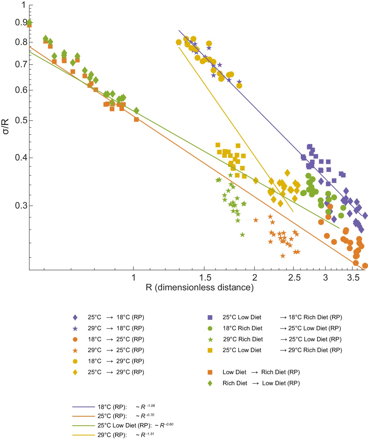
Geometric analysis of dominant mode.
We observe the expected increase in alignment between directions of variation and directions connecting distinct populations. We fitted power laws to the experimental value of the trigonometric quantity . One-dimensional structure may be cylinder (if ) or a cone-like structure if . An exact cylinder case means that 'noise' is constant along the axes, while other power means that 'noise' changes with distance in this space.
Figure 5—figure supplement 2
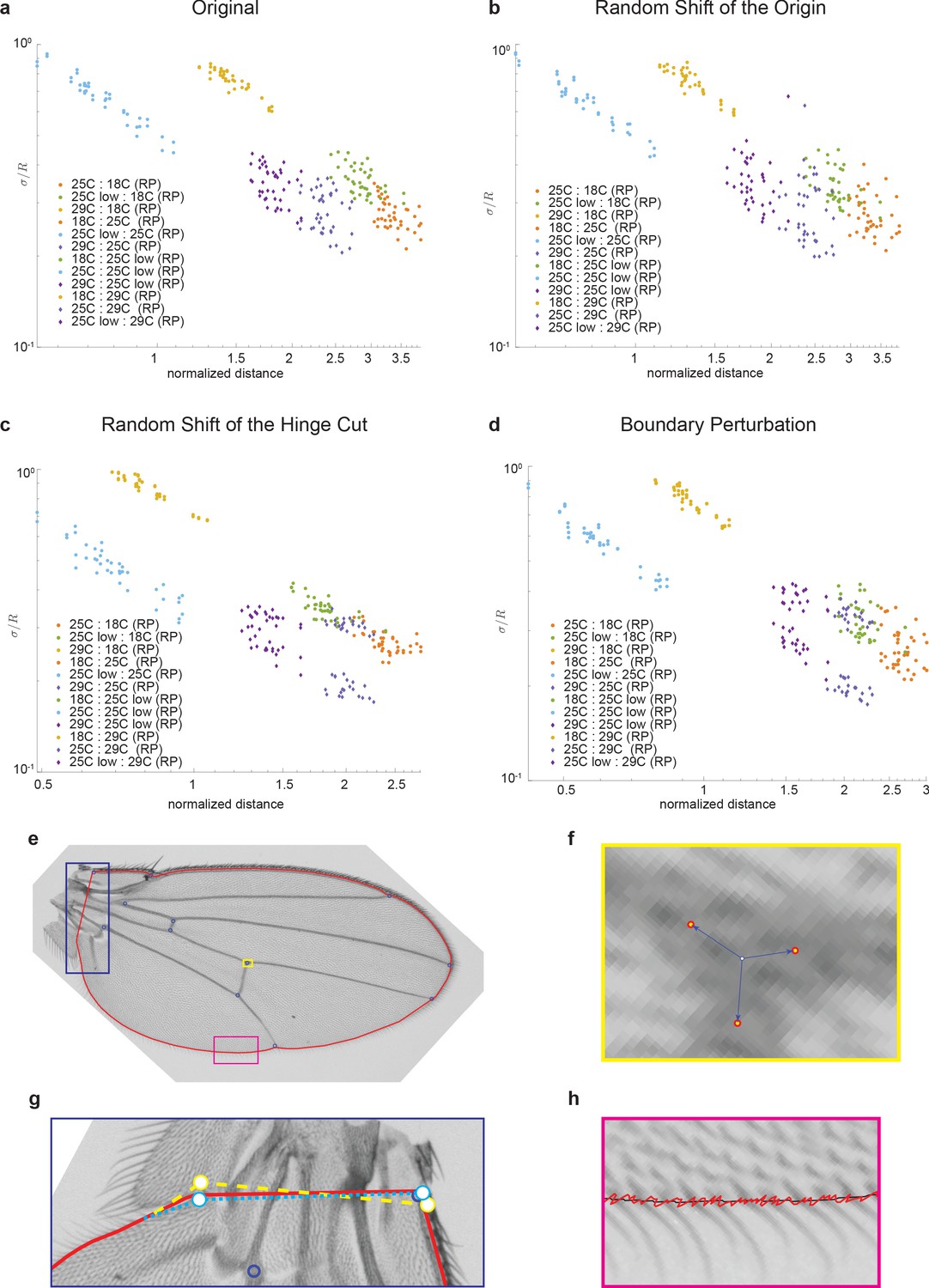
Robustness of manifold geometry to perturbations in image analysis pipeline.
In each panel, sigma/R vs. R is plotted. (a) Original data, (b) random perturbation to location of origin, (c) random shift of hinge cut points, and (d) boundary perturbations. The schematics in panels (e–h) provide a visual representation of the nature of perturbations explored.
Figure 5—figure supplement 3
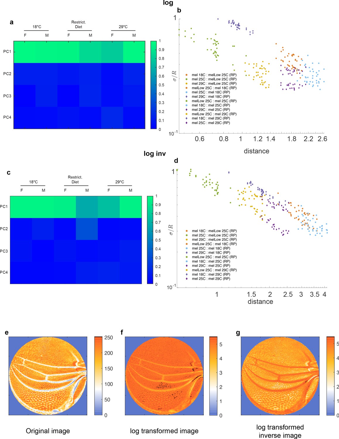
Degree of alignment and analysis of global geometry of (a, b) log-transformed data and (c, d) log-transformed inverse data.
Representative images are included in (e–g).
Additional files
-
Supplementary file 1
Description of inbred stock lines.
- https://cdn.elifesciences.org/articles/66750/elife-66750-supp1-v2.xlsx
-
Supplementary file 2
Crossing scheme.
- https://cdn.elifesciences.org/articles/66750/elife-66750-supp2-v2.xlsx
-
Transparent reporting form
- https://cdn.elifesciences.org/articles/66750/elife-66750-transrepform-v2.docx
Download links
A two-part list of links to download the article, or parts of the article, in various formats.
Downloads (link to download the article as PDF)
Open citations (links to open the citations from this article in various online reference manager services)
Cite this article (links to download the citations from this article in formats compatible with various reference manager tools)
Global constraints within the developmental program of the Drosophila wing
eLife 10:e66750.
https://doi.org/10.7554/eLife.66750


