Synaptic learning rules for sequence learning
- Institute for Theoretical Biology, Department of Biology, Humboldt-Universität zu Berlin, Germany
- Bernstein Center for Computational Neuroscience Berlin, Germany
- Einstein Center for Neurosciences Berlin, Germany
Figures
Figure 1
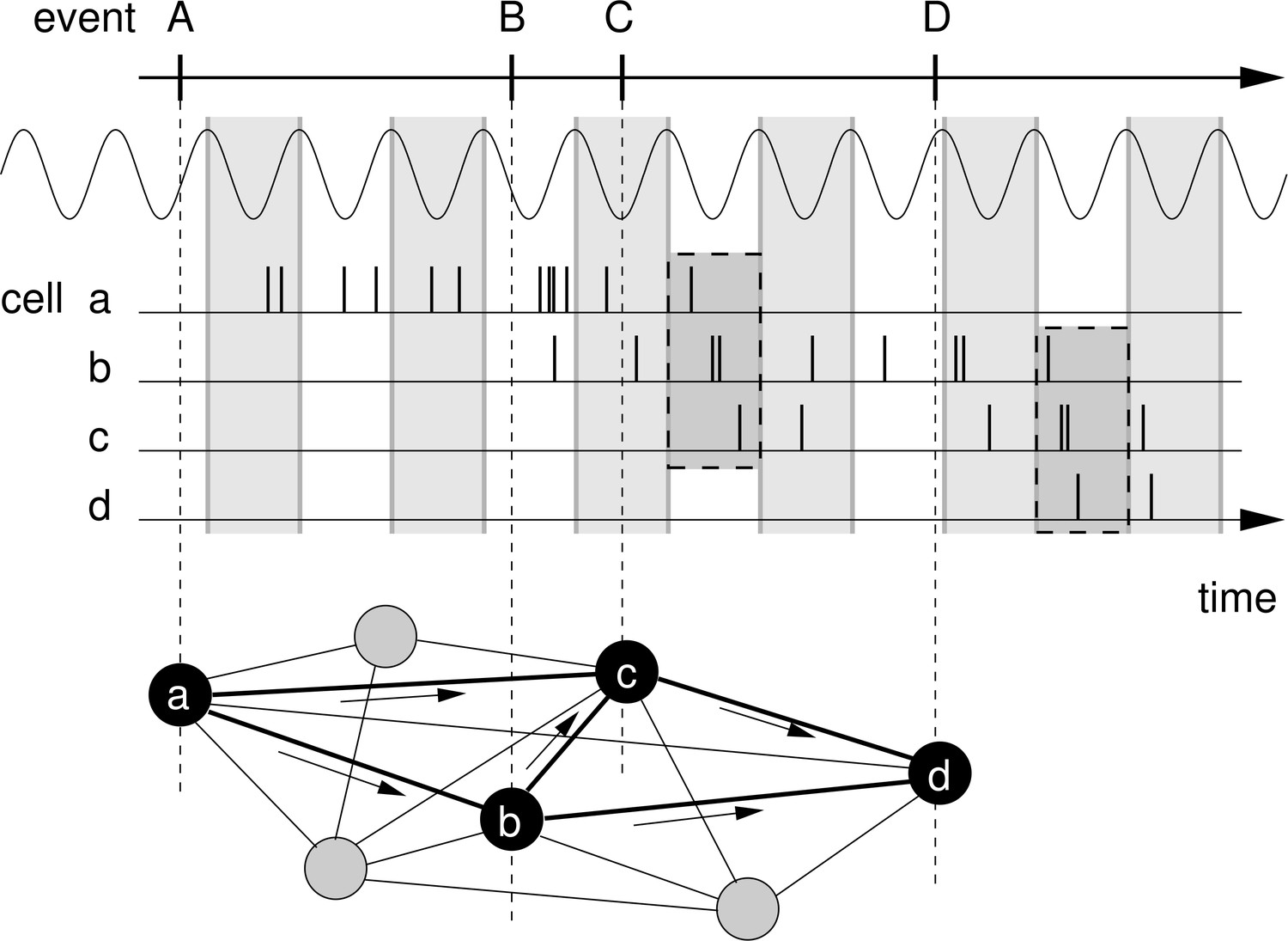
Rationale for temporal-order learning via phase precession.
Top: Behavioral events (A to D) happen on a time scale of seconds. Middle: These events are represented by different cells (a–d), which fire a burst of stochastic action potentials in response to the onset of their respective event. We assume that each cell shows phase precession with respect to the LFP’s theta oscillation (every second cycle is marked by a greay box). When the activities of multiple cells overlap, the sequence of behavioral events is compressed in time to within one theta cycle (two examples highlighted in the dashed, shaded boxes). Bottom: This faster time scale can be picked up by STDP and strengthen the connections between the cells of the sequence. Figure adapted from Korte and Schmitz, 2016.
Figure 2

Model of two sequentially activated phase-precessing cells.
(A) Oscillatory firing-rate profiles for two cells (solid blue and cyan lines). The black curve depicts the population theta oscillation. For easier comparison of the two different frequencies, the population activity’s troughs are continued by thin gray lines, and the peaks of the cell-intrinsic theta oscillation are marked by dots. Dashed lines depict the underlying Gaussian firing fields without theta modulation. (B) Phase precession of the two cells (same colors as in A). The compression factor describes the phase shift per theta cycle for an individual cell (). For the temporal separation of the firing fields and the theta frequency , the phase difference between the cells is . The dots depict the times of the maxima in (A). (C) Resulting cross-correlation for the two firing rates from (A). The solid red curve shows the full cross-correlation. The dashed line depicts the cross-correlation without theta-modulation. The gray region indicates small ( ms) time lags. (D) Same as in (C), but zoomed in. Note that the first peak of the theta modulation is at a positive non-zero time lag, reflecting phase precession. The dashed black curve shows the approximation of the cross-correlation for the analytical treatment (Materials and methods, Equation 17). (E) Synaptic learning window. The gray region indicates the region in which the learning window is large, and this region is also indicated in (C) and (D). Positive time lags correspond to postsynaptic activity following presynaptic activity. Parameters for all plots: s, Hz, s, ms, , , .
Figure 3
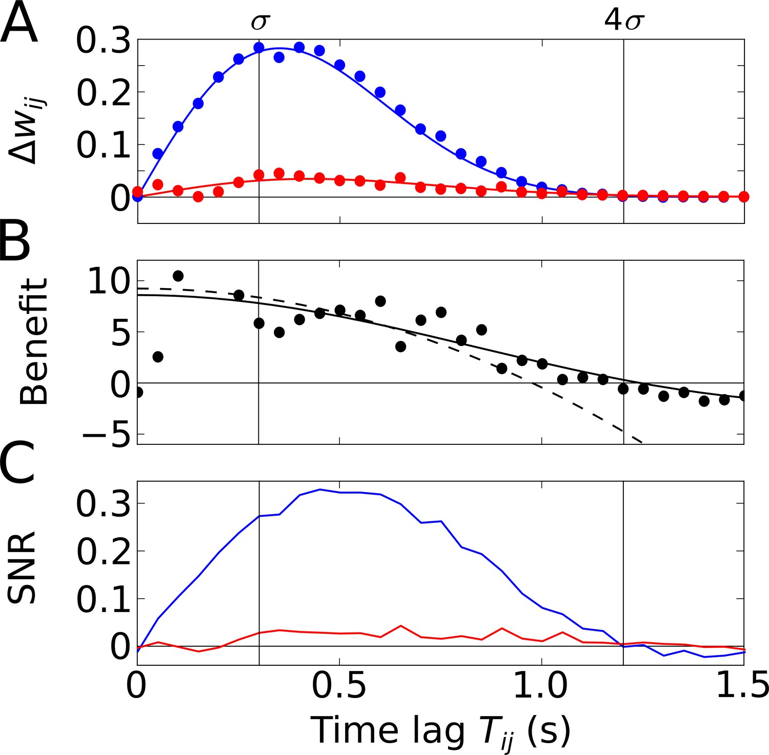
Temporal-order learning for narrow learning windows ().
(A) The average synaptic weight change depends on the temporal separation between the firing fields. Phase precession (blue) yields higher weight changes than phase locking (red). Simulation results (circles, averaged across 104 repetitions) and analytical results (lines, Equation 5) match well. The vertical lines mark time lags of and , respectively, where approximates the total field width. (B) The benefit of phase precession is determined by the ratio of the average weight changes of two scenarios from (A). The solid and dashed lines depict the analytical expression for the benefit (Equation 20) and its approximation for small (Equation 7), respectively. (C) Signal-to-noise ratio (SNR) of the weight change as a function of the firing-field separation . The SNR is defined as the mean weight change divided by the standard deviation across trials in the simulation. Colors as in (A). Parameters for all plots: Hz, s, ms, , , .
Figure 4
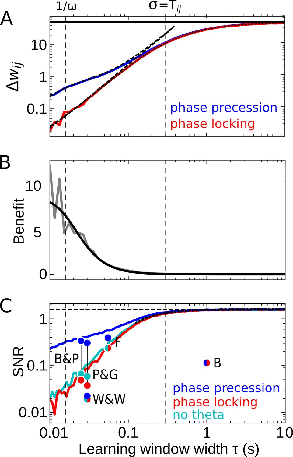
Effect of the learning-window width on temporal-order learning for overlapping fields (here: ).
(A) Average weight change as a function of width (for the asymmetric window in Equation 14) for phase precession and phase locking (colored curves). The solid black line depicts the theoretical maximum for large (, Equation 8). The dashed curves show the analytical small-tau approximations (Equation 5). The dotted curve depicts the analytical approximation for the ’no theta’ case (Equation A2-46 in Appendix 2). The vertical dashed lines mark s and the value of , respectively. (B) The benefit of phase precession is largest for narrow learning windows, and it approaches 0 for wide windows. Simulations (gray line) and analytical result (black line, small-tau approximation from Equation 20) match well. (C) The signal-to-noise ratio (SNR; phase precession: blue, phase locking: red, no theta: cyan) takes into account that only the asymmetric part of the learning window is helpful for temporal-order learning. For large , all three coding scenarios induce the same SNR. The horizontal dashed black line depicts the analytical limit of the SNR for large and overlapping firing fields (, Equation A1-17 of Appendix 1). The dotted black line depicts the analytical expression for the ’no theta’ case (Equation A2-48 in Appendix 2, the curve could not be plotted for s due to numerical instabilities). Dots represent the SNR for experimentally observed learning windows. The learning windows were taken from ‘B&P’, Bi and Poo, 2001: their Figure 1, ‘F’, Froemke et al., 2005: their Figure 1D bottom, ‘W&W’, Wittenberg and Wang, 2006: their Figure 3, ‘P&G’, Pfister and Gerstner, 2006: their Table 4, ‘All to All’, ‘minimal model’, and ‘B’, Bittner et al., 2017: their Figure 3D. For ‘B&P’, ‘F’, and ‘B’, the position of the dots on the horizontal axis was estimated as the average time constants for positive and negative lobes of the learning windows. Wittenberg and Wang modeled their learning rule by a difference of Gaussians — we approximated the corresponding time constant as 30 ms. For the triplet rule by Pfister and Gerstner, we used the average of three time constants: the two pairwise-interaction time constants (as in Bi and Poo) and the triplet-potentiation time constant. Parameters for all plots: s, Hz, s, , , . Colored/gray curves and dots are obtained from stochastic simulations; see Materials and methods for details.
Figure 5
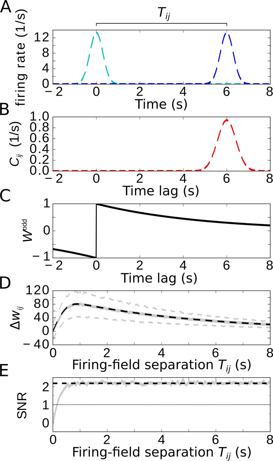
Temporal-order learning for non-overlapping firing fields using wide, asymmetric learning windows.
(A) Firing rates of two example cells with non-overlapping firing fields. (B) Cross-correlation of the two cells from (A). (C) Asymmetric learning window with large width ( s). (D) Resulting weight change for wide learning window and non-overlapping firing fields. The solid gray line depicts the average weight change. The dashed gray lines represent ±1 standard deviation across 1000 repetitions of stochastic spiking simulations. The analytical curve (dashed black line, Equation 9) matches the simulation results. (E) SNR of the weight change. Results of the stochastic simulations are shown by the gray curve. The SNR saturates for larger , which fits the analytical expectation (dashed black line, Equation 10). Parameters, unless varied in a plot: s, s, s, , .
Author response image 1
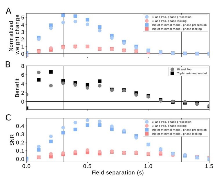
Comparison of pairwise and triplet STDP.
(A) Average weight change for the pairwise Bi-and-Poo learning rule (circles) and the minimal triplet model from Pfister and Gerstner, 2006 (squares). Bluish symbols represent phase precession, reddish symbols represent phase locking. Note that we have normalized the weight changes here (by the peak of the respective phase-locking curve) because the parameters A+ and A- differ in Bi and Poo (1998) as compared to Pfister and Gerstner, (2006) as they were fitted to different data sets. In Figure 3A in the manuscript we show the un-normalized weight change because we choose the learning-rate parameter 𝜇=1 for mathematical convenience. (B) Benefit of phase precession as defined in the manuscript (equation 6) for the Bi-and-Poo learning rule (circles) and the minimal triplet model (squares). (C) Signal-to-noise ratio for Bi-and-Poo learning rule and the minimal triplet model. Symbols and colors as in (A). We note that the results in B and C are independent of the value of the learning-rate parameter.
Additional files
Download links
A two-part list of links to download the article, or parts of the article, in various formats.
Downloads (link to download the article as PDF)
Open citations (links to open the citations from this article in various online reference manager services)
Cite this article (links to download the citations from this article in formats compatible with various reference manager tools)
Synaptic learning rules for sequence learning
eLife 10:e67171.
https://doi.org/10.7554/eLife.67171


