The solubility product extends the buffering concept to heterotypic biomolecular condensates
- R. D. Berlin Center for Cell Analysis and Modeling, University of Connecticut School of Medicine, United States
Figures
Figure 1 with 3 supplements
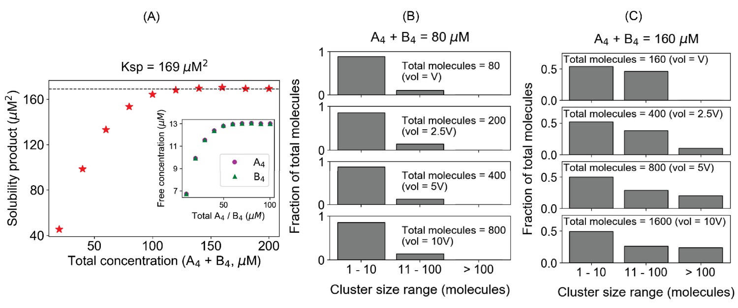
The solubility product constant corresponds to a threshold above which molecules distribute into large clusters.
These simulation results correspond to equal total concentrations of a heterotypic tetravalent pair of molecules with Kd for individual binding of 350 μM. (A) Product of the free monomer concentrations (solubility product) as a function of the total molecular concentrations. The black dashed line indicates the plateau, corresponding to the solubility product constant (Ksp), 169 µM2. Inset plot shows the change of free molecular concentrations of both tetravalent molecules with their respective total concentrations. Each data point is an average of steady-state values from 200 trajectories. In these simulations, we titrate up the molecular counts (200, 400, 600, ...., 2000 molecules, respectively), keeping the system’s volume fixed. (B, C) Distribution of cluster sizes with varying system sizes at two different total concentrations, 80 µM and 160 µM, respectively below and above the plateau in (A). The histograms show how the molecules are distributed across different ranges of cluster sizes.
-
Figure 1—source data 1
Source data for Figure 1.
- https://cdn.elifesciences.org/articles/67176/elife-67176-fig1-data1-v2.xlsx
Figure 1—figure supplement 1
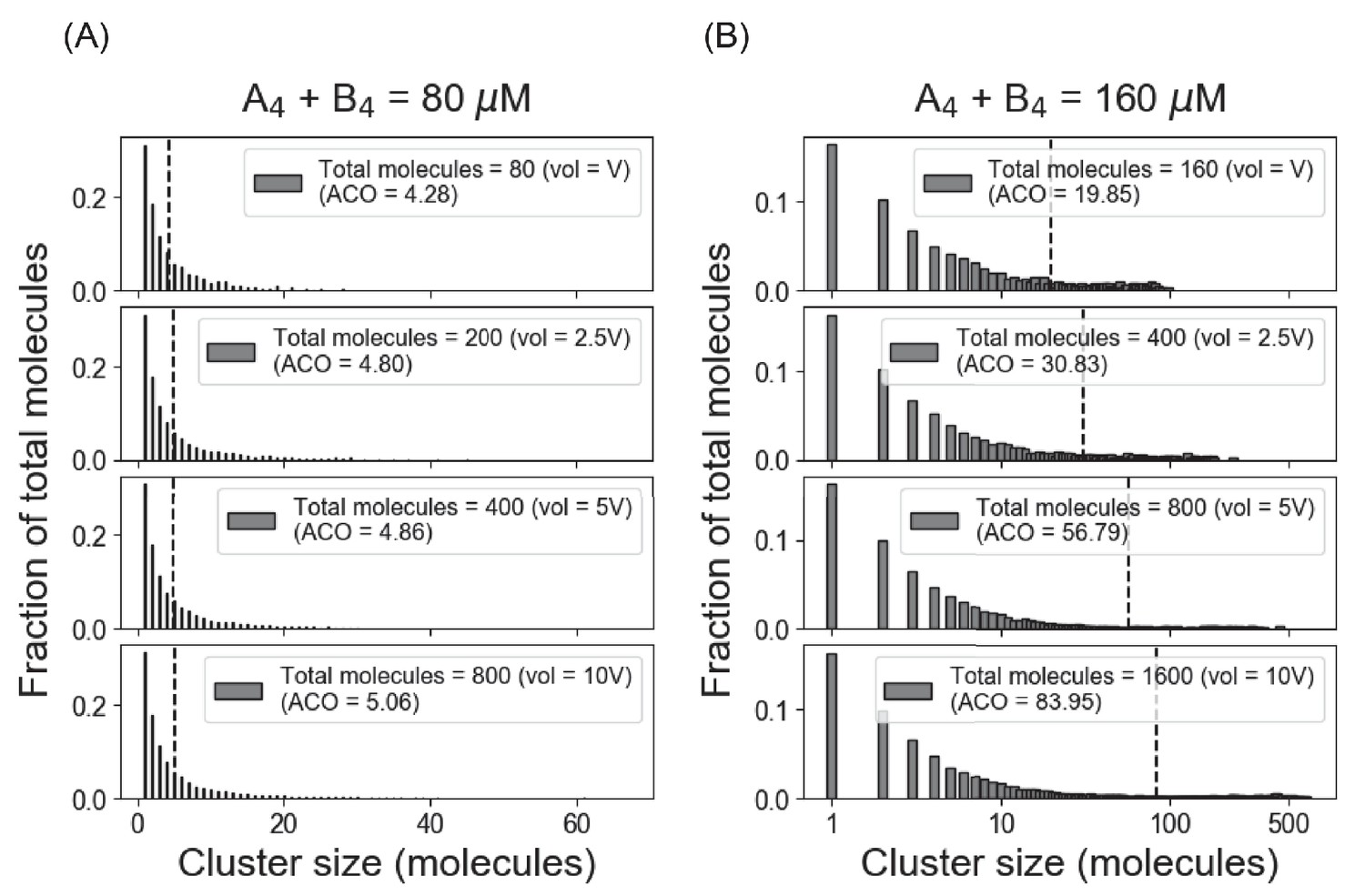
Full (unbinned) distributions of cluster sizes corresponding to Figure 1B, C.
(A) System shows similar cluster size distributions with varying volume and monomer counts as long as the total concentration (80 µM in this case) is below the threshold concentration (~ 120 µM for our A4 – B4 system). We term the mean of the distribution as average cluster occupancy (ACO) (Chattaraj et al., 2019), which is shown with dotted line in each case. (B) Above the threshold, the fraction of monomer is clamped at the Ksp, and larger clusters are formed as more molecules become available.
Figure 1—figure supplement 2
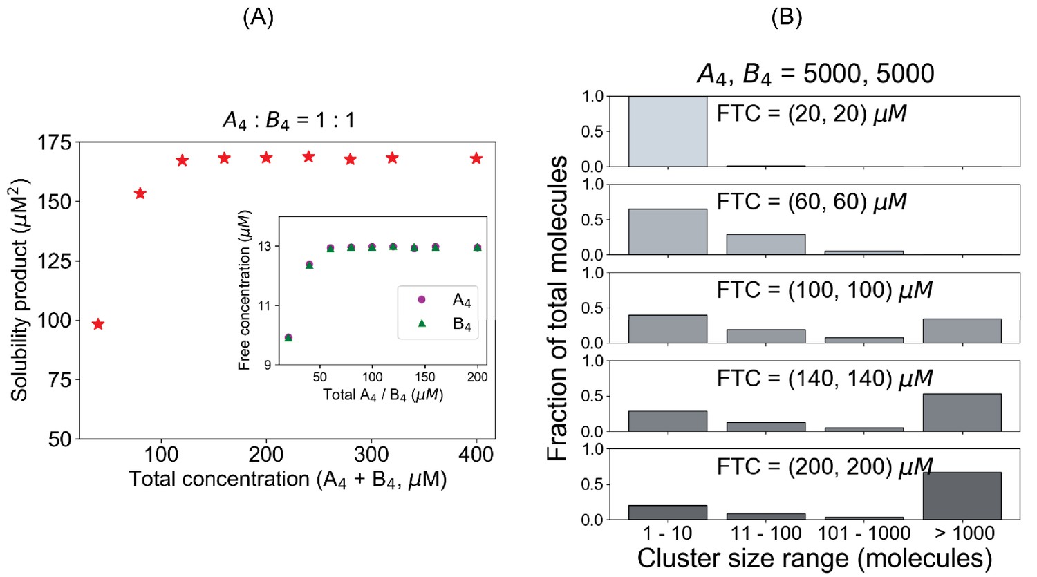
Pair of tetravalent heterotypic binders shows an identical Ksp even for a larger system.
(A) Solubility product profile and (B) cluster size distributions when we use A4 and B4 in equal stoichiometric amount. In all these cases, 5000 A4 and 5000 B4 molecules are kept fixed and we vary the volume to change the concentrations.
Figure 1—figure supplement 3
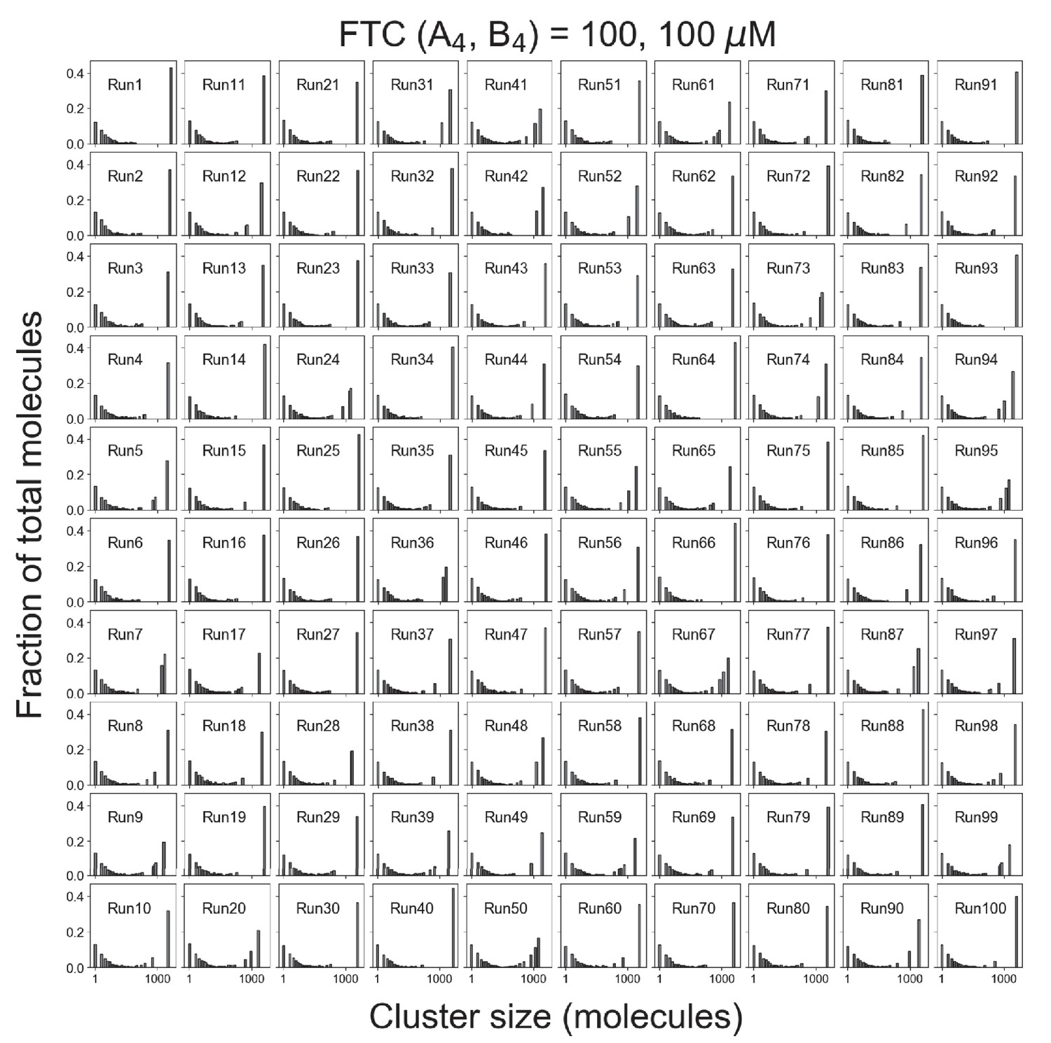
Distributions of cluster sizes for single trajectories.
Total molecules = 10,000 (5000 A4 and 5000 B4). Fixed total concentration (FTC) = 200 µM, which is above the phase transition threshold (~120 µM).
Figure 2 with 4 supplements
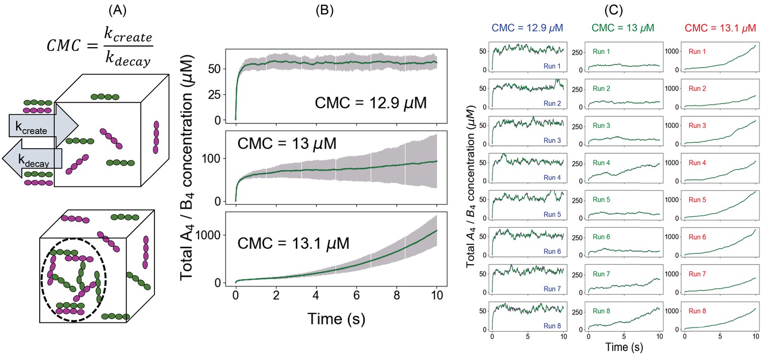
An alternative approach to quantify the phase transition boundary.
(A) Illustration of the clamped monomer concentration (CMC) approach. Both the molecules (A4 in magenta and B4 in green) can enter the simulation box with a rate constant kcreate (molecules/s) and exit with a rate constant kdecay (s-1). The ratio of these two parameters clamps the monomer concentration to (kcreate/kdecay). (B) Average time course (over 100 trajectories) of total molecular concentrations as a function of different CMCs. Error bars show the standard deviations across 100 trajectories. (C) Eight sample trajectories for different CMCs.
-
Figure 2—source data 1
Source data for Figure 2.
- https://cdn.elifesciences.org/articles/67176/elife-67176-fig2-data1-v2.xlsx
Figure 2—figure supplement 1
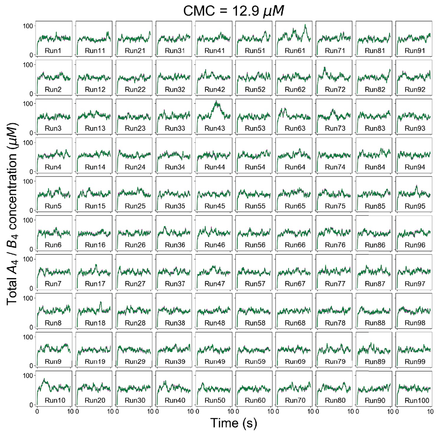
Individual trajectories of total molecular concentrations (A4 in magenta and B4 in green) at clamped monomer concentration (CMC) = 12.9 µM.
Figure 2—figure supplement 2
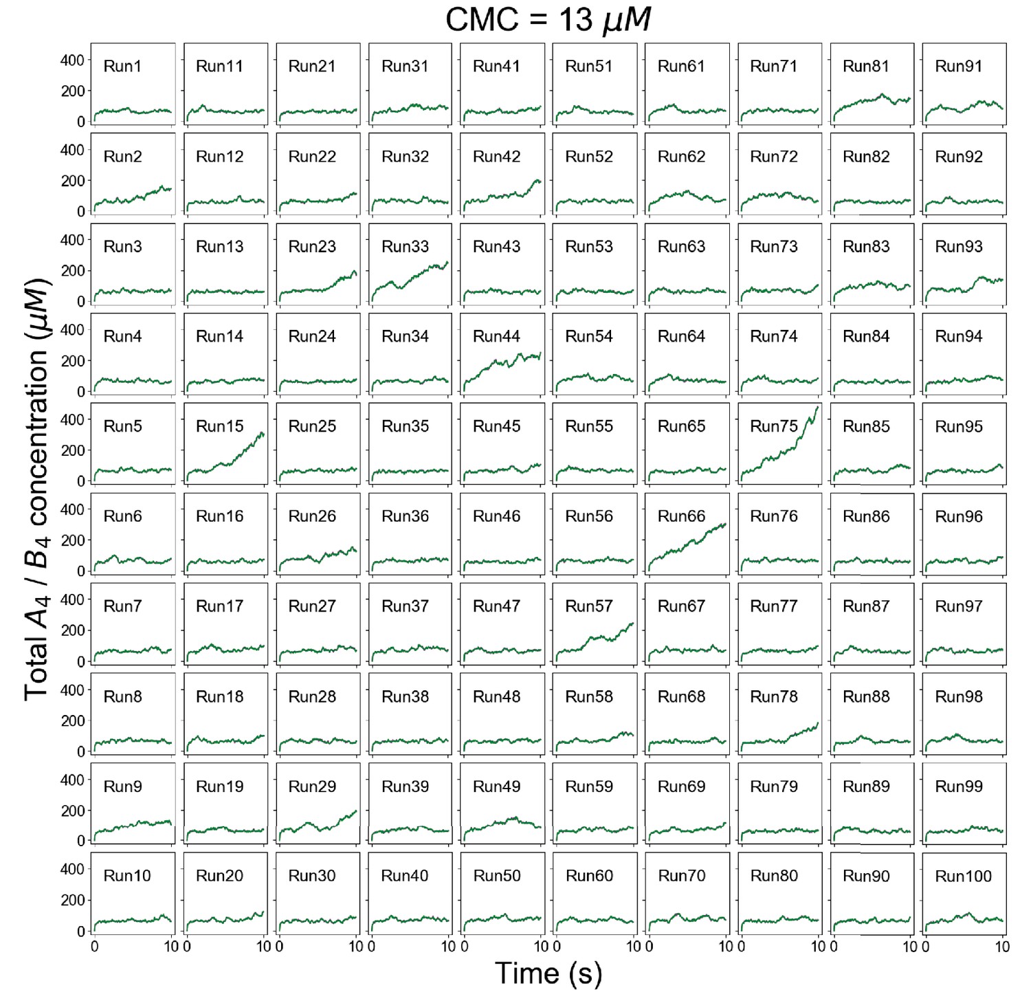
Individual trajectories of total molecular concentrations (A4 in magenta and B4 in green) at clamped monomer concentration (CMC) = 13 µM.
Figure 2—figure supplement 3
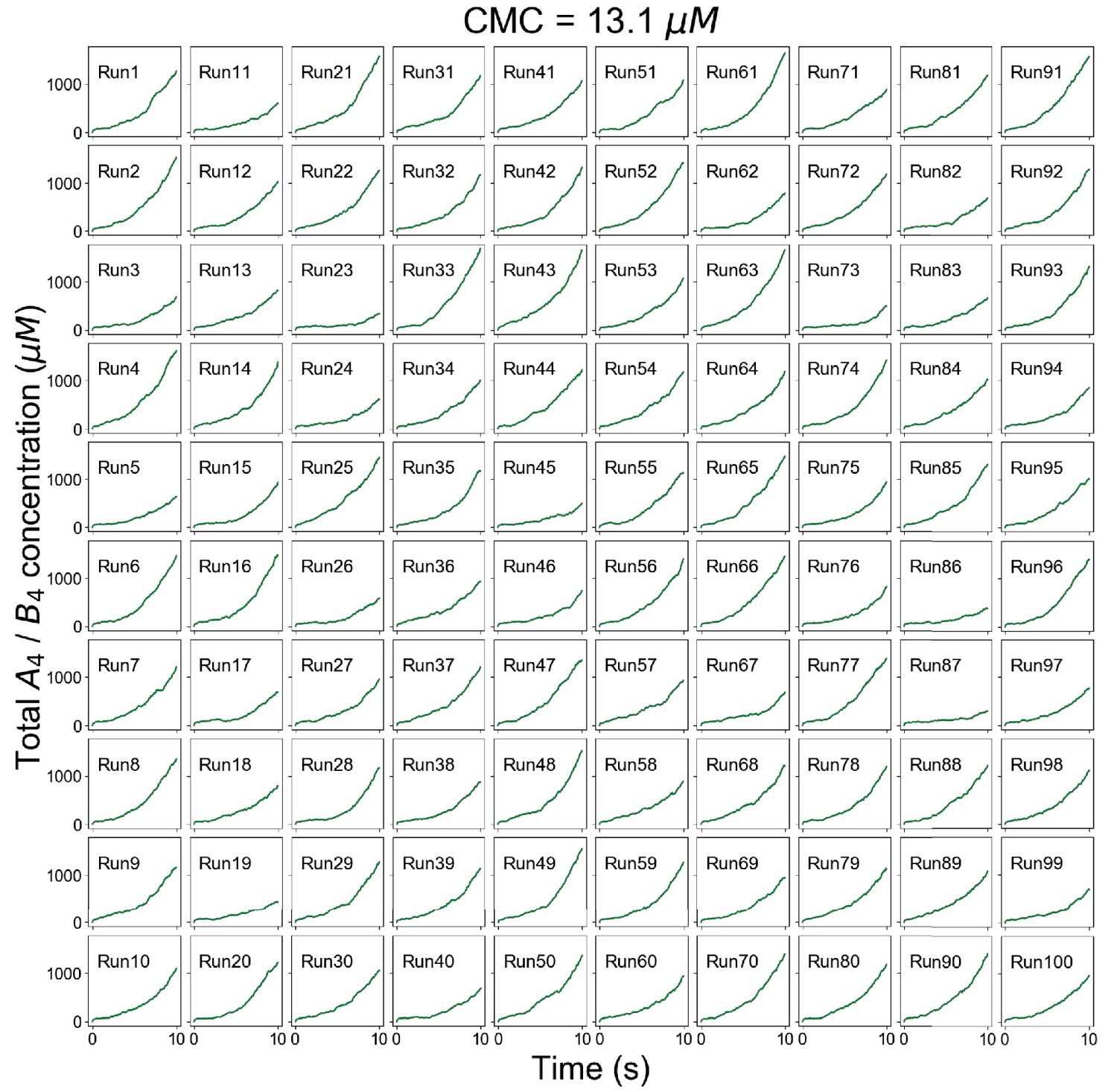
Individual trajectories of total molecular concentrations (A4 in magenta and B4 in green) at clamped monomer concentration (CMC) = 13.1 µM.
Figure 2—figure supplement 4
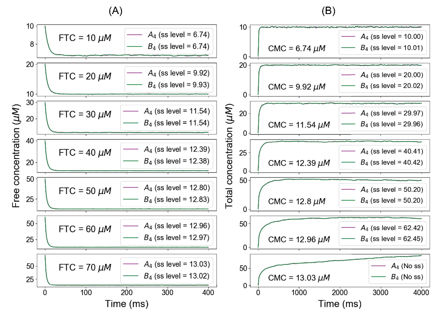
Summary of fixed total concentration (FTC) and clamped monomer concentration (CMC) method predictions.
Below the phase boundary, if we clamp the free concentrations from the FTC approach (A), we recover the identical total concentrations at steady state in CMC approach (B). Above the concentration threshold (example of FTC = 70 µM), clamping the free concentrations from FTC method no longer yields the same steady-state level (CMC = 13.01 µM).
Figure 3 with 1 supplement

The Ksp defines a threshold for unlimited growth of clusters even when the individual concentrations of heterotypic multivalent binding partners are unequal.
-
Figure 3—source data 1
Source data for Figure 3.
- https://cdn.elifesciences.org/articles/67176/elife-67176-fig3-data1-v2.xlsx
Figure 3—figure supplement 1
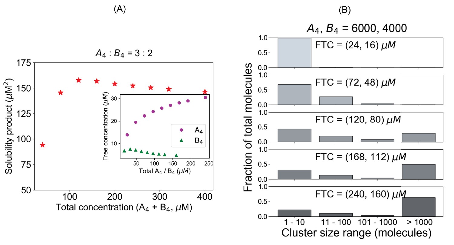
System (A4– B4) deviates from a fixed Ksp when initial conditions are not stoichiometrically matched.
(A) Solubility product profile and (B) cluster size distributions with unequal stoichiometric ratio. In all these simulations, we maintain a fixed number of 6000 A4 and 4000 B4 molecules and change the volume to alter the concentrations.
Figure 4
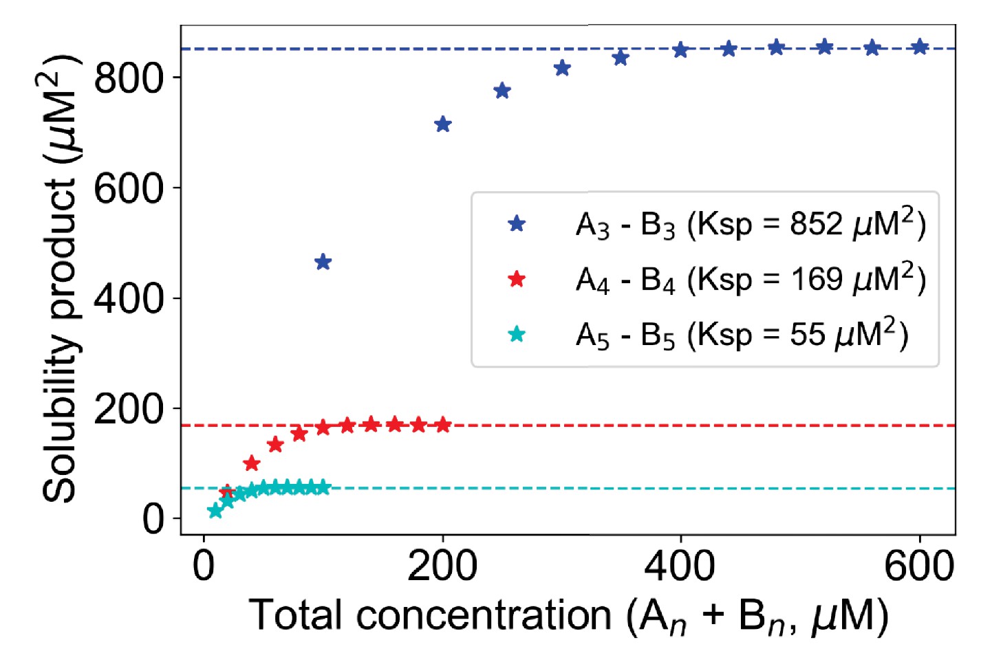
Change of Ksp with molecular valency.
For 3,3 case (blue stars), molecular counts of each type = [500, 1000, 1500, ..., 3000]. For 4,4 case (red stars), molecular counts of each type = [100, 200, 300, ..., 1000]. For 5,5 case (cyan stars), molecular counts of each type = [50, 100, 150, ..., 500]. Kd is set to 3500 molecules in all these cases. Horizontal dashed lines indicate the Ksp of the corresponding system.
-
Figure 4—source data 1
Source data for Figure 4.
- https://cdn.elifesciences.org/articles/67176/elife-67176-fig4-data1-v2.xlsx
Figure 5 with 1 supplement
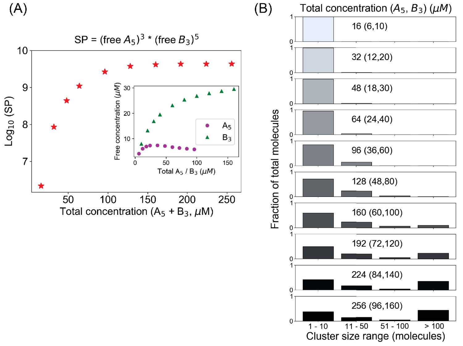
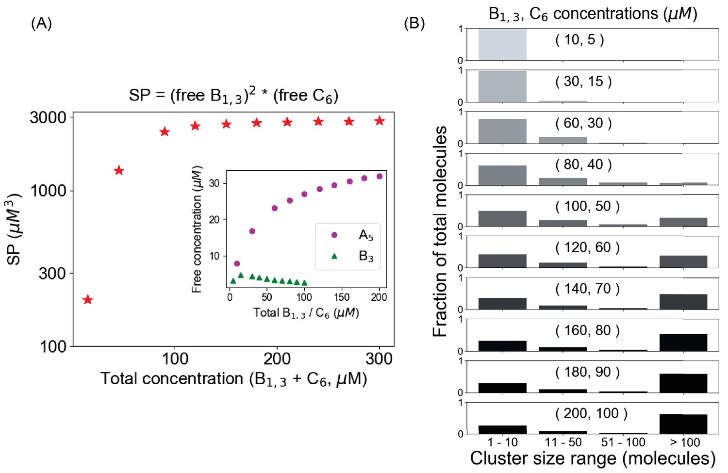
A mixed-valent binary system obeys a stoichiometry-adjusted Ksp.
(A) Logarithm of solubility product (SP) as a function of total concentrations (A5 + B3). Inset shows the variation of free molecular concentrations w.r.t. their initial total concentrations. Molecules are added at a fixed volume to vary the total concentrations. (B) Cluster size distributions become more bimodal as we go beyond the critical concentration (128 µM in this case).
-
Figure 5—source data 1
Source data for Figure 5.
- https://cdn.elifesciences.org/articles/67176/elife-67176-fig5-data1-v2.xlsx
Figure 5—figure supplement 1

Simple product of free molecular concentrations does not work for mixed-valent binary systems.
Here, solubility product = Free A5 * Free B3.
Figure 6 with 3 supplements

Titration of one molecular component in a heterotypic condensate yields correlations with the experimental results [Riback et al., 2020].
We begin with 120 µM B1,3 and 60 µM C6, which displays a bimodal cluster distribution (condensate formation; Supp. Fig. S6); we then titrate up A3 concentration from 1 µM to 200 µM. (A–C) Free A3 (monomeric) concentration, bound A3 (total A3 – free A3) concentration and their ratio as a function of total A3 concentrations. Inset figures are replotted from the data reported in Riback et al., 2020. To guide the eye, we fit their experimental data to a generic function, y = a * xn where a and n are pre-exponent and exponent factors, respectively. The red lines in the inset plots demonstrate the 'expected' trend if the condensation is purely driven by homotypic interactions. (D) Blue triangles correspond to the solubility product (SP) of the three-component system when A3 is being titrated up gradually, with fixed total [B1,3] = 120 µM and [C6] = 60 µM. Red stars indicate the scenario when we simultaneously change concentrations of all three components, keeping a concentration ratio of 2:6:3.
-
Figure 6—source data 1
Source data for Figure 6.
- https://cdn.elifesciences.org/articles/67176/elife-67176-fig6-data1-v2.xlsx
Figure 6—figure supplement 1
A pair of trivalent (B1,3) and hexavalent (C6) molecules forms condensates when their solubility product reaches to a plateau.
(A) Change of solubility product (SP) as a function of total concentration; Ksp ~ 2700 µM3 for this binary system. Inset shows the change of individual components. (B) Cluster size distributions as a function of total concentration. The distribution starts to become bimodal beyond 120 µM (80 µM B1,3, 40 µM C6), which is the threshold concentration when SP converges to the Ksp.
Figure 6—figure supplement 2
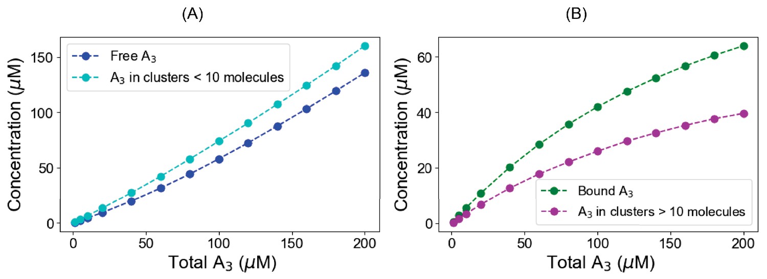
Titration profiles for A3 in ternary system.
In a pre-formed condensate (120 µM B1,3 + 60 µM C6), we gradually titrate up the A3 and calculate concentrations both in the free and clustered state. (A) Blue points represent the free (monomeric) A3 concentrations where cyan points correspond to the total A3 present in clusters, which is less than 10 molecules in size. (B) Green points represent the bound A3 (total A3 – free A3) concentrations while magenta points indicate total A3 present in the clusters greater than 10 molecules.
Figure 6—figure supplement 3
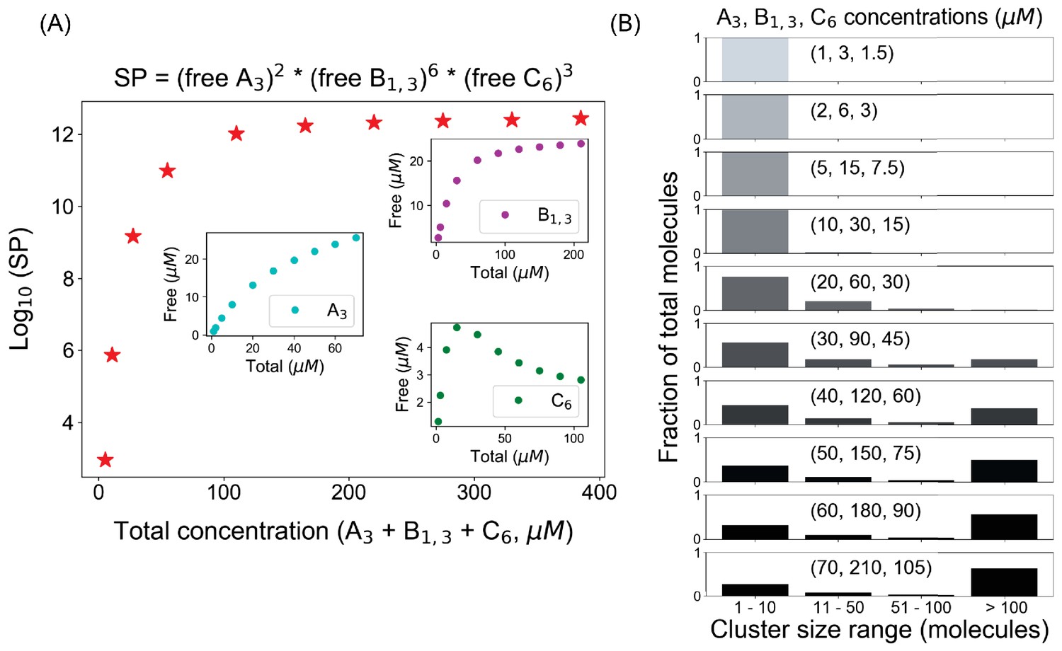
Solubility product(SP) profile for A3–B1,3–C6 system.
(A) With a fixed number of molecules (A3 = 200, B1,3 = 600, C6 = 300 molecules), we change the volume of the system to alter the molecular concentrations. Inset plots show the concentration changes of individual components. (B) Cluster size distributions at different total concentrations, which starts to become bimodal after 165 µM (30, 90, 45 µM) marked by the Ksp (sixth point in SP plot).
Figure 7 with 7 supplements
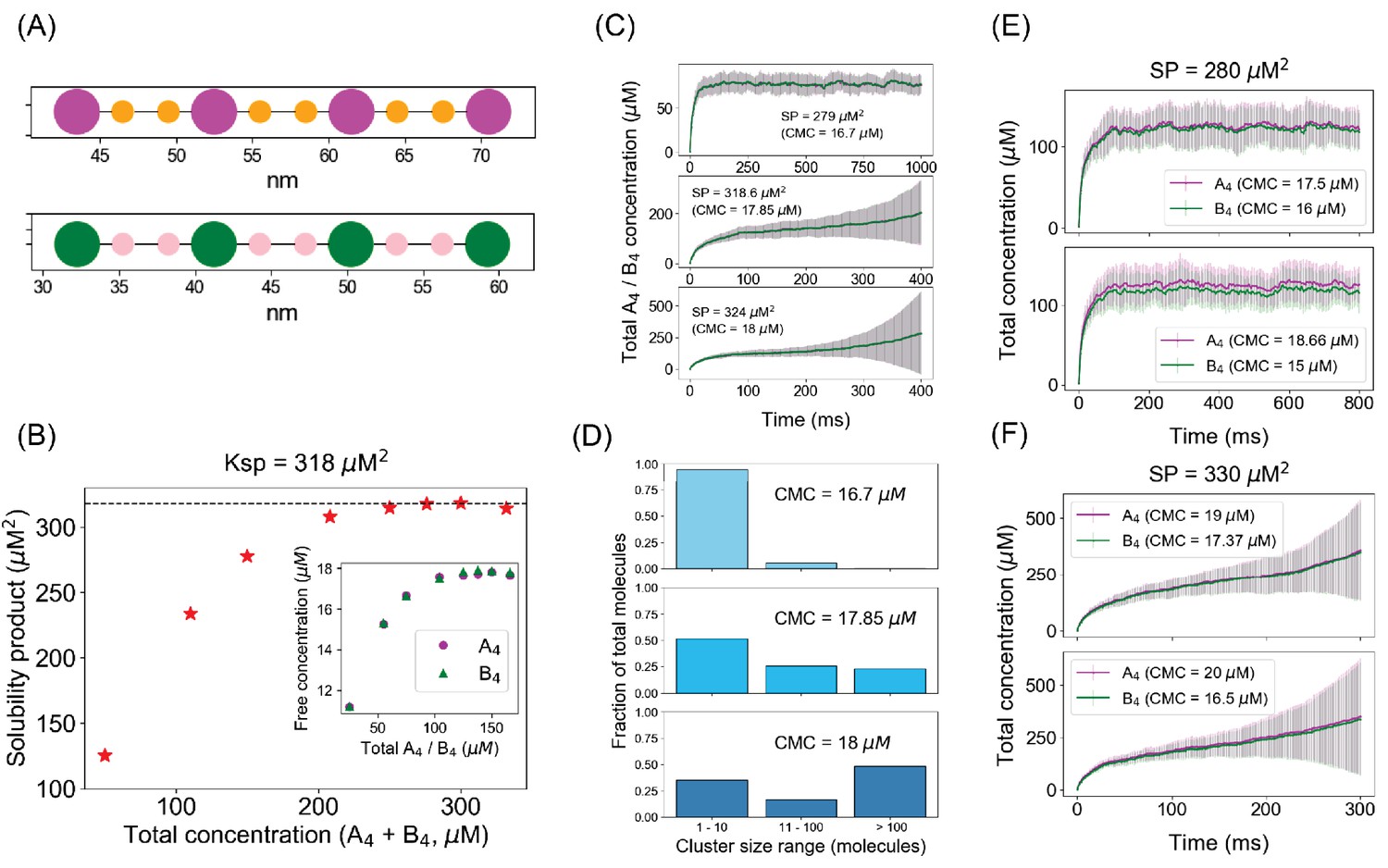
Spatial simulations demonstrate similar phase boundary behavior as network-free simulator (NFsim).
(A) SpringSaLaD representations of a pair of tetravalent binders. A4a and B4b consist of four magenta and green spherical binding sites (radius = 1.5 nm) and six orange and pink linker sites (radius = 0.75 nm). Diffusion constants for all the sites are set to 2 µm2/s. For individual binding, dissociation constant, Kd = 350 µM (Kon = 20 µM−1.s−1, Koff = 7000 s−1). Simulation time constants, dt (step size) = 10−8 s−1 , dt_spring (spring relaxation constant) = 10−9 s−1 . (B) Solubility product (SP) profile of the spatial system. We place a total of 200 molecules (100 A4a + 100 B4b) in 3D boxes with varying volumes and quantify the monomer concentrations (free A4a and free B4b) at steady states. Each data point is an average over 100 trajectories. Solubility product constant (Ksp) = 318 µM2, the horizontal dashed line. (C) Total molecular concentration profiles for three clamped monomer concentrations (CMCs). The solid lines and error bars represent the mean and standard deviation over 50 trajectories. (D) Cluster size distributions at the last time point of CMC trajectories, that is, 1000 ms for CMC = 16.7 µM, 400 ms for CMC = 17.85 µM and 18 µM. More detailed histograms without binning are shown in Figure 7—figure supplement 1. (E, F) Irrespective of individual monomer concentrations, total molecular concentrations converge to steady states as long as the solubility product (SP = 280 µM2) < Ksp (E) and diverge with time when SP (= 330 µM2) > Ksp (F). The solid lines and error bars represent the mean and standard deviation over 50 trajectories.
-
Figure 7—source data 1
Source data for Figure 7.
- https://cdn.elifesciences.org/articles/67176/elife-67176-fig7-data1-v2.xlsx
Figure 7—figure supplement 1
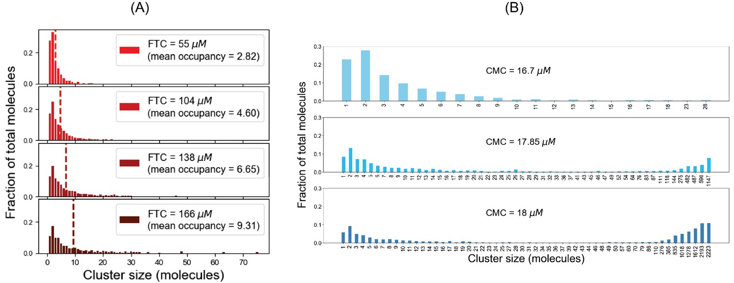
For SpringSaLaD system, (A) cluster size distributions at steady state (sampled from last time point) for different fixed total concentrations; (B) cluster size distributions at last time point for different clamped monomer concentrations.
Figure 7—figure supplement 2
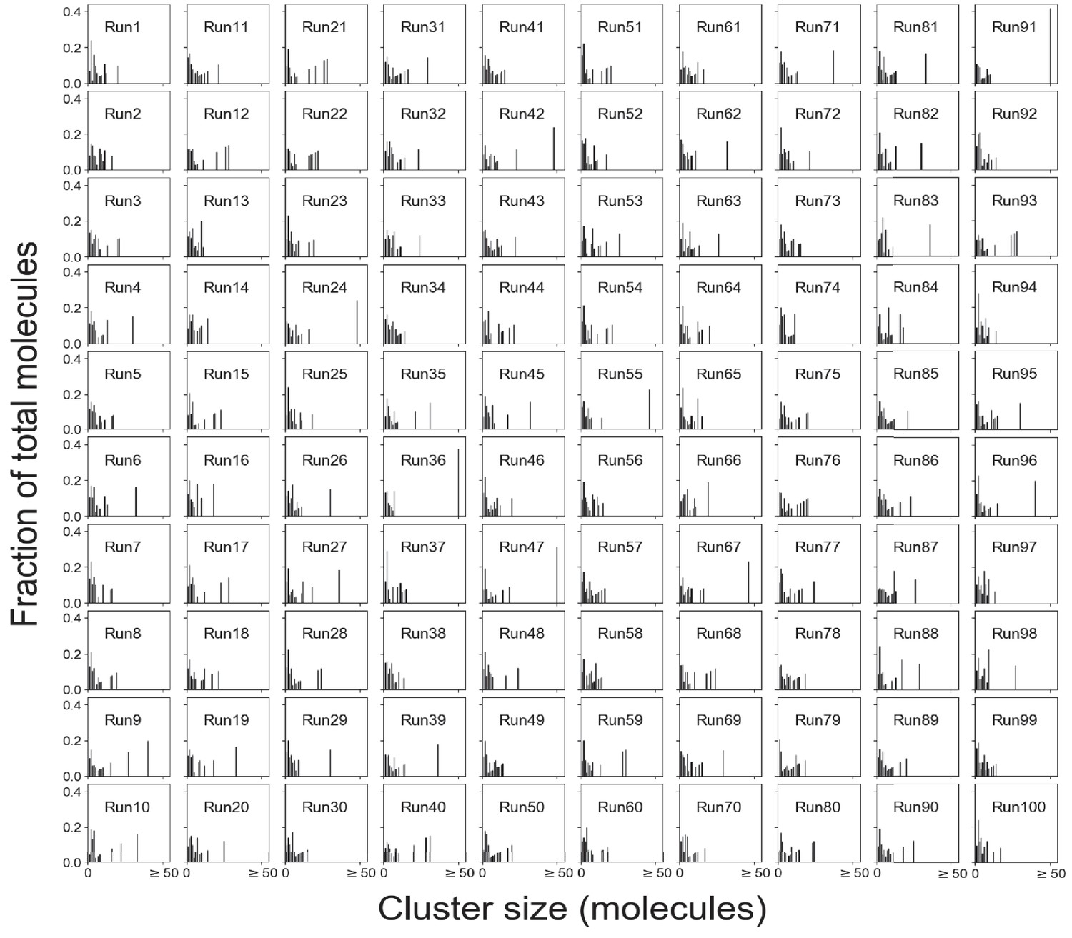
Cluster size distributions for single SpringSaLaD trajectories.
Total molecules = 200 (100 A4a and 100 B4b). Molecular concentrations = 332 µM, which is above the phase transition threshold (~276 µM). Clusters containing more than 50 molecules are shown with a single bar.
Figure 7—figure supplement 3
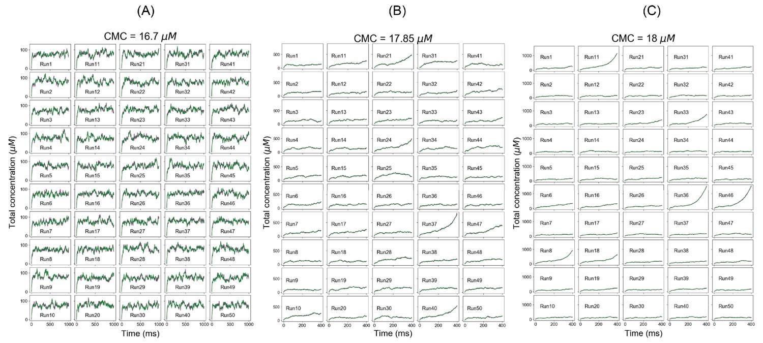
For SpringSaLaD system, individual total concentration trajectories at (A) clamped monomer concentration (CMC) = 16.7 µM (below Ksp), (B) CMC = 17.85 µM (at Ksp), and (C) CMC = 18 µM (above Ksp).
Magenta and green traces correspond to total A4 and total B4 concentration, respectively.
Figure 7—video 1
Single trajectory for spatial simulations below Ksp.
It has three synchronous displays: (1) visualization of molecular diffusion and cluster formation (right panel); (2) total molecular concentrations (free + bound) at a given time point (lower-left panel); and (3) distribution of molecular clusters at a given time point (upper-left panel).
Figure 7—video 2
Single trajectory for spatial simulations at Ksp.
It has three synchronous displays: (1) visualization of molecular diffusion and cluster formation (right panel); (2) total molecular concentrations (free + bound) at a given time point (lower-left panel); and (3) distribution of molecular clusters at a given time point (upper-left panel).
Figure 7—video 3
Single trajectory for spatial simulations slightly above Ksp.
It has three synchronous displays: (1) visualization of molecular diffusion and cluster formation (right panel); (2) total molecular concentrations (free + bound) at a given time point (lower-left panel); and (3) distribution of molecular clusters at a given time point (upper-left panel).
Figure 7—video 4
Dynamics of individual clusters below (left panel) and above (right panel) the Ksp.
The left panel was generated from the same data as Figure 7—video 1; the right panel was generated from the same data as Figure 7—video 3. We track the centroid of individual clusters and compute a radius of gyration around that center. The radius of gyration is scaled down by a factor of 4 to aid visualization of individual clusters.
Additional files
Download links
A two-part list of links to download the article, or parts of the article, in various formats.
Downloads (link to download the article as PDF)
Open citations (links to open the citations from this article in various online reference manager services)
Cite this article (links to download the citations from this article in formats compatible with various reference manager tools)
The solubility product extends the buffering concept to heterotypic biomolecular condensates
eLife 10:e67176.
https://doi.org/10.7554/eLife.67176


