Rotational dynamics in motor cortex are consistent with a feedback controller
- The BioRobotics Institute, Scuola Superiore Sant'Anna, Italy
- Centre for Neuroscience Studies, Queen's University, Canada
- Centre for Computation, Mathematics and Physics, University College London, United Kingdom
- Department of Physiology, University of California, San Francisco, United States
Figures
Figure 1
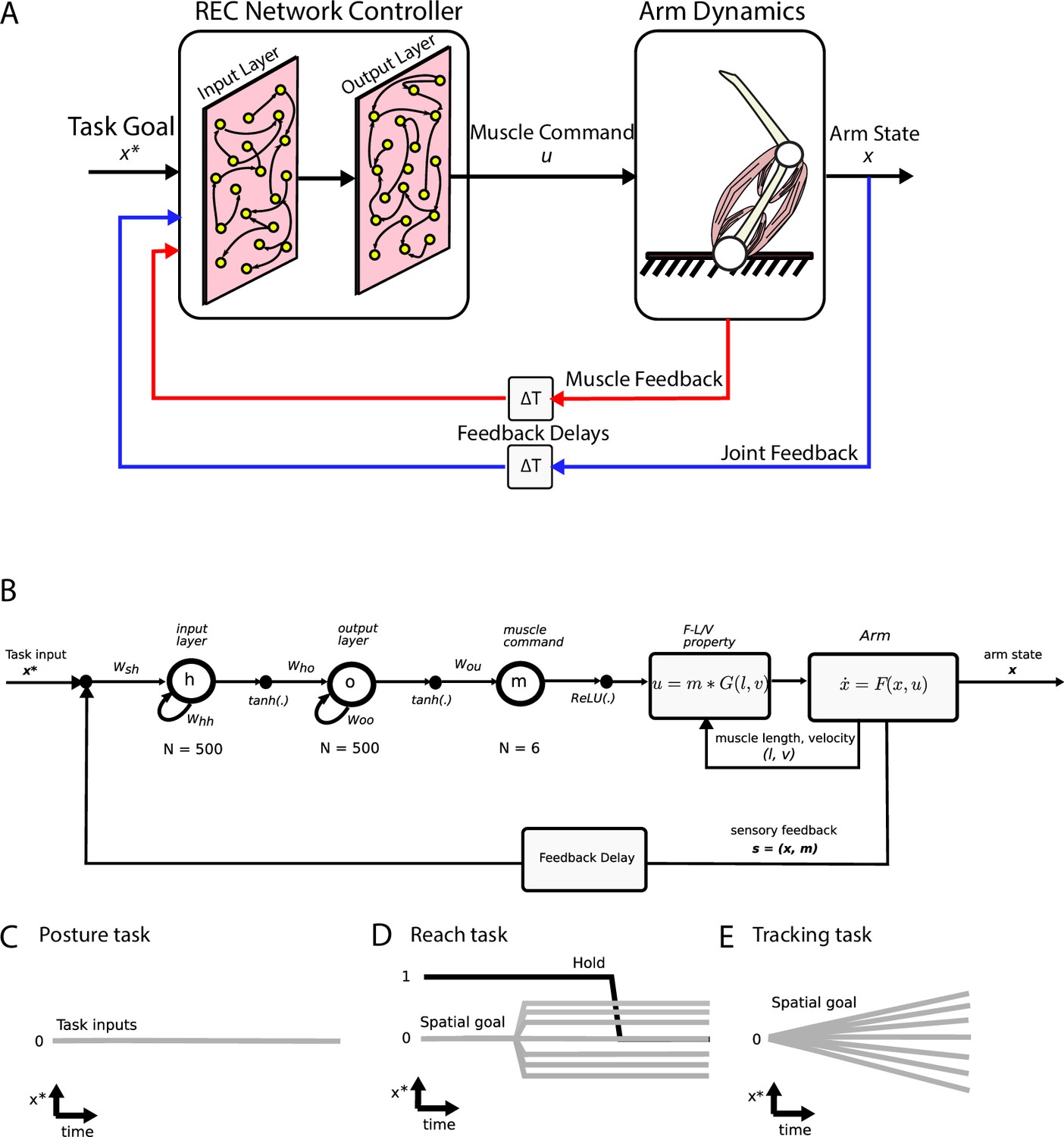
Simulation setup.
(A) Schematic of the two-link model of the arm and the neural network. The arm had two joints mimicking the shoulder and elbow (arm dynamics: joints are white circles) and was actuated using six muscles (pink banded structures). Muscle activity was generated by the neural network (muscle command). The network was composed of two layers (input and output layers) with recurrent connections between units within each layer. The network received delayed (ΔT) sensory feedback from the limb in the form of joint angles and velocities (joint feedback, blue line), and muscle activities (muscle feedback, red line). Delays were set to 50 ms to match physiological delays. The network also received input about the desired location of the limb (task goal). (B) Computational graph for the same network depicted in (A). Whh and Woo are the recurrent connections for the input and output layers, respectively. For the NO-REC network, these connections were set to zero and remained at zero when optimizing. Wsh are the connection weights between the inputs to the input layer and Who are the connection weights between the input layer and the output layer. Tanh activation functions were used for the network layers and a rectified linear unit (ReLU) was used for the muscle layer. Muscle activity (m) was then converted to joint torques (u) while taking into account force-length (F-L) and force-velocity (F-V) properties of muscles. Joint torques were used to update the arm state (x) and sensory feedback (s) about the arm state and muscle activities was fed back into the input layer following a feedback delay. (C–E) Visual depictions of the task inputs to the network (x*) for each of the behaviours. There was no task input for the posture task (C). For the reach task (D), the task input reflected the spatial end position of the target as well as a GO cue (hold command, thick black line). For the tracking task (E), the task input reflected the spatial position of the moving target at each time point.
Figure 2
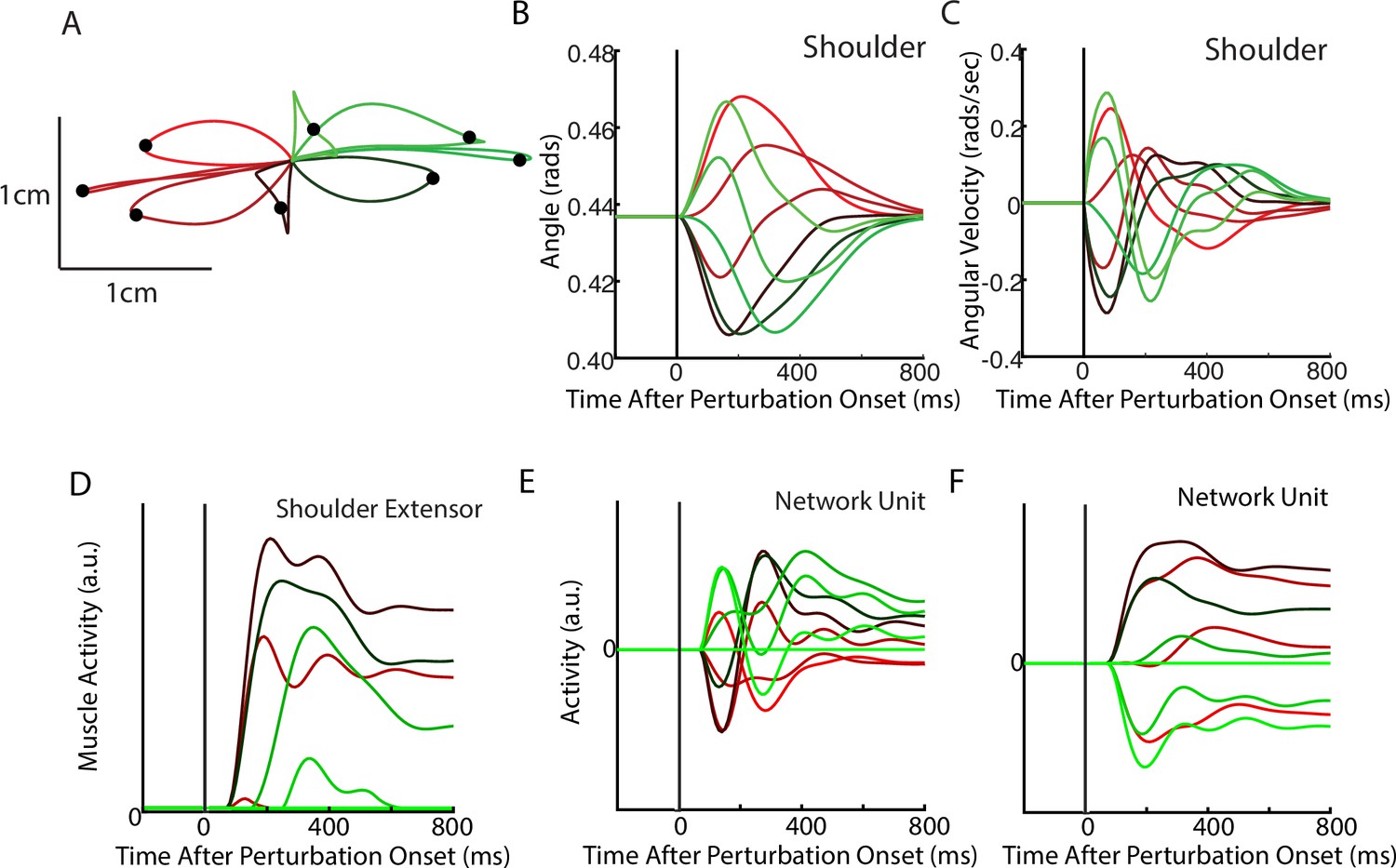
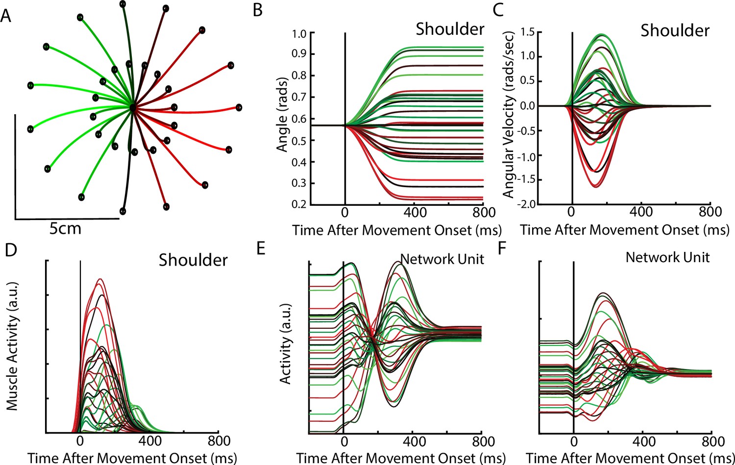
Posture perturbation task performed by neural network.
(A) Hand paths when mechanical loads were applied to the model’s arm. Due to the anisotropy in the biomechanics, the trajectories across the different loads are asymmetric. Black dots denote the hand’s location 300 ms after the load onset. (B, C) Shoulder angle and angular velocity aligned to the load onset. (D) Activity of the shoulder extensor aligned to load onset. (E, F) The activities of two example units from the output layer of the network. The colors in (A–F) correspond to different directions of load.
Figure 3 with 2 supplements
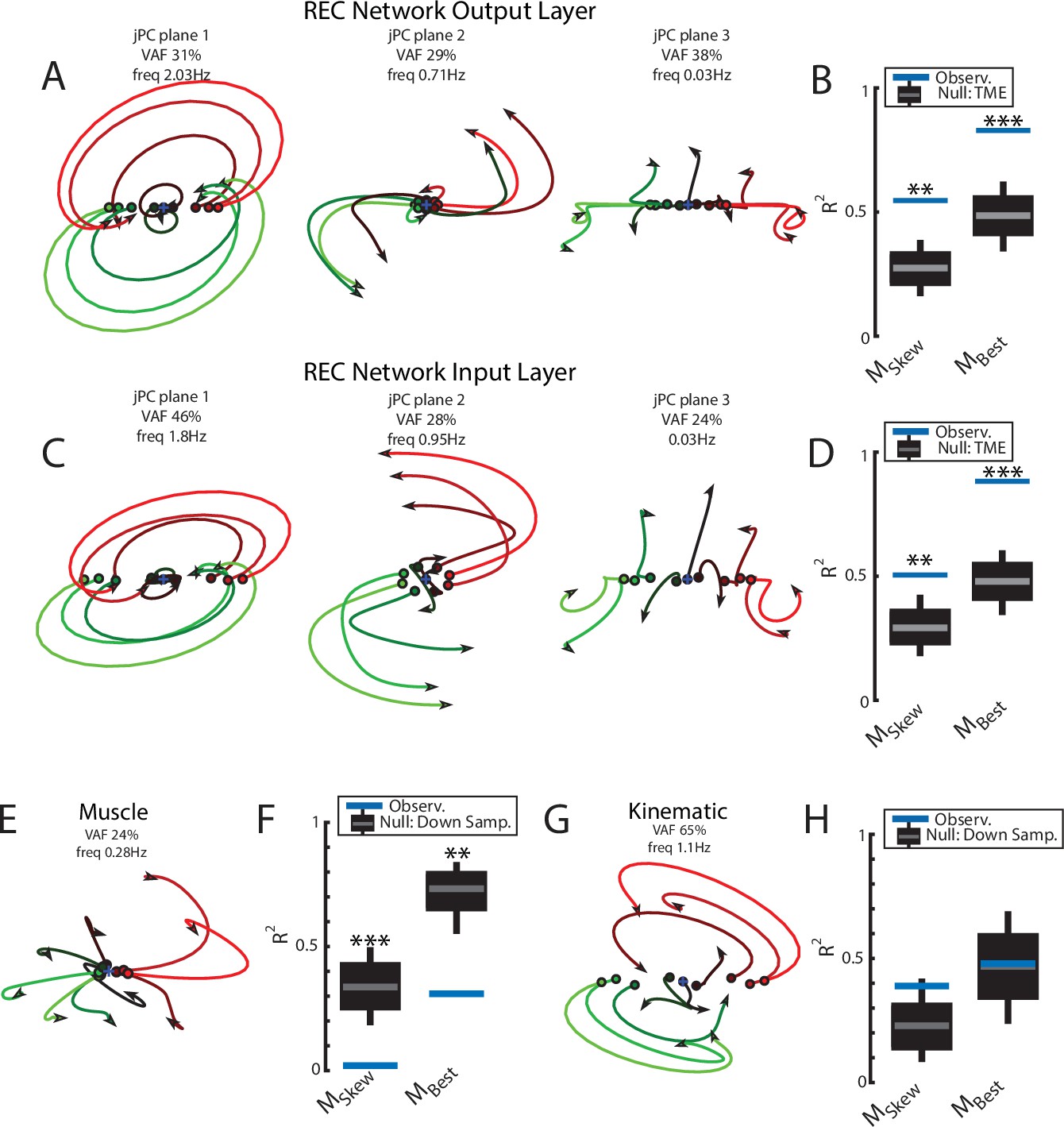
Population dynamics of the network during posture.
(A) The top3 jPC planes from the activity in the output layer of the network. Dynamics were computed from 70 ms to 370 ms after the load onset. Different colors denote different load directions. (B) The goodness of fit (black horizontal line) of the network activity to the constrained (MSkew left) and unconstrained (MBest right) dynamical systems. Null distributions were computed using tensor maximum entropy (TME). Gray bars denote the median, the boxes denote the interquartile ranges, and the whiskers denote the 10th and 90th percentiles. (C, D) same as (A, B) except for the input layer of the network. (E, F) and (G, H) same as (A, B) except for the muscle activities and kinematic inputs into the network, respectively. Null distributions were computed from the down-sampled neural activity for (F) and (H). VAF, variance accounted for.
Figure 3—figure supplement 1
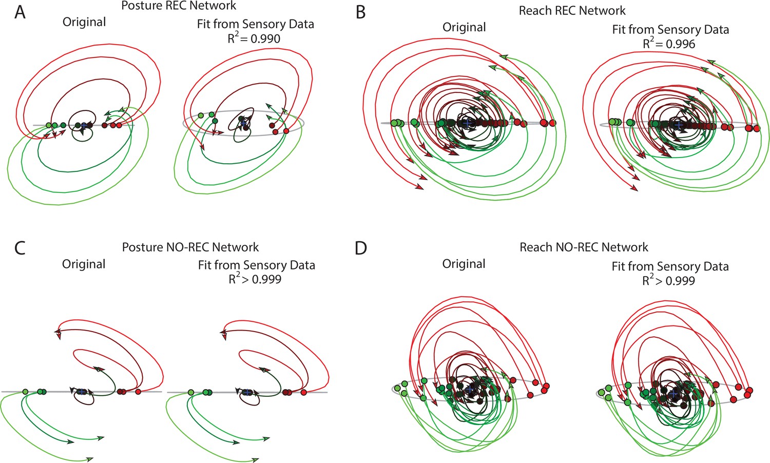
Decoding output layer trajectories using sensory input.
(A) The top jPC plane from the output layer activities (left) and the decoded activity using only sensory feedback (right) during the perturbation posture task. R2 reflects the fit quality across all six jPC planes. (B) same as (A) for the center-out reaching task. (C, D) same as (A, B) except for the NO-REC networks.
Figure 3—figure supplement 2
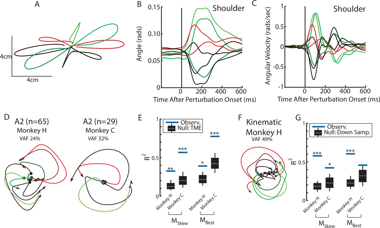
Population dynamics in somatosensory cortex during posture task from Chowdhury et al., 2020.
(A) Hand paths for Monkey H using an endpoint manipulandum where loads were applied that displaced the hand from the starting position. (B, C) The shoulder flexion angle and angular velocity across the load directions. (D) The top jPC plane from activity recorded in somatosensory area 2. (E) Goodness of fits to the constrained (MSkew left) and unconstrained (MBest right) dynamical systems. Null distributions were computed using tensor maximum entropy. (F, G) same as (D, E) except for the kinematic signals. Null distributions were computed from the down-sampled neural activity. Data from Chowdhury et al., 2020. *p<0.05, **p<0.01, ***p<0.001.
Figure 4
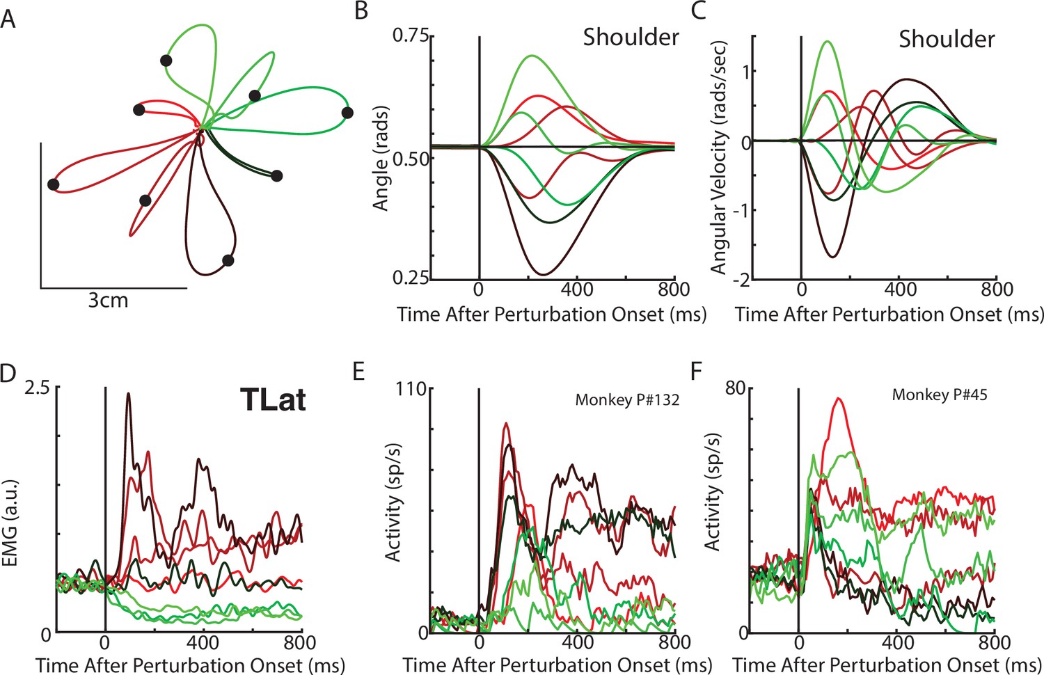
Posture perturbation task performed by monkeys.
(A) Hand paths for Monkey P when mechanical loads were applied to its arm. (B, C) Shoulder angle and angular velocity aligned to the onset of the mechanical loads. (D) Recording from the lateral head of the triceps (elbow extensor) during the posture perturbation task. (E, F) Example neurons from motor cortex aligned to perturbation onset.
Figure 5 with 3 supplements
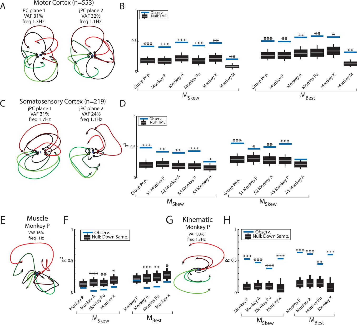
Population dynamics across motor and somatosensory cortex.
(A) The top-2 jPC planes from activity recorded in motor cortex (MC) pooled across all monkeys. (B) Goodness of fits to the constrained (MSkew left) and unconstrained (MBest right) dynamical systems for MC activity for the pooled activity across monkeys (Group Pop.) and for each individual monkey. Null distributions were computed using tensor maximum entropy (TME). (C, D) same as (A, B) for somatosensory recordings. (E) The top jPC plane from muscle activity from Monkey P. (F) Goodness of fits to the muscle activity for the constrained and unconstrained dynamical systems for each monkey. (G, H) same as (E, F) for kinematic signals. (B, D, F, H) Gray bars denote the medians, the boxes denote the interquartile ranges, and the whiskers denote the 10th and 90th percentiles. *p<0.05, **p<0.01, ***p<0.001.
Figure 5—figure supplement 1
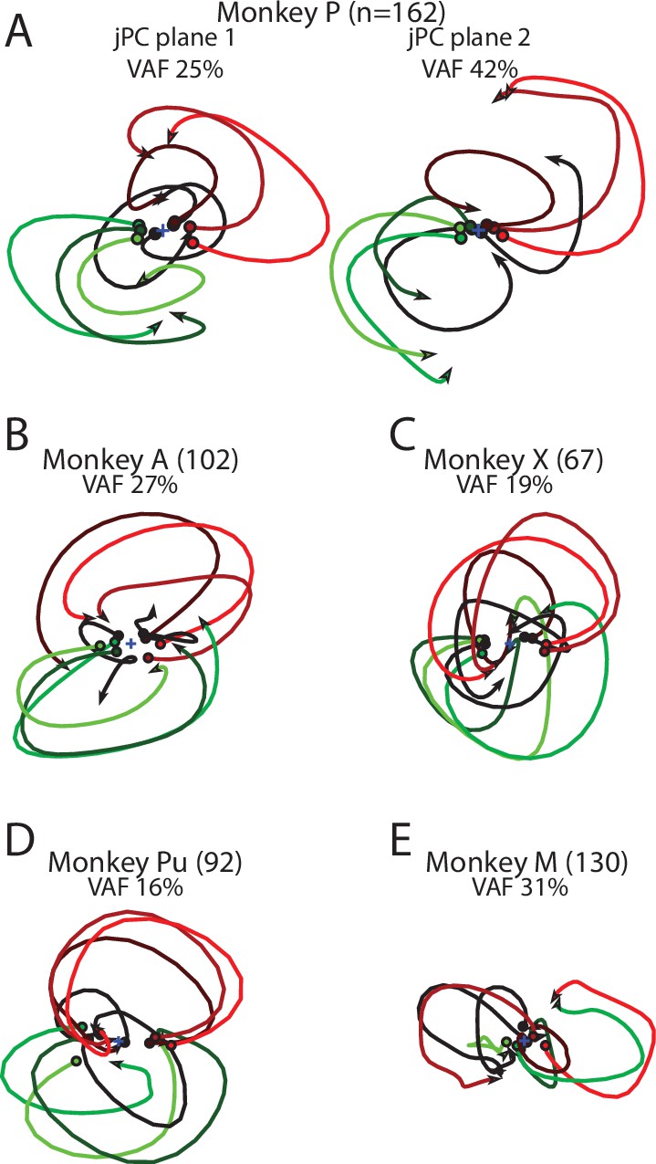
Population dynamics in motor cortex (MC) for individual monkeys.
(A) The top-2 jPC planes from activity recorded in MC in Monkey P. (B) The top jPC plane from activity recorded in MC in Monkey A. (C–E) same as (B) for Monkeys X, Pu, and M.
Figure 5—figure supplement 2
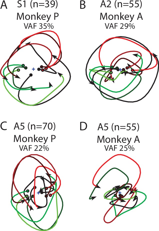
Population dynamics in somatosensory cortex for individual monkeys.
Data are presented the same as Figure 5—figure supplement 1 for S1 in Monkey P (A), A2 in Monkey A (B), A5 in Monkey P (C), and A5 in Monkey A (D).
Figure 5—figure supplement 3
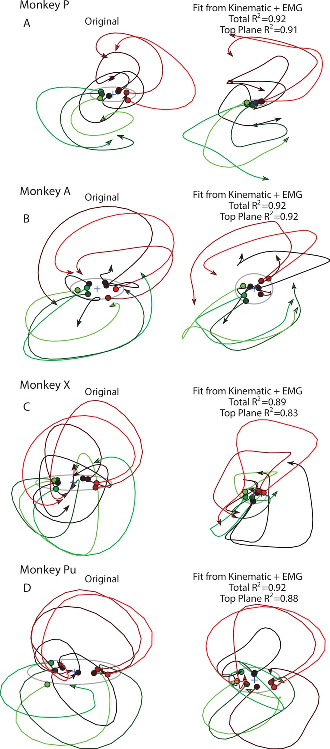
Decoding M1 activity using kinematic and muscle activities.
Data presented the same as in Figure Supplementary 1 except for individual monkeys.
Figure 6 with 2 supplements
Delayed reach task by the network.
(A) The hand paths by the model’s arm from the starting position (center) to the different goal locations (black dots). Goals were placed 2 cm and 5 cm from the center location. (B, C) Shoulder angle and angular velocity aligned to movement onset. (D) Activity of the shoulder extensor aligned to GO cue onset. (E, F) The activities of two example units from the output layer of the network.
Figure 6—figure supplement 1
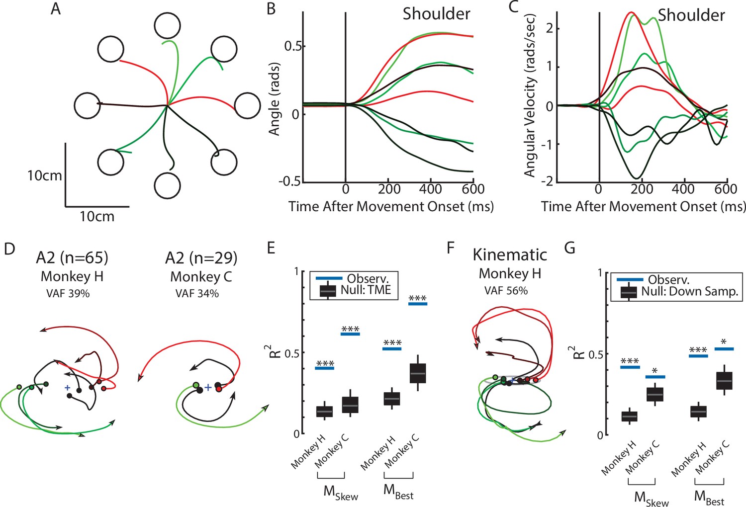
Population dynamics in somatosensory cortex during reaching from Chowdhury et al., 2020.
(A) Hand paths for Monkey H using an endpoint manipulandum to reach to different targets located in a center-out pattern. Targets were placed 12 cm from the starting position. (B, C) The shoulder flexion angle and angular velocity across the different reach directions (shoulder flexion angle defined in Chan and Moran, 2006). (D) The top jPC plane from activity recorded in somatosensory area 2. (E) Goodness of fits to the constrained (MSkew left) and unconstrained (MBest right) dynamical systems. Null distributions were computed using tensor maximum entropy (TME). (F–G) same as (D–E) except for the kinematic signals. Null distributions were computed from the down-sampled neural activity. *p<0.05, ***p<0.001.
Figure 6—figure supplement 2
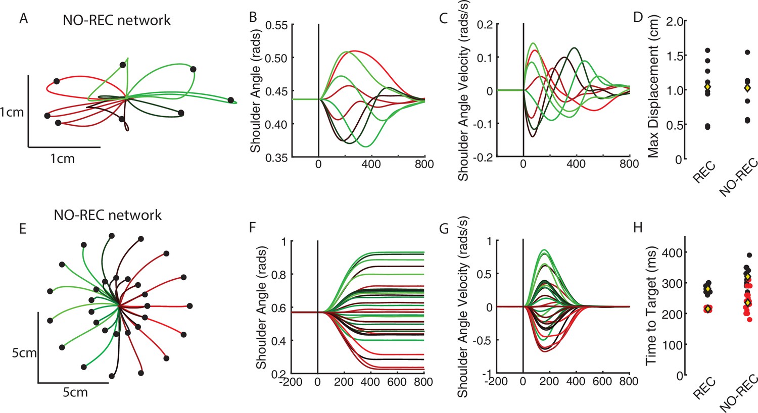
Behavioral performance of the NO-REC network.
(A) Hand paths generated by the NO-REC network during the perturbation posture task. (B, C) The shoulder angle and angular velocity, respectively. (D) Comparison of the maximum displacement of the limb for the REC and NO-REC network. Each perturbation direction is represented by a black dot. Yellow diamond reflects the mean. (E–G) same as (A–C) for the reaching task. (H) The time required by the network to move the limb from the starting position to the goal for both the REC and NO-REC networks. Red and black dots reflect the 2 cm and 5 cm reaches, respectively.
Figure 7
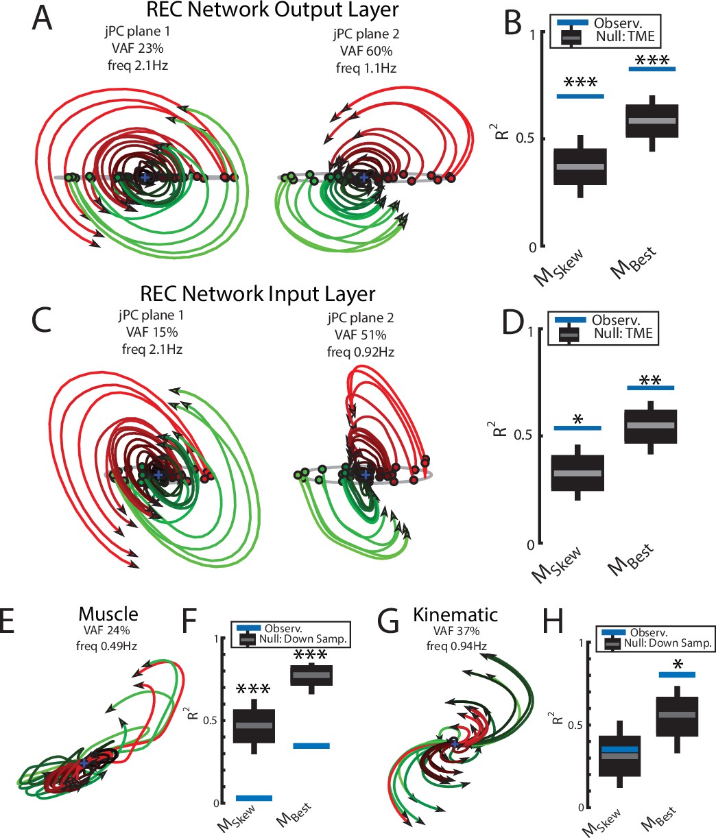
Population dynamics of the network during reaching.
(A) The top-2 jPC planes from the output layer of the network during reaching. (B) Goodness of fits for the network activity to the constrained (MSkew left) and unconstrained (MBest right) dynamical systems. Null distributions were computed using tensor maximum entropy (TME). (C, D) same as (A, B) for the input layer of the network. (E, F) and (G, H) same as (A, B) except for the muscle activities and kinematic inputs into the network, respectively. Null distributions were computed from the down-sampled neural activity. (B, D, F, H) Gray bars denote the medians, the boxes denote the interquartile ranges, and the whiskers denote the 10th and 90th percentiles. *p<0.05, **p<0.01, ***p<0.001.
Figure 8 with 4 supplements
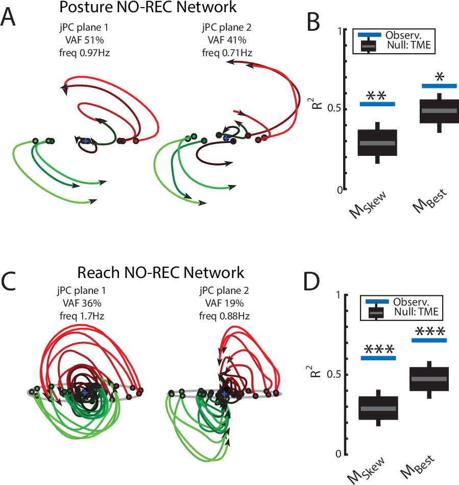
Population dynamics when trained without recurrent connections.
Networks were trained to perform the posture and reaching tasks without the recurrent connections within the MC and input layers. (A) The top-2 jPC planes from the output layer of the network during the posture task. (B) Goodness of fits for the network activity to the constrained (MSkew left) and unconstrained (MBest right) dynamical systems. Null distributions were computed using tensor maximum entropy (TME). (C, D) same as (A, B) for the output layer of the network during the reaching task. (C, D) Gray bars denote the medians, the boxes denote the interquartile ranges, and the whiskers denote the 10th and 90th percentiles. *p<0.05, **p<0.01.
Figure 8—figure supplement 1
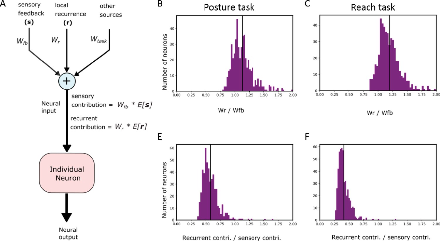
Analysis of REC network currents.
(A) Schematic showing the breakdown of the different current sources contributing to a neural unit’s output. Wfb, Wr, and Wtask refer to the synaptic weights onto the example neuron from the sensory feedback, neurons in the layer (local recurrence), and task goal inputs. (B, C) show the ratio of the local recurrent synaptic weights with the sensory synaptic weights across neurons for the posture and reaching task. (E, F) same as (B, C) for the currents generated by each source. Note currents are defined as the product of the activity of the source (E[∙]) and the synaptic weight (see (A)).
Figure 8—figure supplement 2
REC networks perform better with continuous sensory feedback when encountering novel motor noise.
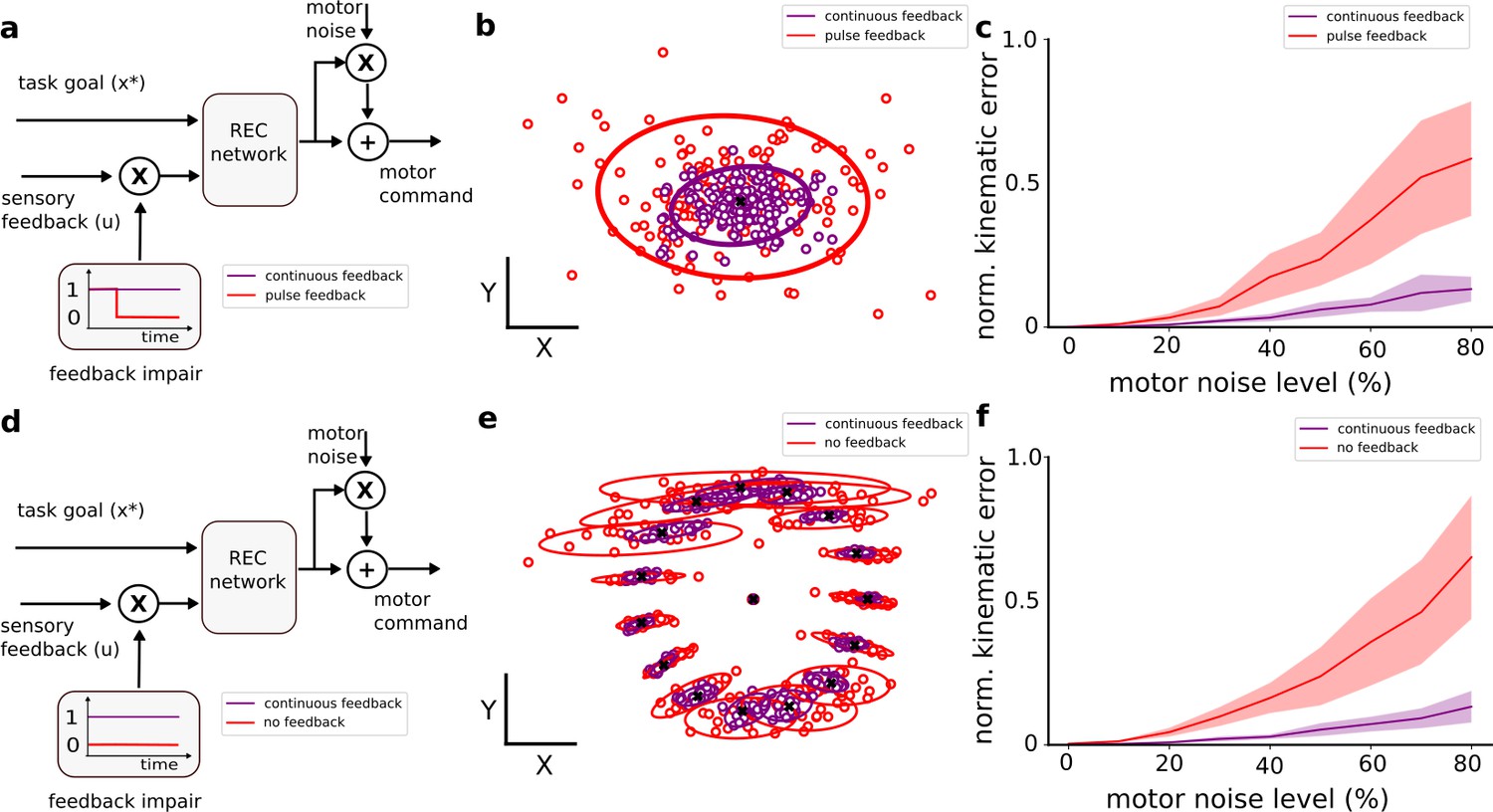
(A) Diagram showing the two network configurations during the perturbation posture task. One network received continuous sensory feedback whereas the other network only received sensory feedback for the first 200 ms (pulse feedback). Note the X symbol reflects the multiplication of the sensory feedback signal with the feedback impairment value. (B) The endpoint position of the limb for the two network configurations when 80% motor noise was added. Large circles denote the 95% confidence interval. (C) Increasing motor noise leads to greater impairment for the pulse-feedback network than the continuous feedback case. (D–F) Same as (A–C) for the reaching task. Note, the comparison was between networks with continuous feedback and networks with no sensory feedback during the task (no feedback).
Figure 8—figure supplement 3
Impact of sensory delays on rotational dynamics in network.
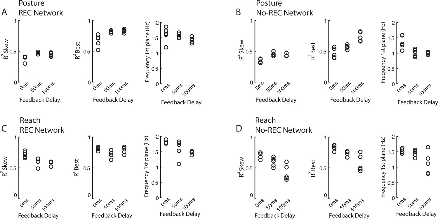
We simulated networks that received sensory feedback that had 0 ms, 50 ms, and 100 ms delays and each delay included five simulations from a random network initialization. (A) shows the dependence of fit quality and rotational frequency on sensory delays for the REC network during the perturbation posture task. (B) same as (A) for the NO-REC network. (C, D) same as (A, B) for the reaching task.
Figure 8—figure supplement 4
Cartesian-based sensory feedback reduces rotational dynamics.
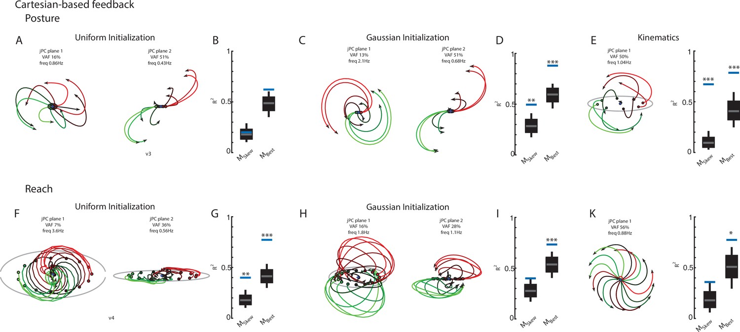
(A) The top-2 jPC planes for the REC network’s output layer. Networks received sensory feedback that reflected the hand position in a cartesian reference frame. (B) Fits for the constrained and unconstrained dynamical systems for the REC (left) and NO-REC (right) networks. (C) The top jPC plane for the hand kinematics in the cartesian reference frame. (D–F) same as (A–C) for the reaching task.
Figure 9
Networks trained on constant velocity tracking task exhibit dynamics that are less rotational.
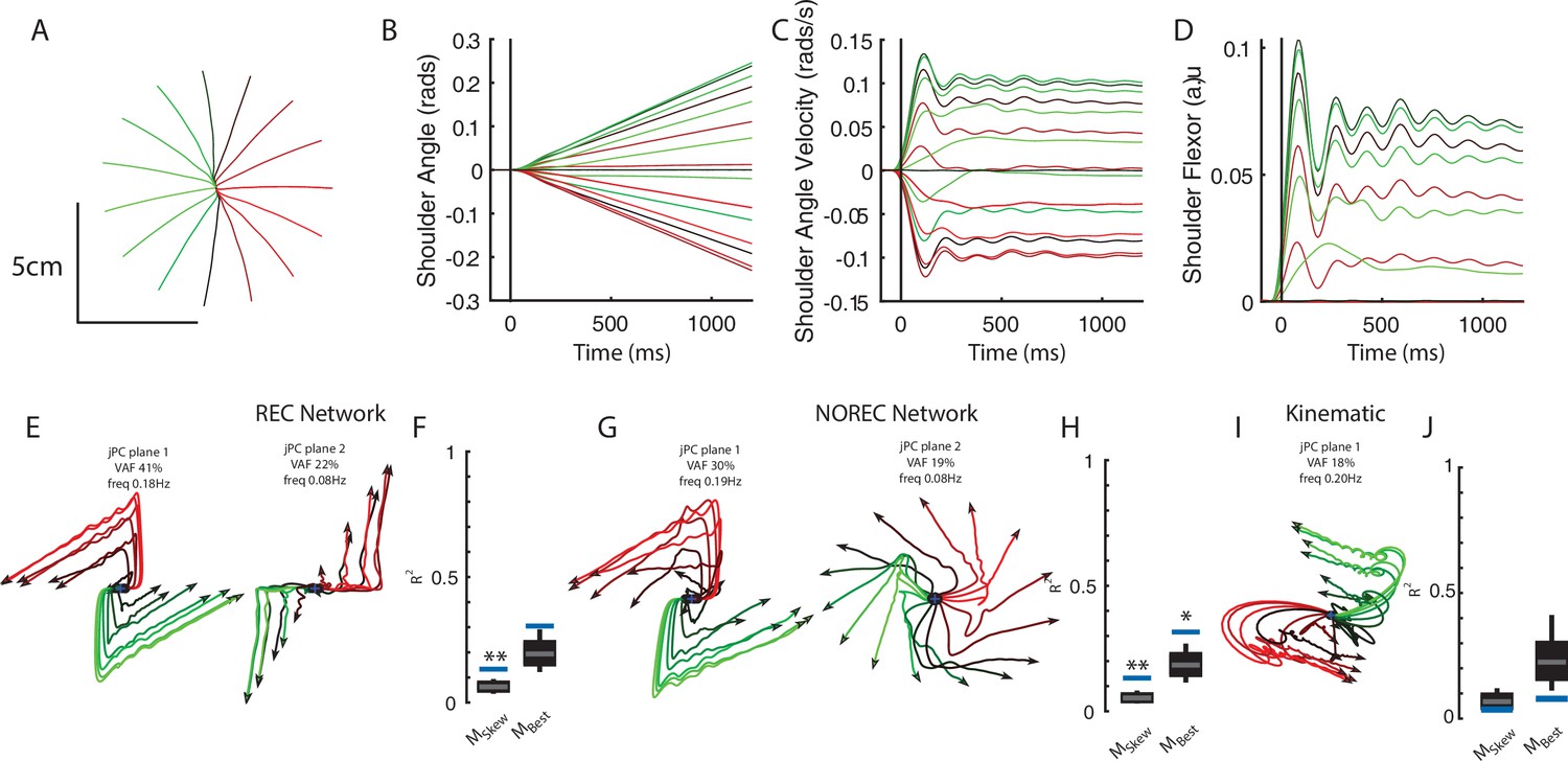
(A) Hand paths of the model performing the task. The limb started at the center and followed 1 of 16 trajectories in the radial direction. (B) and (C) Shoulder angle and angular velocity during the task. (D) Shoulder flexor muscle during task. (E) Activities for the output layer of the REC network for the top-2 jPC planes. Activity was examined from the start of movement till the end of the trial (~1.2 s). (F) Fits for the constrained and unconstrained dynamical systems. (G, H) same as (E, F) except for the NO-REC network. *p<0.05, **p<0.01.
Author response image 1

Additional files
Download links
A two-part list of links to download the article, or parts of the article, in various formats.
Downloads (link to download the article as PDF)
Open citations (links to open the citations from this article in various online reference manager services)
Cite this article (links to download the citations from this article in formats compatible with various reference manager tools)
Rotational dynamics in motor cortex are consistent with a feedback controller
eLife 10:e67256.
https://doi.org/10.7554/eLife.67256


