Figures and data in A simple regulatory architecture allows learning the statistical structure of a changing environment | eLife

Figures
Additional files

12 figures and 2 additional files

Figures

Figure 1

Download asset Open asset

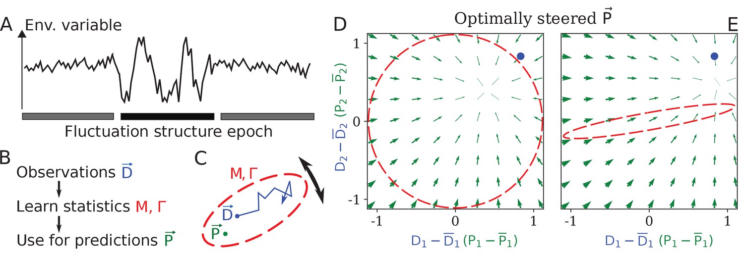
Learning environment statistics can benefit living systems, but is a difficult problem.

(A) An environment is characterized not only by its current state, but also by its fluctuation structure, such as variances and correlations of fluctuating environmental parameters. In this work, we consider an environment undergoing epochs that differ in their fluctuation structure. Epochs are long compared to the physiological timescale, but switch faster than the evolutionary timescale. (B) The fluctuation structure can inform the fitness-maximizing strategy, but cannot be sensed directly. Instead, it would need to be learned from past observations, and used to inform future behavior. (C) To formalize the problem, we consider a situation where some internal physiological quantities $\vec{P} (t)$ must track fluctuating external factors $\vec{D} (t)$ undergoing a random walk. Since it is impossible to react instantaneously, $\vec{P}$ always lags behind $\vec{D}$ . The dashed ellipse illustrates the fluctuation structure of $\vec{D}$ (encoded in parameters $M$ and Γ, see text), and changes on a slower timescale than the fluctuations of $\vec{D}$ . (D, E) The optimal behavior in the two-dimensional version of our problem, under a constrained maximal rate of change ${∥ \dot{P} ∥}^{2}$ . For a given current $\vec{D}$ (blue dot), the optimal control strategy would steer any current $\vec{P}$ (green arrows) toward the best guess of the future $\vec{D}$ , which depends on the fluctuation structure (red ellipse: (D) fluctuations are uncorrelated and isotropic; (E) fluctuations have a preferred direction). The optimal strategy is derived using control theory (Appendix 1, section 'Control theory calculation').

Figure 2

Download asset Open asset

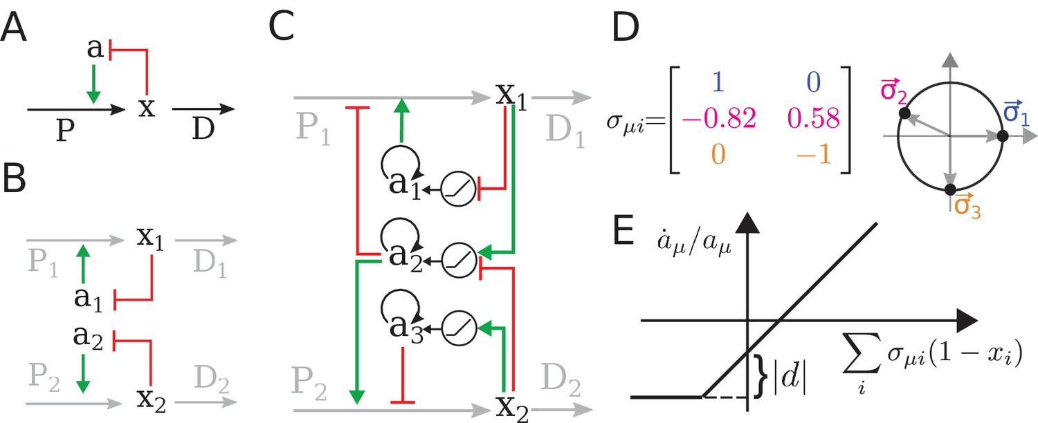
The regulatory architecture we consider is a simple generalization of end-product inhibition.

(A) Simple end-product inhibition (SEPI) for one metabolite. Green arrows show activation, red arrows inhibition. (B) Natural extension of SEPI to several metabolites. (C) We consider regulatory architectures with more regulators than metabolites, with added self-activation (circular arrows) and a nonlinear activation/repression of regulators $a_{μ}$ by the metabolite concentrations x_i (pictograms in circles). (D) Visualizing a regulation matrix $σ_{μ i}$ for two metabolites. In this example, the first regulator described by ${\vec{σ}}_{1}$ activates the production of x₁; the second inhibits x₁ and activates x₂. For simplicity, we choose vectors of unit length, which can be represented by a dot on the unit circle. This provides a convenient way to visualize a given regulatory architecture. (E) The nonlinear dependence of regulator activity dynamics ${\dot{a}}_{μ} / a_{μ}$ on metabolite concentrations x_i in our model (see Equation 4).

Figure 3

Download asset Open asset

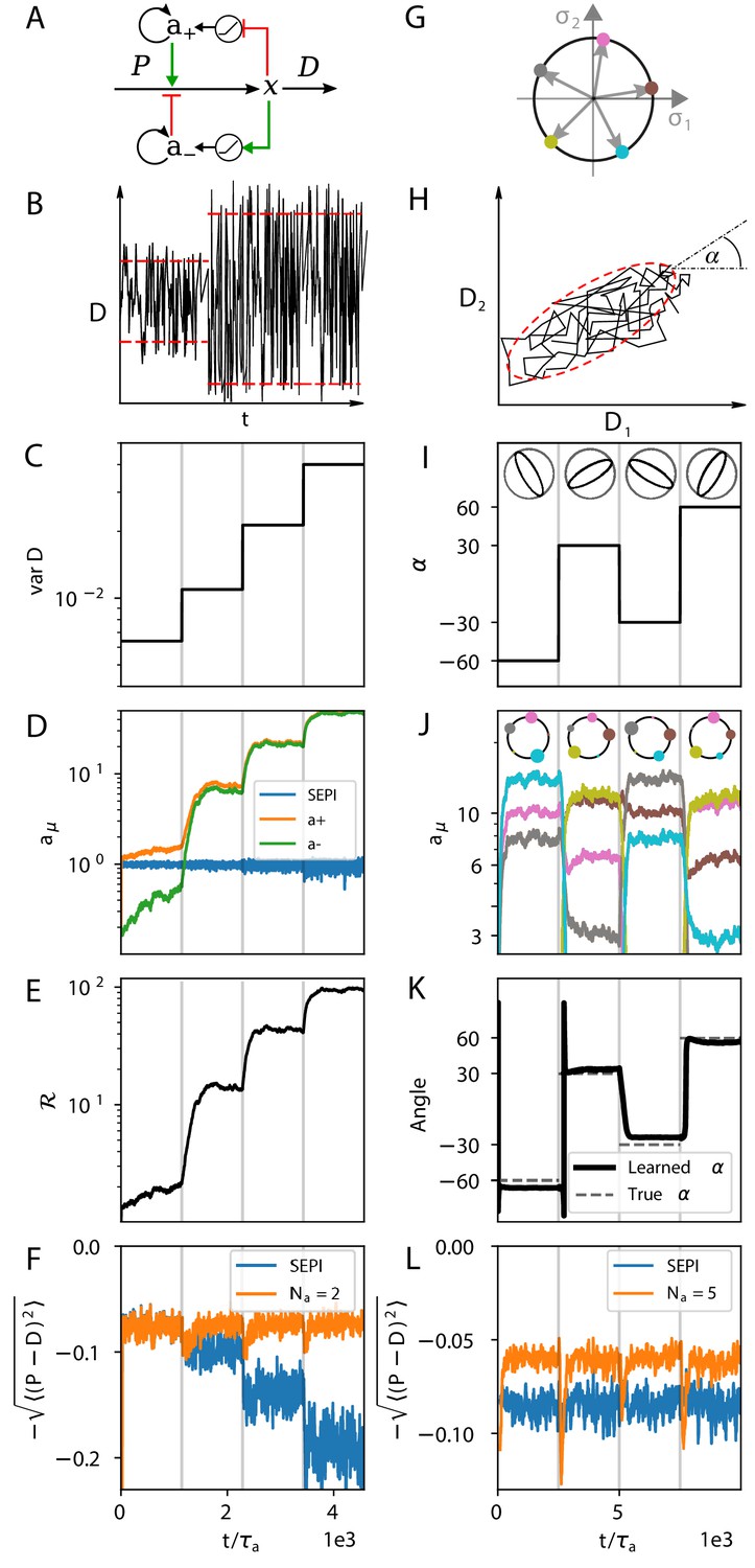
The regulatory architecture we consider successfully learns environment statistics, and outperforms simple end-product inhibition.

Left column in one dimension, right column in two. (A) Regulation of a single metabolite $x$ with one activator $a_{+}$ and one repressor $a_{-}$ . (B, C) The variance of $D$ is increased step-wise (by increasing Γ). (D) Regulator activities $a_{\pm}$ respond to the changing statistics of $\vec{D}$ . For SEPI, the activity of its single regulator is unchanged. (E) Faced with larger fluctuations, our system becomes more responsive. (F) As fluctuations increase, SEPI performance drops, while the circuit of panel A retains its performance. (G) In the 2d case, we consider a system with $N_{a} = 5$ regulators; visualization as in Figure 2D. (H) Cartoon of correlated demands with a dominant fluctuation direction (angle α). (I) We use α to change the fluctuation structure of the input. (J) Regulator activities respond to the changing statistics of $\vec{D}$ . Colors as in panel G. (K) The direction of largest responsiveness (‘learned angle’; see text) tracks the α of the input. (L) The system able to learn the dominant direction of fluctuations outperforms the SEPI architecture, even if the timescale $τ_{a}$ of SEPI is adjusted to match the faster responsiveness of the $N_{a} = 5$ system (see Appendix 1, section 'Parameters used in figures'). Panels B and H are cartoons.

Figure 4

Download asset Open asset

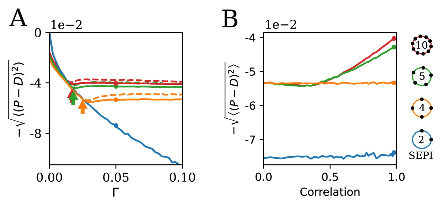
The ability to learn statistics is most useful when fluctuations are large and/or strongly correlated.

(A) The performance of different circuits shown as a function of Γ, which scales the fluctuation magnitude (input is two-dimensional and correlated, angle $α = π / 4$ , anisotropy $\sqrt{λ_{1} / λ_{2}} = 10$ ). Once the fluctuations become large enough to activate the learning mechanism, performance stabilizes; in contrast, the SEPI performance continues to decline. Arrows indicate the theoretical prediction for the threshold value of Γ; see Appendix 1, section 'The minimal Γ needed to initiate adaptation'. Dashed lines indicate the theoretical performance ceiling (calculated at equivalent Control Input Power, see text). (B) Comparison of circuit performance for inputs of the same variance, but different correlation strengths. $N_{a} = 4$ regulators arranged as shown can learn the variance but not correlation; the SEPI architecture is unable to adapt to either. Parameter Γ is held constant at 0.05; the marked points are identical to those highlighted in panel A (and correspond to fluctuation anisotropy $\sqrt{λ_{1} / λ_{2}} = 10$ ).

Figure 5

Download asset Open asset

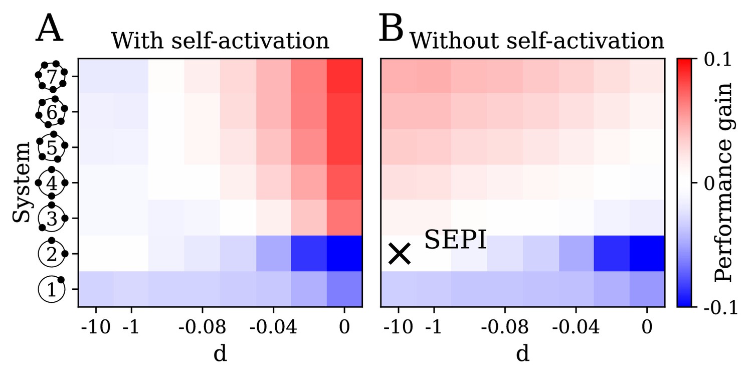
The key ingredients enabling learning are an excess of regulators, nonlinearity, and self-activation.

(A) System performance in the two-dimensional case $N_{x} = 2$ , shown as a function of the number of regulators $N_{a}$ (vertical axis) and the strength of nonlinearity $d$ (horizontal axis; $d = - 10$ is indistinguishable from a linear system with $d = - \infty$ ). Color indicates performance gain relative to the SEPI architecture; performance is averaged over angle α (see Figure 3H). (B) Same as panel A, for a model without self-activation (see text). The SEPI-like architecture (linear with $N_{a} = 2$ ) is highlighted.

Figure 6

Download asset Open asset

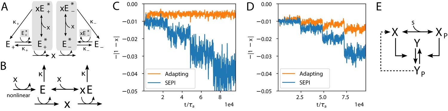
Realistic implementations.

(A) An alternative circuit that implements the logic described above, but with different forms of the key ingredients, including a Hill-function nonlinearity. Here, the circuit is based on a pair of self-activating enzymes which can be in an active ( $E^{*}$ ) or inactive state ( $E$ ). For details see Equation (5). (B) Another circuit capable of learning fluctuation variance to better maintain homeostasis of a quantity $x$ . Synthesis and degradation of $x$ are catalyzed by the same bifunctional enzyme, whose production is regulated nonlinearly by $x$ itself. For more details see Equations (6) and (7). (C) The circuit in panel A performs well at the homeostasis task of maintaining $x$ ’s concentration at 1, despite the changing variance of the input. For comparison, we’ve included a SEPI analogue of the circuit, described in Appendix 1, section 'Realistic biochemical implementations'. (D) Same as panel C, but with the circuit from panel B. Note that the ’SEPI’ line is different here, and is now a SEPI analogue of the circuit in panel B. (E) Solid arrows: a common two-component architecture of bacterial sensory systems with a bifunctional histidine kinase (X) and its cognate response regulator (Y). Adding an extra regulatory link (nonlinear auto-amplification, dashed arrow) can endow this system with self-tuned reactivity learning the statistics of the input; see text.

Appendix 1—figure 1

Download asset Open asset

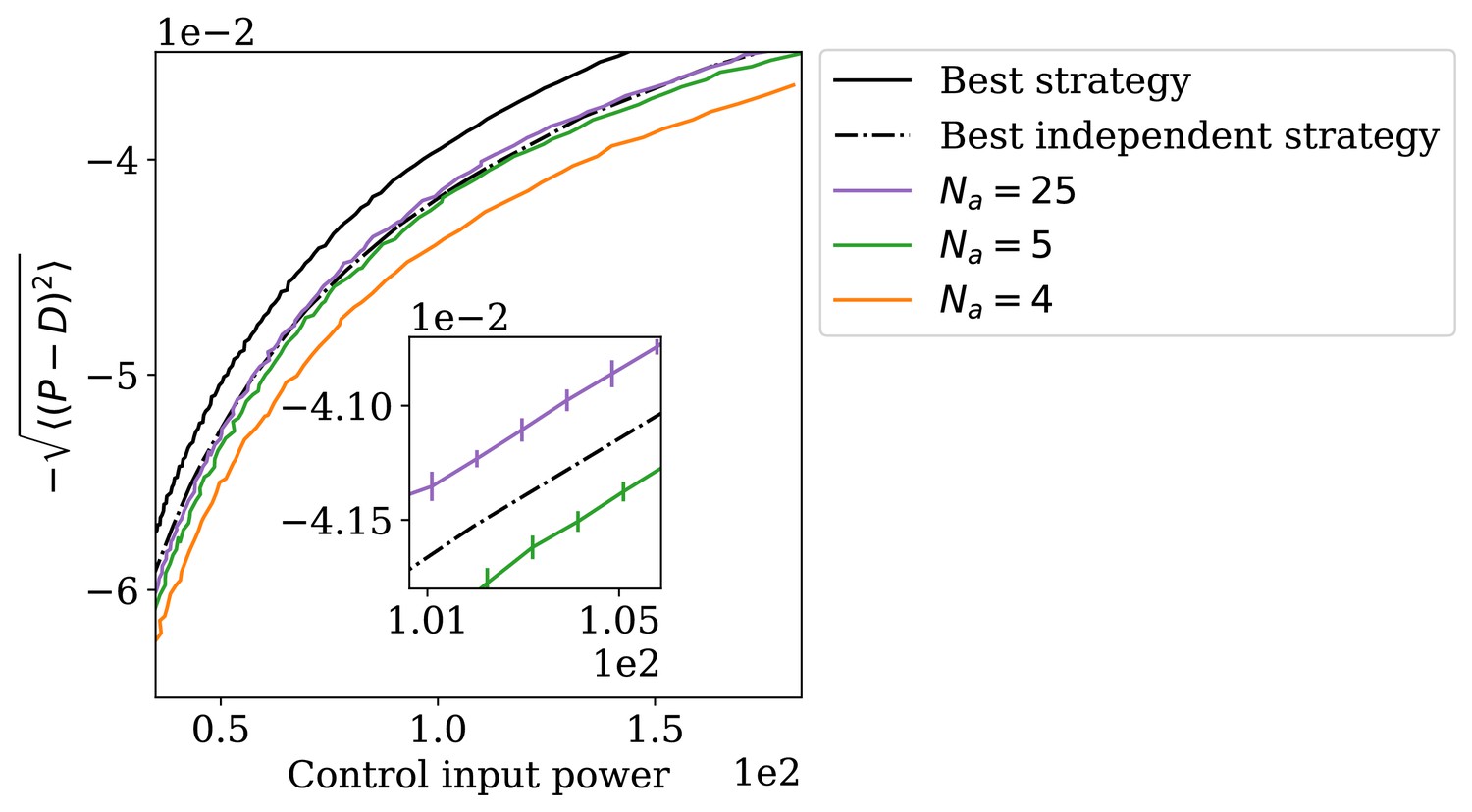
The adapting system can perform better than the best independence-assuming strategy.

Appendix 1—figure 2

Download asset Open asset

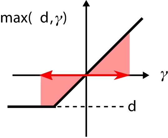
The nonlinearity in the regulatory architecture.

If the fluctuations of the input $γ = \sum_{i} σ_{μ i} (1 - x_{i})$ are large enough, the average over the nonlinearity is positive, causing additional growth of the regulator concentration $a$ .

Appendix 1—figure 3

Download asset Open asset

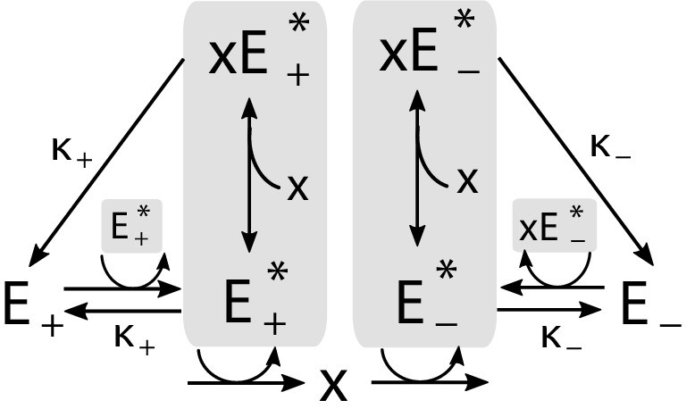
Implementation of the regulatory mechanism based on a pair of self-activating enzymes which can be in an active ( $E^{*}$ ) or inactive state ( $E$ ).

Gray shading indicates catalysts of reactions.

Appendix 1—figure 4

Download asset Open asset

Adaptation of responsiveness to an increasing variance of environmental fluctuations.

(A) Step-wise increase of the variance of $D$ . (B) Time-series of regulator concentrations, where $a_{+}$ and $a_{-}$ correspond to the total concentrations of $t_{+}$ and $t_{-}$ respectively. (C) The responsiveness of the system as defined in Equation (S31). (D) The deviation of the metabolite concentration $x$ from its target value.

Appendix 1—figure 5

Download asset Open asset

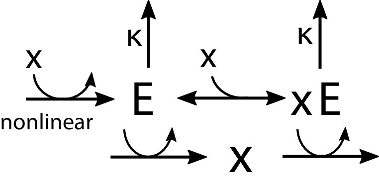
Regulation by allosteric forms of one enzyme $E$ .

The unbound form $E$ activates the production of $x$ , while the bound form $x E$ promotes its degradation. The synthesis of $E$ is regulated nonlinearly by the metabolite concentration $x$ .

Appendix 1—figure 6

Download asset Open asset

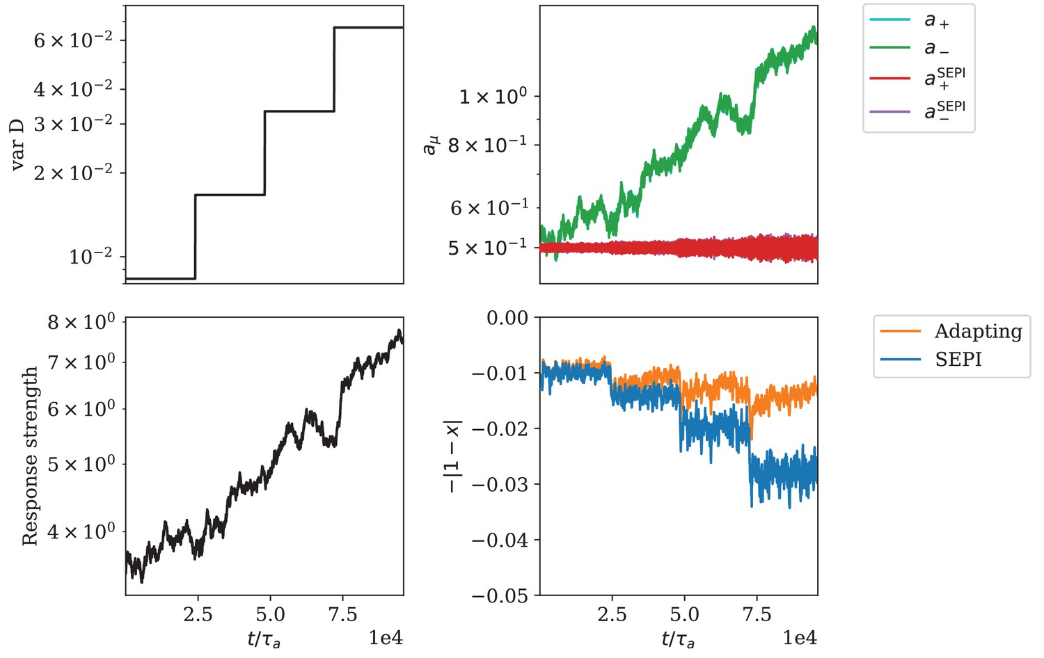
Adaptation of responsiveness for the circuit architecture based on a bifunctional enzyme.

(A) The variance of $D$ is increased step-wise. (B) Change of regulator activities. The regulator activities $a_{+}$ and $a_{-}$ overlap strongly and cannot be distinguished in this panel. (C) The response strength of the system. (D) The mismatch of the metabolite concentration $x$ from its target value.

Additional files

Source code 1 Python 3.7.4 simulation code and scripts to reproduce all figures.: https://cdn.elifesciences.org/articles/67455/elife-67455-code1-v1.zip
Download elife-67455-code1-v1.zip
Transparent reporting form: https://cdn.elifesciences.org/articles/67455/elife-67455-transrepform-v1.pdf
Download elife-67455-transrepform-v1.pdf

Download links

A two-part list of links to download the article, or parts of the article, in various formats.

Downloads (link to download the article as PDF)

Article PDF

Open citations (links to open the citations from this article in various online reference manager services)

Mendeley

Cite this article (links to download the citations from this article in formats compatible with various reference manager tools)

Stefan Landmann
Caroline M Holmes
Mikhail Tikhonov

(2021)

A simple regulatory architecture allows learning the statistical structure of a changing environment

eLife 10:e67455.

https://doi.org/10.7554/eLife.67455

Sign up for email alerts

Privacy notice