Interacting rhythms enhance sensitivity of target detection in a fronto-parietal computational model of visual attention
- Cognitive Rhythms Collaborative, Boston University, United States
- Department of Mathematics and Statistics, Boston University, United States
- Department of Neuroscience and Del Monte Institute for Neuroscience, University of Rochester Medical Center, University of Rochester, United States
- Princeton Neuroscience Institute, Princeton University, United States
- Department of Psychology, Princeton University, United States
Figures
Figure 1
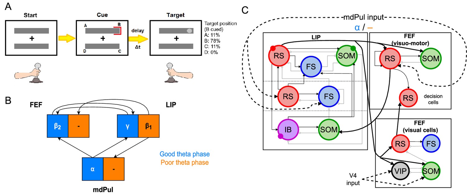
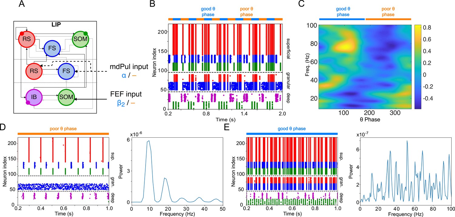
Overview of the Egly-Driver task, of the experimentally observed rhythms, and of our computational model.
(A).Schematic of the Egly-driver task modeled. (B). Neuronal rhythms experimentally measured in FEF, LIP and mdPul during the task. (C). Diagram of the full LIP and FEF model. Black lines ending in arrows and gray lines ending in circles indicate excitatory and inhibitory (chemical) synapses, respectively. Thick lines indicate synapses between modules. Dashed lines indicate synthetic inputs from regions that are not modeled. Circles indicate gap junctions between population neurons. The mdPul input is at an α frequency during the good θ phase and is absent in the poor θ phase. RS: regular spiking pyramidal neurons. IB: intrinsic bursting pyramidal neurons. FS: fast-spiking (e.g. parvalbumin-positive) inhibitory interneurons. SOM: somatostatin-positive interneurons. VIP: vasoactive intestinal peptide-positive interneurons.
Figure 2
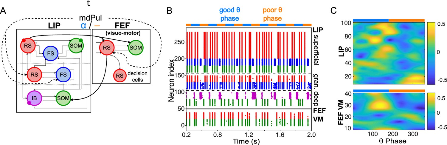
Model activity during the cue-target interval.
(A). Diagram of the interconnected LIP and FEF visuomotor modules. Symbols are as in Figure 1C. (B). The LIP and FEF visuomotor modules reproduce experimentally observed rhythms when driven by mdPul. Raster plot from a 2 s long simulation with an alternation of good and poor θ phase pulvinar inputs. The activity of LIP is shown on top, and that of the FEF visuomotor module at the bottom. No target was presented, so decision-cells were quiescent and are omitted. C. Spectral power as a function of θ phase for simulation shown in B. LIP produces an alternation of γ and rhythms. FEF visuomotor cells produce oscillations only during the good θ phase. Simulated LFP obtained from the sum of RS membrane voltages. See Methods for details.
Figure 3
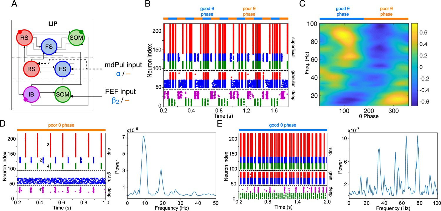
LIP module activity during the cue-target interval.
(A). Diagram of the LIP module. Symbols are as in Figure 1C. (B). LIP module spiking during a 2 s long simulation with synthetic pulvinar and FEF inputs. (C). Spectral power as a function of θ phase for the simulation shown in (B). Simulated LFP obtained from the sum of RS membrane voltages. See Methods for details. (D). Reproduction of LIP rhythm characteristic of the poor θ phase. Left, raster plot of a 1 second simulation of LIP activity with no input, corresponding to the poor θ phase, showing a oscillatory rhythm obtained through period concatenation. A single cycle of this rhythm is labeled: 1, IB cells spike by rebound; 2, superficial FS cells spike in response to IB excitation; 3, superficial RS cells spike by rebound; 4, superficial SOM cells spike in response to RS excitation. Right, power spectrum of the LFP generated by superficial RS cells for the same simulation, with a peak in the frequency band. (Note that this simulation is half as long as those shown in B and E, to clearly show the structure of the oscillation.) (E). Reproduction of LIP γ rhythm, characteristic of the good θ phase. Left, raster plot of a 2 s simulation of LIP activity in the presence of inputs, corresponding to the good θ phase, showing γ rhythms in the granular and superficial layers. Right, power spectrum of the LFP generated by superficial RS cells for the same simulation, with peaks in the γ frequency band.
Figure 4
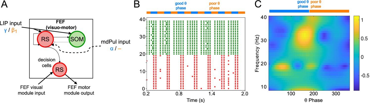
FEF visuomotor cell activity during the cue-target interval.
(A). Diagram of the FEF visuomotor module. Symbols are as in Figure 1C. (B). Raster plot of a 1s-long simulation of FEF visuomotor cells with synthetic input. mdPul α input during the good θ phase alters the E-I balance, enabling RS and SOM cells to form a rhythm. No target was presented, so decision-cells were quiescent and are omitted. (C). Spectral power as a function of θ phase for simulation shown in B. Simulated LFP obtained from the sum of RS membrane voltages. See Methods for details.
Figure 5
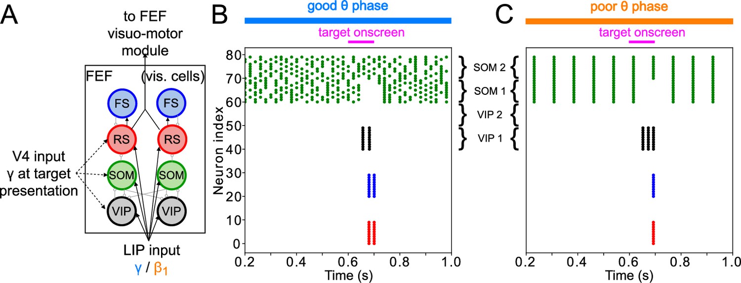
FEF visual module activity at target presentation.
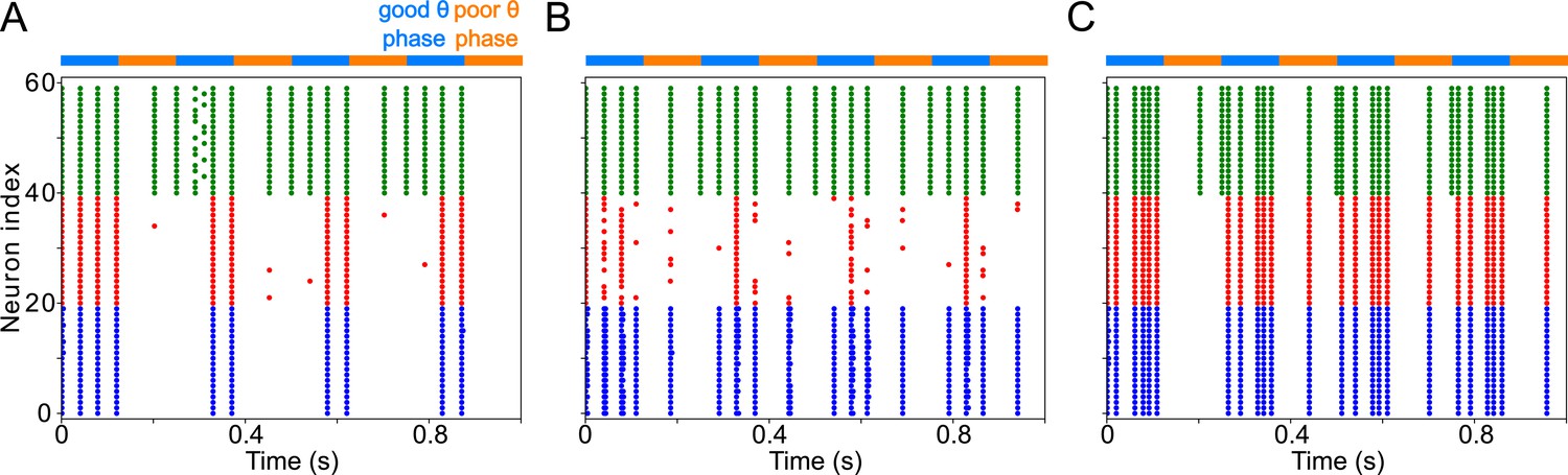
(A) Diagram of the FEF visual module. Symbols are as in Figure 1C. (B). Raster plot of a 1s-long simulation of FEF visual cells with good θ phase LIP input. A target appears on screen at for a duration of , producing two cycles of γ in RS and FS cells. (C). Raster plot of a 2 s simulation of FEF visual cells with poor θ phase LIP input. A target appears on screen at for a duration of , producing a single volley of RS spikes.
Figure 6
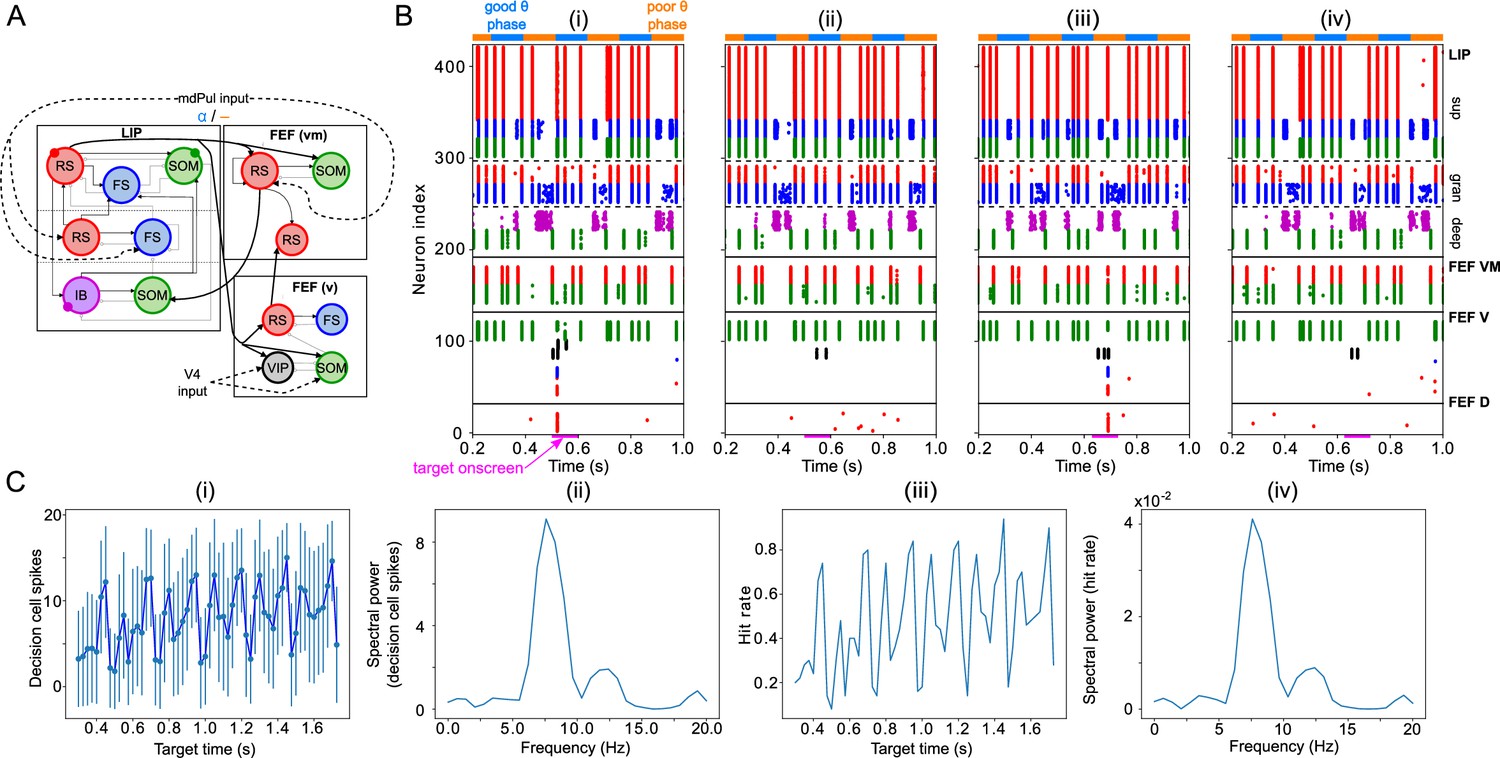
Model activity in response to target presentation.
(A). Diagram of the model. Symbols are as in Figure 1C. (B). Raster plots of the model during a 1 s long simulation with simulated mdPul input and target presentation during the good or poor θ phase. The raster plots show activity of LIP on top, that of FEF visuomotor cells right below, that of FEF visual cells below them, and that of FEF decision cells at the bottom. A target was presented for 100ms in the good θ phase in (i) and (ii), and in the poor θ phase in (iii) and (iv). Only in (i) and (iii) did target presentation lead to a ‘hit’. (C). Decision cell activity and hit rate depend on θ phase. (i) Number of decision cells spikes (with mean and standard deviation) during target appearance as a function of the cue-target interval. (ii) Power spectrum of decision cell spiking, showing a peak at a θ frequency (8 Hz). (iii) Hit rate as a function of the cue-target interval. (iv) Power spectrum of the hit rates, showing a peak at a θ frequency (8 Hz).
Figure 7
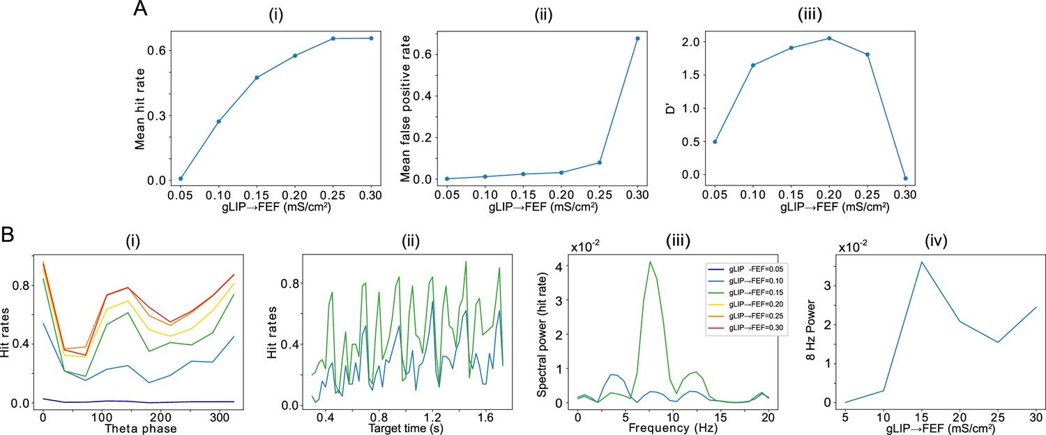
Effect of the strength of LIP -> FEF chemical synapses on network sensitivity and hit rates rhythmicity.
(A).The strength of LIP → FEF chemical synapses influences network sensitivity. (i) Hit rate as a function of . (ii) False alarm rate as a function of . (iii) D’ as a function of . (B). Increased leads to a stronger 8 Hz component in the hit rates. (i) Hit rate as a function of θ phase plotted for values of between 0.05 and 0.3. (ii) Hit rate as a function of the cue-target interval for and . (iii) Power spectra of the hit rate time series shown in (ii). (iv) 8 Hz power as a function of .
Figure 8
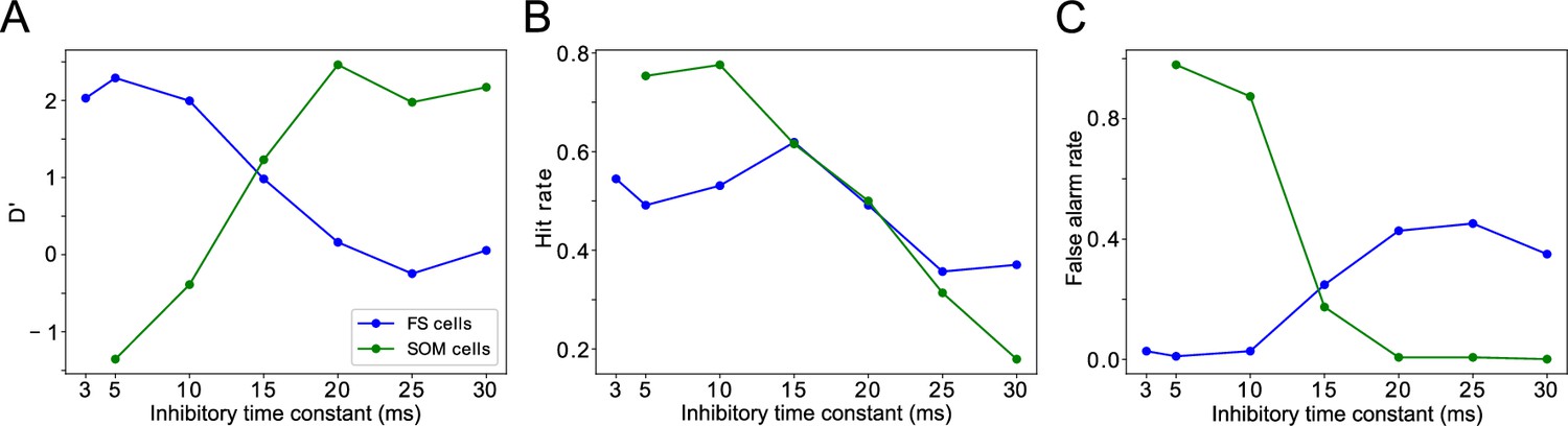
Changing timescales of FEF and LIP rhythmic dynamics negatively impacts task performance.
(A). D’ measure as a function of the time constants of inhibition for SOM cells and FS cells. (B). Hit rate as a function of the time constants of inhibition for SOM cells and FS cells. (C). False alarm rate as a function of the time constants of inhibition for SOM cells and FS cells.
Figure 9
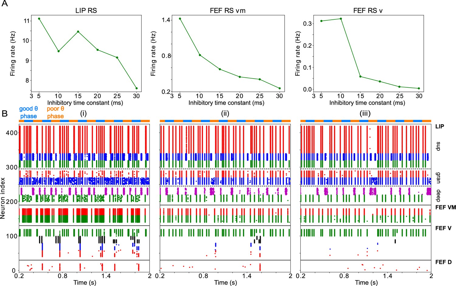
Changing impacts network dynamics and function.
(A) The firing rates of RS cells in the LIP, FEF visuomotor, and FEF visual modules as a function of . (B) Raster plots of network activity for three values of : (i) ms, showing several false alarms; (ii) ms, showing a hit; (iii) ms, showing a miss.
Figure 10
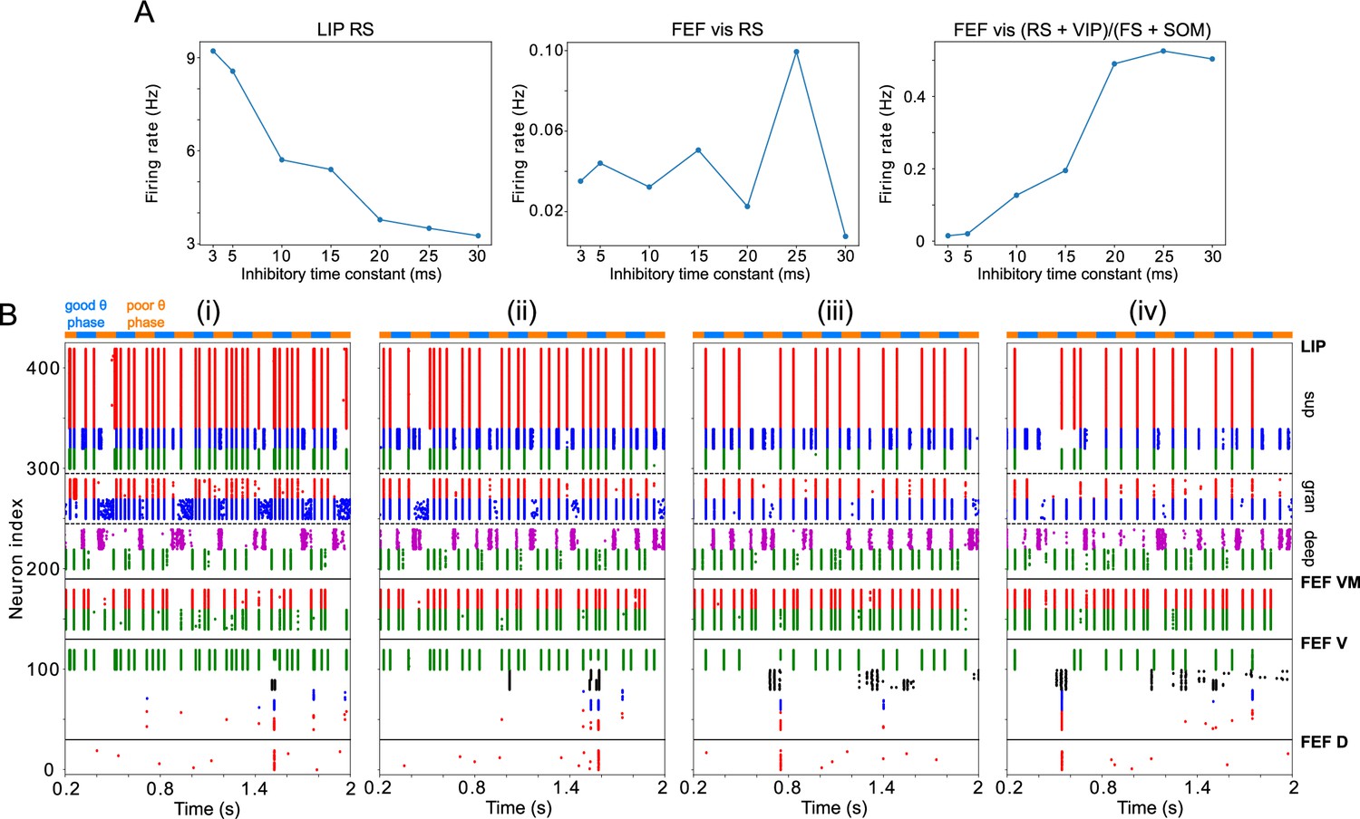
Changing impacts network dynamics and function.
(A) The firing rates of RS cells in the LIP superficial layer and the FEF visual module, and the sum of excitatory and disinhibitory spike rates divided by inhibitory spike rates, as a function of . (B) Raster plots of network activity for four values of : (i) ms (showing a hit); (ii) ms (showing a hit); (iii) ms (showing a false alarm); (iv) ms (showing a false alarm).
Figure 11
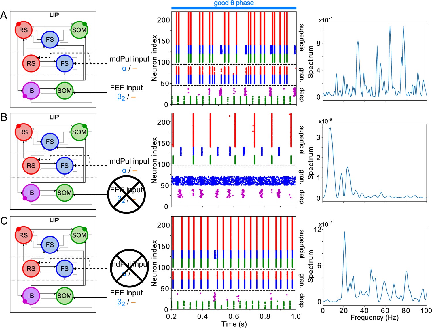
LIP good θ phase behavior depends on mdPul and FEF inputs.
(A). LIP good θ phase behavior with both mdPul and FEF inputs. (B). LIP good θ phase behavior with FEF input but no mdPul input. (C). LIP good θ phase behavior with mdPul input but no FEF input. Columns are as follows: Left, diagram of the model. Symbols are as in Figure 1C. Middle, raster plot of a 1s-long simulation. Right, power spectrum of the LFP generated by the network in this 1s-long simulation.
Figure 12
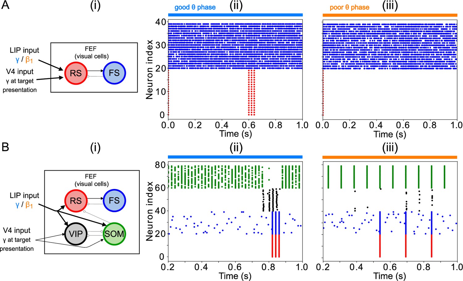
Modeling choices in the FEF visual module.
(A). A model without VIP and SOM cells fails to detect a small change in input. (i) Diagram of FEF visual module without VIP and SOM cells. Symbols are as in Figure 1C. (ii) Raster plot of a 1 s simulation of the model with a target input applied between 600ms and 700ms at 1.5 times the strength of the background input, producing a γ burst in RS cells. (iii) Raster plot of a 1 s simulation of the model with a target input applied between 600ms and 700ms at 0.5 times the strength of the background input, producing no activity in RS cells. (B). A model with a single population leads to false alarms in the poor θ phase. Panel (i) as above. (ii) Raster plot of a 1 second simulation of the model with good θ phase inputs, and target input applied between 600ms and 700ms, leading to γ activity in RS cells only during target presentation. (iii) Raster plot of a 1 s simulation of the model with poor θ phase inputs, and target input applied between 600ms and 700ms, leading to RS cell activity outside of target presentation.
Appendix 1—figure 1
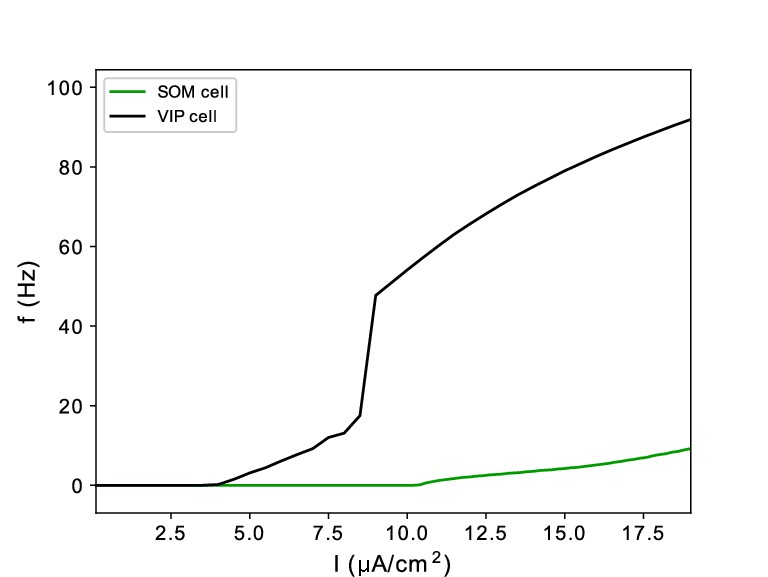
f-I curves of model SOM and VIP cells.
Appendix 1—figure 2
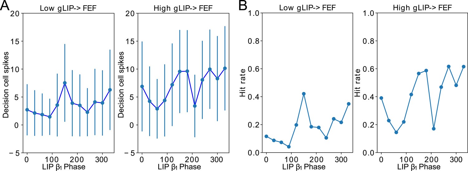
Conductance of LIP → FEF synapses increases dependence of decision cell spiking and hit rate on LIP phase.
(A). Decision cell spiking (mean±SD) as a function of LIP phase (see Methods). (B). Hit rate as a function of LIP phase.
Appendix 1—figure 3

The power of 8 Hz rhythmicity in hit-rate depends on mdPul input increasing across the good θ phase.
Simulation results as in Figure 7 are shown for a network with mdPul input of constant maximal conductance. (A). Increased leads to a stronger 8Hz component in the hit rates. (i) Hit rate as a function of θ phase plotted for values of between 0.05 and 0.3 (see (iii) for legend). (ii) Hit rate as a function of the cue-target interval for and (iii) Power spectra of the hit rate time series shown in (ii). (iv) 8 Hz power as a function of (B). Network sensitivity as a function of LIP → FEF connectivity. (i) Hit rate as a function of (ii) False alarm rate as a function of (iii) D’ as a function of .
Appendix 2—figure 1
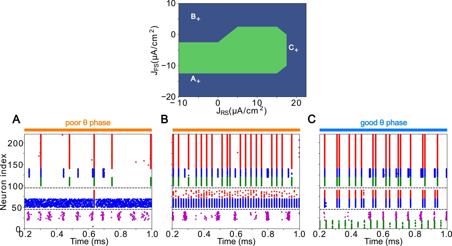
LIP good and poor θ phase behavior depends on input layer tonic excitation.
Top: Appropriate tonic excitation range needed to obtain a γ rhythm in the good θ phase and rhythm in the poor θ phase. The crosses indicate the sets of values used in simulations for (A, B, and C) below. (A). Excessive tonic excitation to input layer FS cells disturbs the poor θ phase rhythm by preventing superficial RS cells spikes. (B). Insufficient tonic excitation to input layer FS cells disturbs the poor θ phase rhythm by allowing input RS cells to spike and entrain the superficial layer. (C). Insufficient tonic excitation to input layer RS cells disturbs the good θ phase γ rhythm.
Appendix 2—figure 2
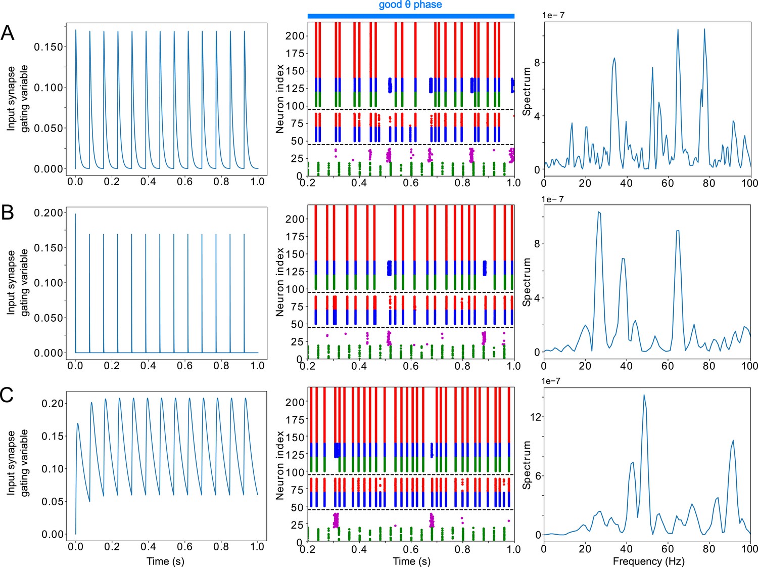
LIP good θ phase γ can be obtained with mdPul α stimulation of various widths.
(A). LIP good θ phase behavior with mdPul input synapse timescales of and , the default values used throughout this paper. Left: input synapse opening variable of a 1s-long simulation. Middle: Raster plot of a 1s-long simulation. Right: power spectrum of the LFP generated by the network in this 1s-long simulation. (B). LIP good θ phase behavior with shorter mdPul input synapse timescales of and . Subplots are as described for A. (C). LIP good θ phase behavior with longer mdPul input synapse timescales of and . Subplots are as described for A.
Appendix 3—figure 1

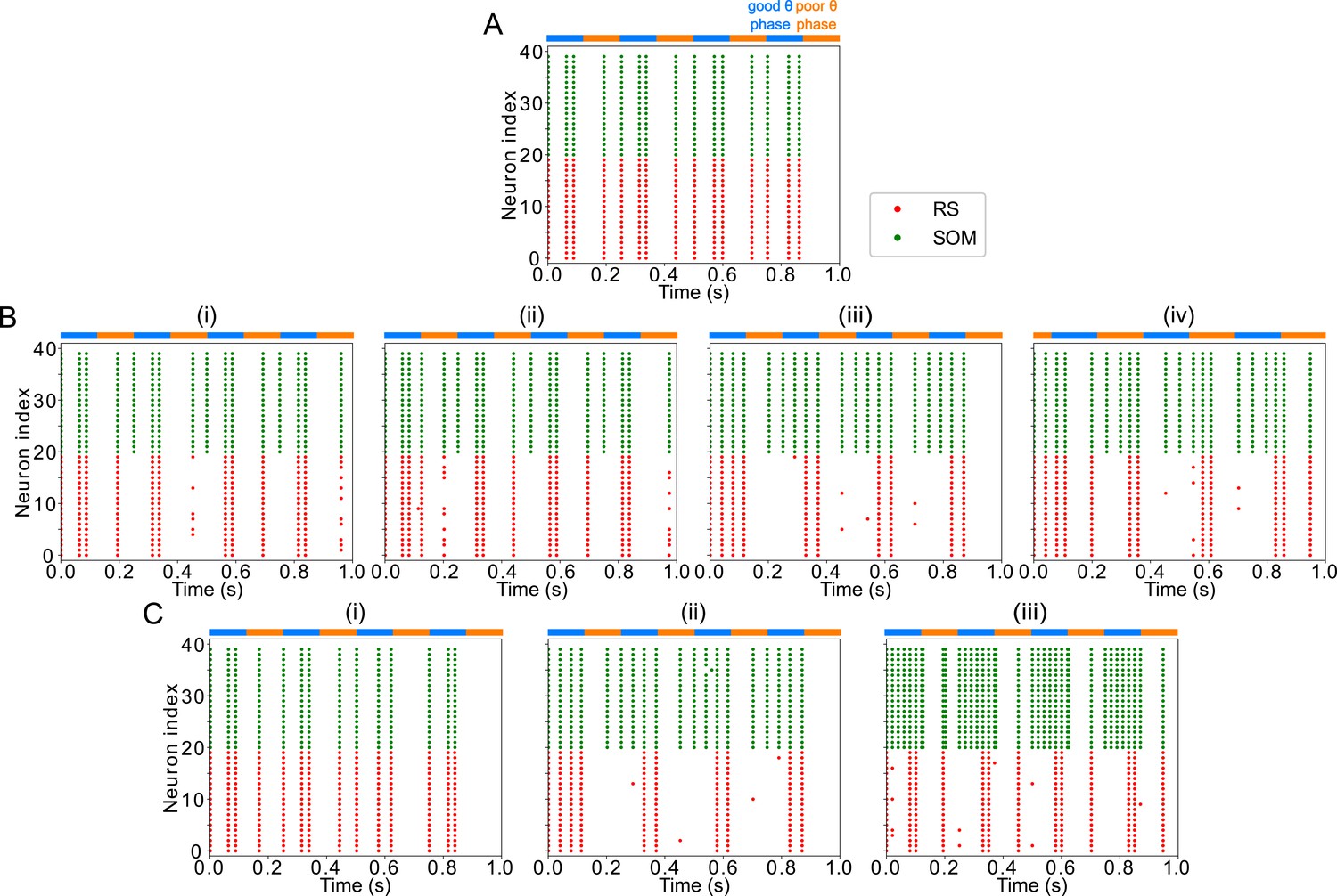
FEF visuomotor module good θ phase behavior is influenced by mdPul input properties.
(A). Raster plot of FEF visuomotor behavior without mdPul input during a 1s-long simulation with alternating good and poor θ phase (no rhythm appears in the good θ phase). (B). Raster plots of FEF visuomotor behavior with various mdPul input frequencies, during a 1s-long simulations with alternating good and poor θ phase. Left: 5 Hz mdPul input (the rhythm is not sustained). Middle: 13 Hz mdPul input (the rhythm is preserved). Right: 30Hz mdPul input (the rhythm is speeds up). (C). Raster plot of FEF visuomotor good θ phase behavior with altered mdPul input synapse timescales. Left: and (the rhythm is not preserved). Right: and (the rhythm is not preserved). (D). Raster plots of FEF visuomotor behavior, during a 1s-long simulations with alternating good and poor θ phase with various frequencies. Left: 2Hz "θ" input, with linearly increasing maximal conductance, and with increasing then decreasing maximal conductance (the good θ phase is mostly preserved, with spikes appearing during the poor θ phase). Right: 8Hz "θ" input with the same maximal conductance as the low and high amplitude 4 Hz pulses.
Appendix 3—figure 2
FEF visuomotor module good θ phase behavior is influenced by LIP input properties.
(A). Raster plot of FEF visuomotor behavior without LIP input during a 1s-long simulation with alternating good and poor θ phase (the good θ phase rhythm is altered and spikes appear in the poor θ phase). (B). Raster plots of FEF visuomotor behavior with various LIP input frequencies during 1s-long simulations with alternating good and poor θ phase. (i) 5Hz LIP input speeds the good θ phase rhythm. (ii) 13Hz LIP input speeds the good θ phase rhythm. (iii) 25Hz LIP input preserves the good θ phase rhythm. (iv) 150Hz LIP input speeds the good θ phase rhythm. (C). Raster plots of FEF visuomotor behavior with various LIP input strengths during 1s-long simulations with alternating good and poor θ phase. (i) input. (ii) input. (iii) input.
Appendix 3—figure 3
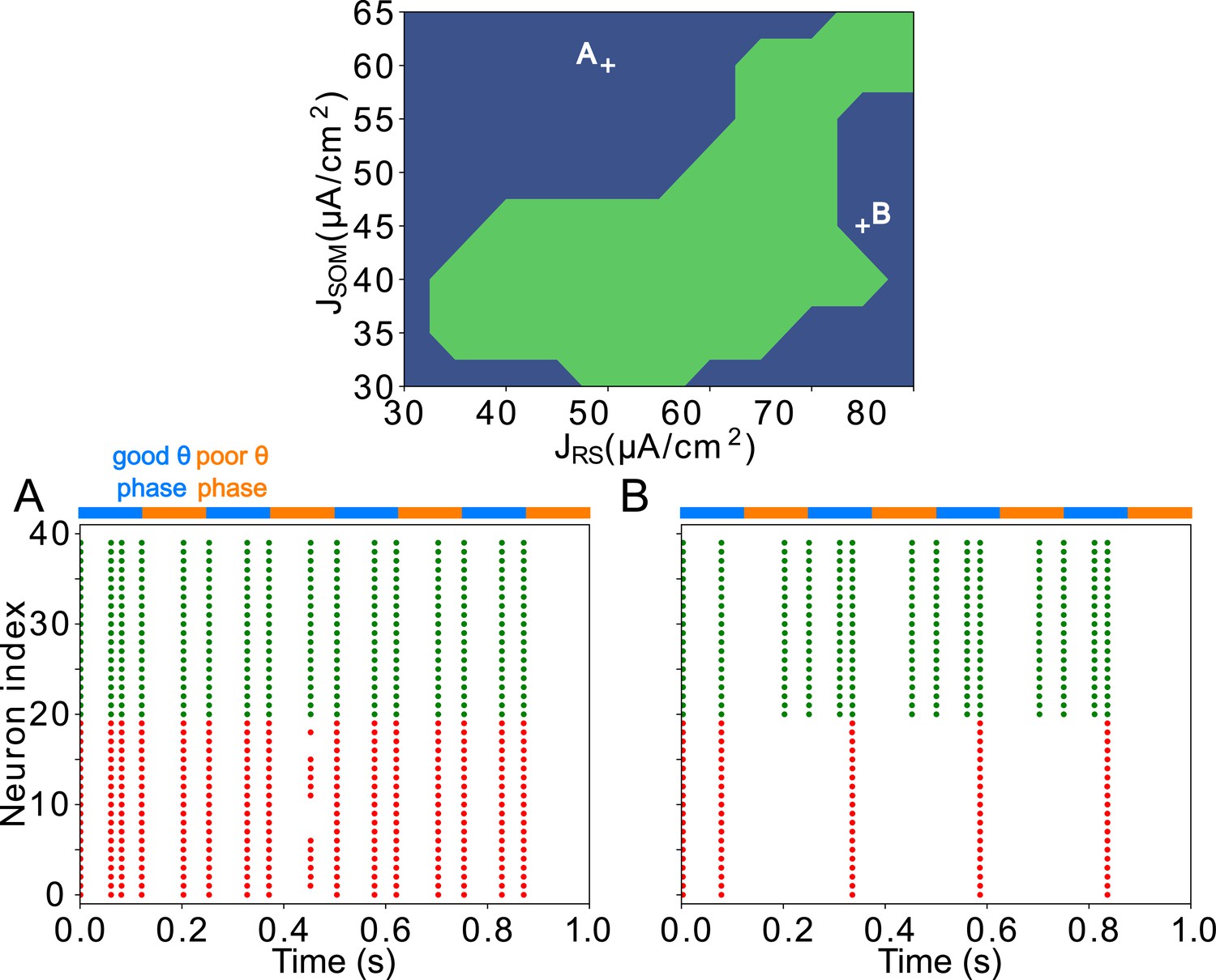
FEF visuomotor module good and poor θ phase behavior depends on the tonic excitation given to RS and SOM cells Top: Appropriate tonic excitation range needed to obtain a rhythm in the good θ phase and quiet RS cells in the poor θ phase.
The crosses indicate the two sets of values used in simulations for A and B below. (A). Insufficient tonic excitation to SOM cells disturbs the poor θ phase by allowing RS cells spikes. (B). Excessive tonic excitation to SOM cells disturbs the good θ phase rhythm by silencing RS cells outside the windows of excitation provided by mdPul.
Appendix 4—figure 1
LIP module behavior persists with the addition of recurrent connections between RS cells.
(A). Diagram of the LIP module with recurrent RS synapses. Recurrent synapses between RS cells have the same maximal conductance as RS→FS synapses, 1/40. Symbols are as in Figure 1C. (B). LIP module spiking during a 1-second long simulation with synthetic pulvinar and FEF inputs. (C). Spectral power as a function of θ phase for the LIP module. Simulated LFP obtained from the sum of RS membrane voltages. See Methods. (D). Reproduction of LIP oscillatory rhythm, characteristic of the poor θ phase. Left, raster plot of a 1-second simulation of LIP activity with no input, corresponding to the poor θ phase, showing a oscillatory rhythm obtained through period concatenation. A single cycle of this rhythm is labeled: 1, IB cells spike by rebound; 2, superficial FS cells spike in response to IB excitation; 3, superficial RS cells spike by rebound; 4, superficial SOM cells spike in response to RS excitation. Right, power spectrum of the LFP generated by superficial RS cells for the same simulation, with a peak in the frequency band. (E). Reproduction of LIP γ oscillatory rhythm, characteristic of the good θ phase. Left, raster plot of a 1-second simulation of LIP activity in the presence of inputs, corresponding to the good θ phase, showing γ rhythms in the granular and superficial layers. Right, power spectrum of the LFP generated by superficial RS cells for the same simulation, with a peak in the γ frequency band.
Appendix 4—figure 2
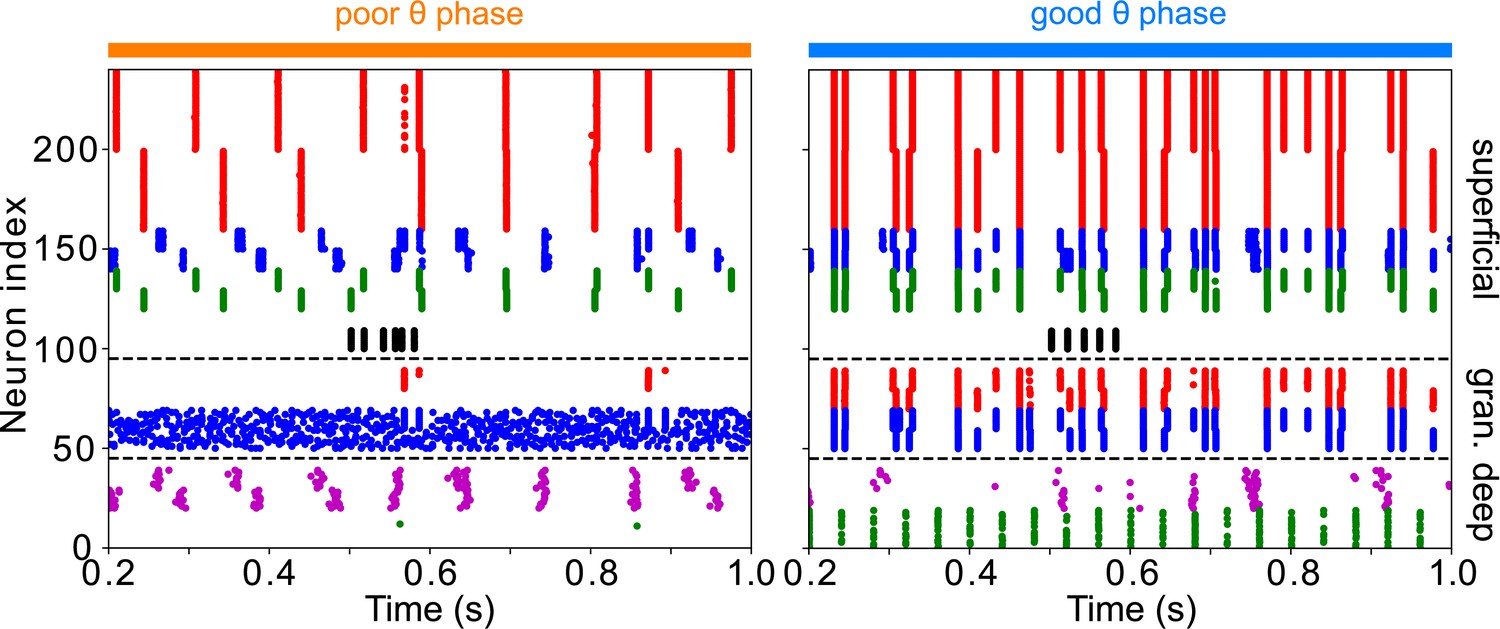
The addition of VIP interneurons to form a target-detection module in LIP superficial layer does not alter the network response to low-contrast targets.
Simulations are for LIP superficial layer with the addition of VIP interneurons, connected to RS, FS, and SOM cells as in the FEF visual module, but receiving target input twice as strong. During the poor θ phase, target input delays firing of superficial RS cells; during the good θ phase, target input has no discernable effect on superficial RS cell firing.
Appendix 4—figure 3
FEF visuomotor module behavior persists with the addition of an FS cell population, provided FS inhibition is not stronger than SOM inhibition.
(A). Setting the conductance of synapses between the RS and FS population at the same level as synapses between RS and SOM cells preserves the rhythm in FEF. ( , ). (B). Increasing the conductance of the synapse between the RS and FS populations reduces RS spiking and abolishes the rhythm. ( , , , .) (B). Decreasing the conductance of the synapses from SOM to RS populations shifts the frequency of RS spiking to a γ rhythm (arising through a typical PING mechanism). ( , , .).
Tables
Table 1
Ion channel parameters for RS cells.
| Channel | ( ) | ( ) | (ms) | (ms) | ||||
|---|---|---|---|---|---|---|---|---|
| L | 1 | –70 | 0 | 0 | - | - | - | - |
| Na | 200 | 50 | 3 | 1 | - |
|
|
|
| K | 20 | –95 | 4 | 0 |
|
- | - | |
| h | 25 | –35 | 1 | 0 |
|
- | - |
Table 2
Ion channel parameters for FS cells.
| Channel | ( ) | ( ) | ||||||
|---|---|---|---|---|---|---|---|---|
| L | 1 | –65 | 0 | 0 | - | - | - | - |
| Na | 200 | 50 | 3 | 1 | - |
|
|
|
| K | 20 | –100 | 4 | 0 |
|
- | - |
Table 3
Ion channel parameters for SOM cells.
| Channel | ( ) | ( ) | ||||||
|---|---|---|---|---|---|---|---|---|
| L | 6 | –65 | 0 | 0 | - | - | - | - |
| Na | 200 | 50 | 3 | 1 | - |
|
|
|
| K | 10 | –100 | 4 | 0 |
|
- | - | |
| h | 50 | –35 | 1 | 0 |
|
- | - |
Table 4
Ion channel parameters for VIP cells.
| Channel | ( ) | ( ) | ||||||
|---|---|---|---|---|---|---|---|---|
| L | 0.25 | –70 | 0 | 0 | - | - | - | - |
| Na | 112.5 | 50 | 3 | 1 | - |
|
|
|
| K | 225 | –90 | 2 | 0 |
|
- | - | |
| D | 4 | –90 | 3 | 1 | 2 |
|
150 |
|
Table 5
Ion channel parameters for IB cells.
| Channel | ( ) | ( ) | ||||||
|---|---|---|---|---|---|---|---|---|
| L | 2 (a.d., b.d.) 1 (soma) 0.25 (axon) |
–70 | 0 | 0 | - | - | - | - |
| Na | 125 (a.d., b.d.) 50 (soma) 100 (axon) |
50 | 3 | 1 | - |
|
|
|
| K | 10 (a.d., b.d., soma) 5 (axon) |
–95 | 4 | 0 |
|
- | - | |
| h | 155 (a.d.) 115 (b.d) |
–25 | 1 | 0 |
|
- | - | |
| Channel |
( ) |
( ) |
||||||
| M | 0.75 (a.d., b.d) 1.5 (axon) |
–95 | 1 | 0 |
|
|
- | - |
| CaH | 6.5 (a.d, b.d) | 125 | 2 | 0 |
|
- | - |
Table 6
Random input amplitude for each cell type.
| Cell Type | Noise Amplitude |
|---|---|
| RS | 0.075 |
| FS | 0.025 |
| SOM | 0.025 |
| VIP | 0 |
| IB (axon) | 0.0125 |
| IB (soma) | 0 |
| IB (apical dendrites) | 0.0025 |
| IB (basal dendrites) | 0.0025 |
Table 7
Synaptic reversal potentials and time constants for each synapse type in the network.
| Synapse type | Source neuron | |||
|---|---|---|---|---|
| AMPA | RS, IB | 0 mV | 0.125ms | 1ms |
| NMDA | RS | 0 mV | 12.5ms | 125ms |
| GABA (fast inhibition) | FS | –80 mV* | 0.25ms | 5ms |
| GABA (slow inhibition) | SOM, VIP | –80 mV | 0.25ms | 20ms |
-
*
FS to FS synapses have a –75 mV reversal potential, instead of –80 mV.
Table 8
Maximum conductances of the synapses in the network (in ).
| Source region | LIP | FEF vm | FEF v | |||||||||||
|---|---|---|---|---|---|---|---|---|---|---|---|---|---|---|
| Neuron | RS | FS | SOM | g.RS | g.FS | IB | d.SOM | RS | SOM | RS | FS | SOM | VIP | |
| Target region | Neuron | |||||||||||||
| LIP | RS FS SOM g.RS g.FS IB d.SOM |
- 0.025 0 .225 - - 1 /60* - |
6.25 2 0.4 - - - - |
2 0.2 7 - - 0.4 - |
2 0.1 - 0.5 1 - - |
0.1 - - 1 0.3 - - |
- 0.08 0.045 - - 1/500 - |
- - - - 1 10 - |
- - - - - - 0.05 |
- - - - - - - |
- - - - - - - |
- - - - - - - |
- - - - - - - |
- - - - - - - |
| FEF vm | RS SOM |
0.009 0.009 |
- - - |
- - - |
- - - |
- - - |
- - - |
- - - |
0.6 0.5 - |
0.8 - - |
- - - |
- - - |
- - - |
- - - |
| FEF v | RS FS SOM VIP |
0.015 - 0.025 0.005 |
- - - - |
- - - - |
- - - - |
- - - - |
- - - - |
- - - - |
- - - - |
- - - - |
0.2 0.2 - - |
0.2 0.2 - - |
1 - - 0.01 |
- - 0.7 - |
| FEF m | RS | - | - | - | - | - | - | - | 0.1 † | - | 0.08 ‡ | - | - | - |
-
*
For AMPA synapse. For NMDA : gi = 1∕240.
-
†
For AMPA synapse. For NMDA : gi = 0.01.
-
‡
*For NMDA synapse. For AMPA : gi = 0.
Table 9
Conductances of gap junctions between IB cell compartments.
| Source compartment | Target Compartment | |
|---|---|---|
| Soma | Apical Dendrite | 0.2 |
| Soma | Basal Dendrite | 0.2 |
| Soma | Axon | 0.3 |
| Apical Dendrite | Soma | 0.4 |
| Basal Dendrite | Soma | 0.4 |
| Axon Dendrite | Soma | 0.3 |
Table 10
Nominal frequency and maximum conductances (in ) of inputs to the model, coming from mdPul, LIP, FEF or V4.
The two conductance values given for mdPul inputs are for the first and second input volleys occurring during each good θ phase.
| Parameter | mdPul input | LIP input(only when FEF ismodeled alone) |
FEF input(only when LIP ismodeled alone) |
V4 input(only duringtarget appearance) |
|---|---|---|---|---|
| Good theta | 13 Hz | 50 Hz | 25 Hz | 50 Hz |
| Poor theta | - | 13 Hz | - | 50 Hz |
| to LIP gran. RS: 2.5/5 to LIP gran. FS: 2.5/5 to FEF vm RS: 2.5/5 to FEF vm SOM: 3 |
to FEF vm RS : 3 to FEF vm SOM : 3 to FEF v VIP : 2.5 to FEF v SOM : 7.5 to FEF v RS : 7.5 |
to LIP deep SOM : 5 | to FEF v VIP : 3 to FEF v SOM : 2.5 |
Additional files
Download links
A two-part list of links to download the article, or parts of the article, in various formats.
Downloads (link to download the article as PDF)
Open citations (links to open the citations from this article in various online reference manager services)
Cite this article (links to download the citations from this article in formats compatible with various reference manager tools)
Interacting rhythms enhance sensitivity of target detection in a fronto-parietal computational model of visual attention
eLife 12:e67684.
https://doi.org/10.7554/eLife.67684


