Genetic variation, environment and demography intersect to shape Arabidopsis defense metabolite variation across Europe
- Department of Plant Sciences, University of California, Davis, United States
- Gregor Mendel Institute, Austrian Academy of Sciences, Vienna Biocenter (VBC), Austria
- Department of Molecular Biology, Max Planck Institute for Developmental Biology, Germany
- Division of Biological Sciences, Bond Life Sciences Center, University of Missouri, United States
- Division of Biological Sciences, Interdisciplinary Plant Group, Christopher S. Bond Life Sciences Center, University of Missouri, United States
- DynaMo Center of Excellence, University of Copenhagen, Denmark
Figures
Figure 1
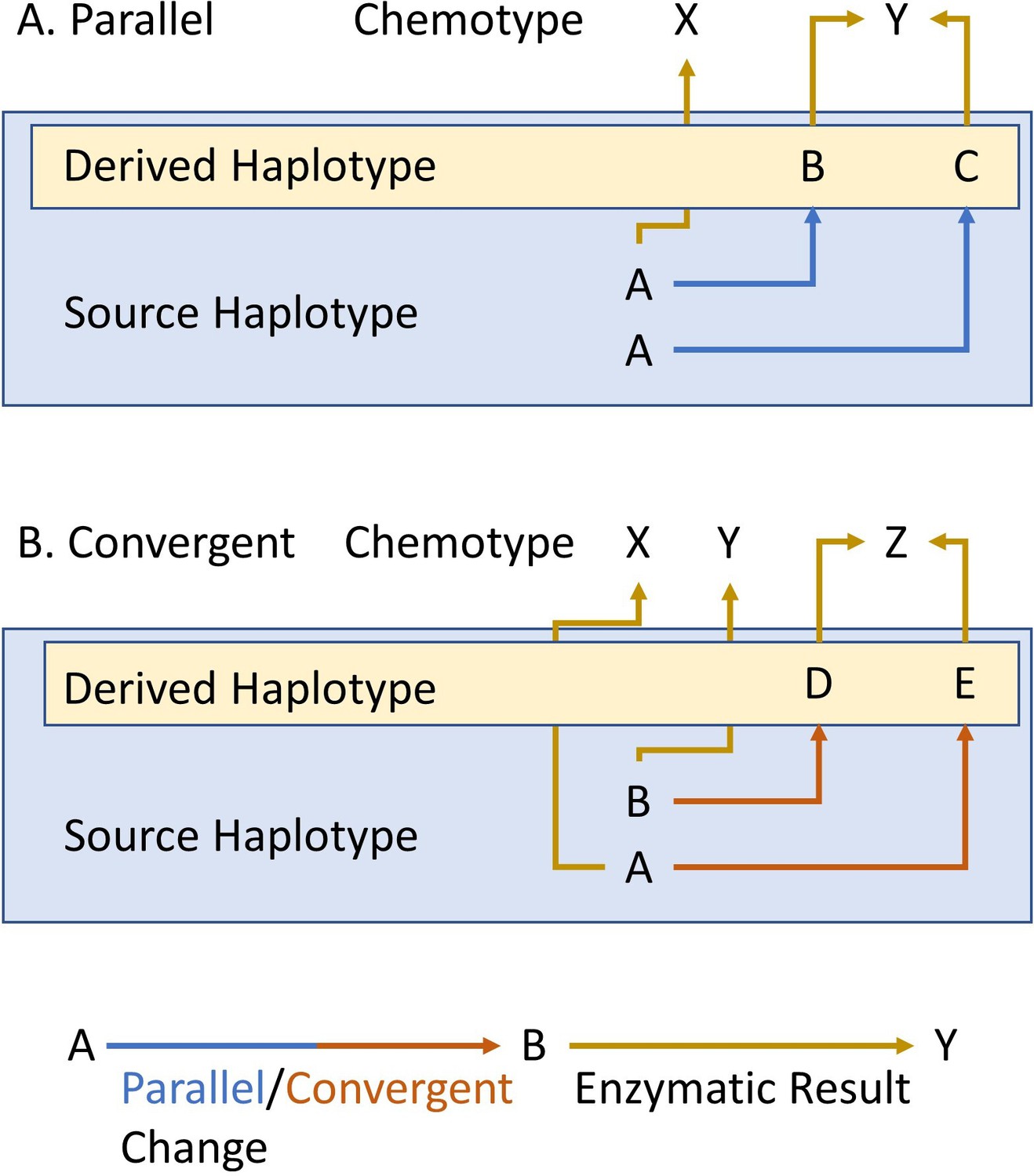
Parallel and convergent evolution.
The schema describes our use of parallel (A) and convergent (B) evolution for within-species chemotypic variation. The letters in the blue box represent the state of the source/ancestral haplotypes. The letters within the yellow box represent the newly derived haplotypes that arose by genetic mutation in the source haplotype. Finally, X, Y and Z show the chemotypes that arise from each haplotype. Blue and red arrows represent parallel or convergent genetic changes (respectively), while mustard arrows represent the enzymatic result.
Figure 2
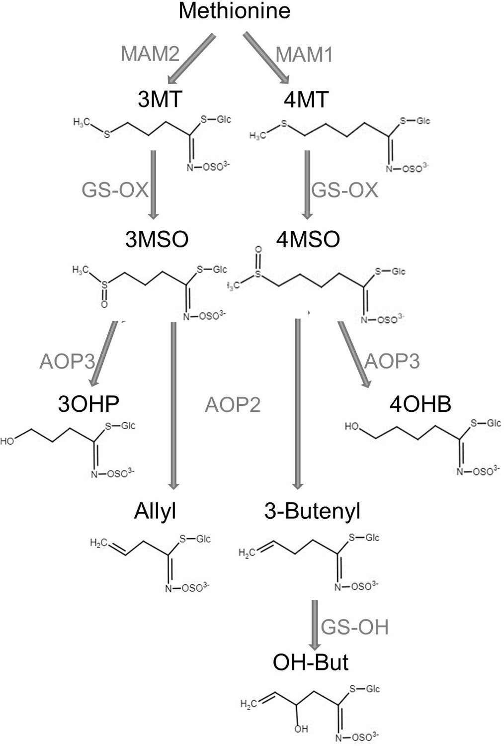
Aliphatic glucosinolate (GSL) biosynthesis pathway.
Short names and structures of the GSLs are in black. Genes encoding the causal enzyme for each reaction (arrow) are in gray. GS-OX is a gene family of five or more genes. OH-But: 2-OH-3-Butenyl.
Figure 3 with 3 supplements
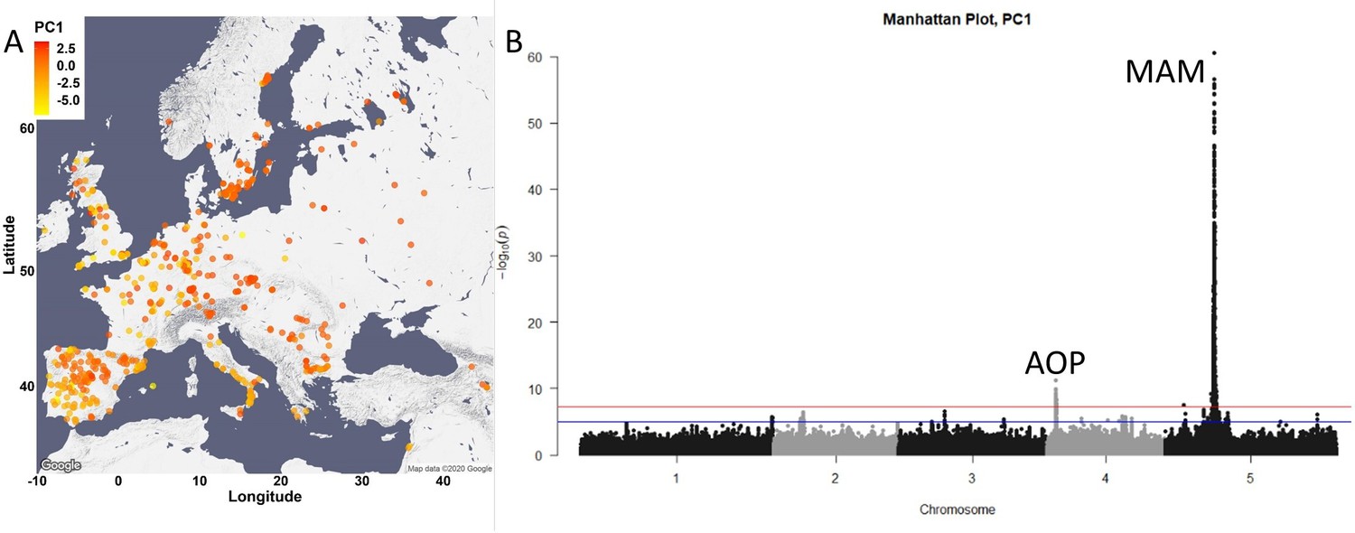
Glucosinolate variation across Europe is dominated by two loci.
(A) The accessions are plotted on the map based on their collection site and colored based on their principal component (PC)1 score. (B) Manhattan plot of genome-wideassociation analyses using PC1. Horizontal lines represent 5% significance thresholds using Bonferroni (red) and Benjamini–Hochberg (blue).
Figure 3—figure supplement 1
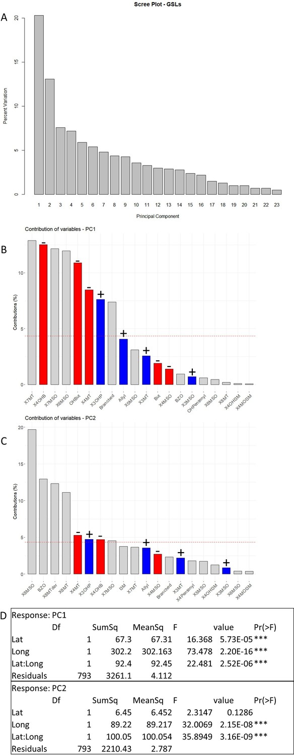
Glucosinolate (GSL)-based principal component (PC) analysis.
(A) Percentage of variance explained by each PC. (B, C) Contribution of the individual GSLs to PC1 (B) and PC2 (C). Red bars: contribution of four carbon GSLs; blue bars: contribution of three carbons GSLs. ± above the bar indicates if the contribution of the variable is positive or negative. (D) Linear model for PC1 and PC2 scores with the geographic parameters. Lat: latitude; Long: longitude.
Figure 3—figure supplement 2
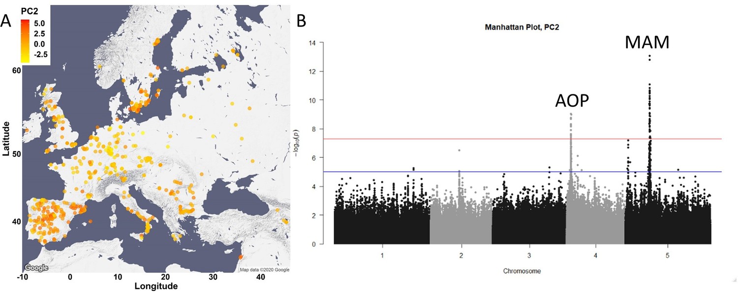
Glucosinolate variation across Europe is dominated by two loci.
(A) The accessions were plotted on the map based on their collection site and colored based on their principal component (PC)2 score. (B) Manhattan plot of genome-wideassociation analyses using PC2. Horizontal lines represent 5% significance thresholds using Bonferroni (red) and Benjamini–Hochberg (blue).
Figure 3—figure supplement 3
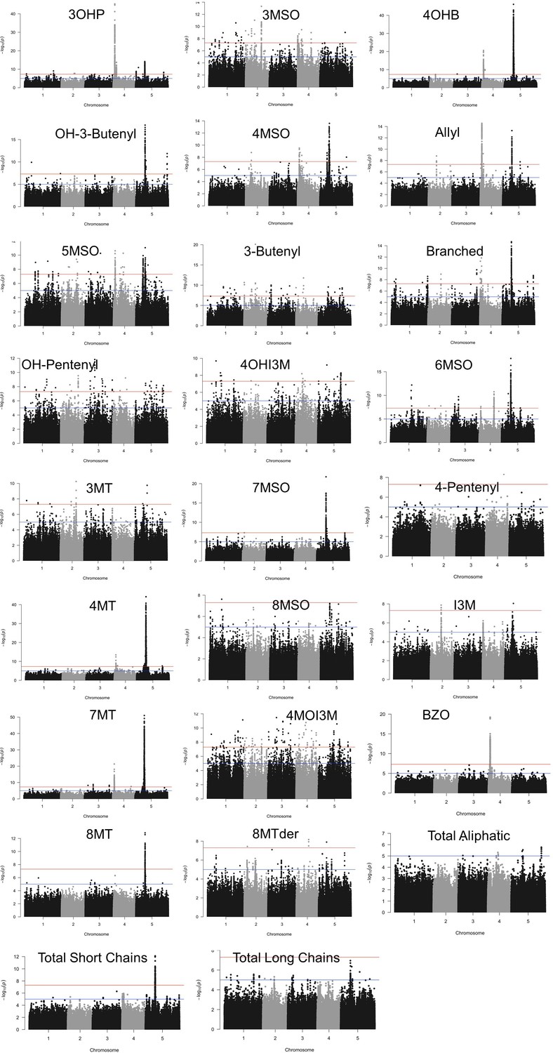
Manhattan plots of genome-wideassociation performed based on individual glucosinolate amounts as traits.
Horizontal lines represent 5% significance thresholds using Bonferroni (red) and Benjamini–Hochberg (blue).
Figure 4 with 4 supplements

Phenotypic classification based on glucosinolate (GSL) content.
(A) Using the GSL accumulation, each accession was classified to one of seven aliphatic short-chained GSL chemotypes based on the enzyme functions as follows: MAM2, AOP null: classified as 3MSO dominant, colored in yellow. MAM1, AOP null: classified as 4MSO dominant, colored in pink. MAM2, AOP3: classified as 3OHP dominant, colored in green. MAM1, AOP3: classified as 4OHB dominant, colored in light blue. MAM2, AOP2: classified as Allyl dominant, colored in blue. MAM1, AOP2, GS-OH non-functional: classified as 3-Butenyl dominant, colored in black. MAM1, AOP2, GS-OH functional: classified as 2-OH-3-Butenyl dominant, colored in red. The accessions were plotted on a map based on their collection sites and colored based on their dominant chemotype. (B) The coloring scheme with functional GSL enzymes in the aliphatic GSL pathway is shown with the percentage of accessions in each chemotypes (out of the total 797 accessions) shown in each box.
-
Figure 4—source data 1
Environmental conditions differentially associate with MAM status in the north versus the south.
Linear model for MAM status (carbon side chain length) was conducted with the indicated environmental parameters, for the northern and southern collection, separately (for more details, see Methods). The tables show p values for each term from the linear model. For the interaction with geography, the linear model was run using the total dataset, and the geography parameter (north or south) was added to the model.
- https://cdn.elifesciences.org/articles/67784/elife-67784-fig4-data1-v2.pptx
Figure 4—figure supplement 1
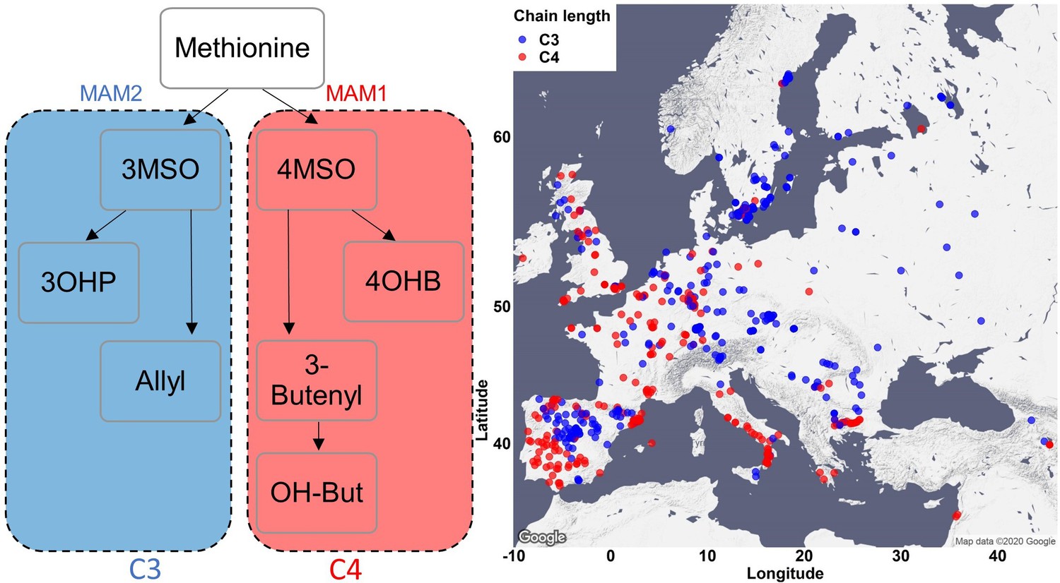
Phenotypic classification based on the dominant MAM enzyme.
Accessions were classified based on the side chain length of the aliphatic short-chained glucosinolates (GSLs). Accessions with a majority of GSLs containing three carbons in their side chains are classified as MAM2 dominant and colored in blue. Accessions with the majority of aliphatic short-chained GSLs containing four carbons in their side chains are classified as MAM1 dominant and colored in red. The accessions were plotted on a map based on their original collection sites.
Figure 4—figure supplement 2
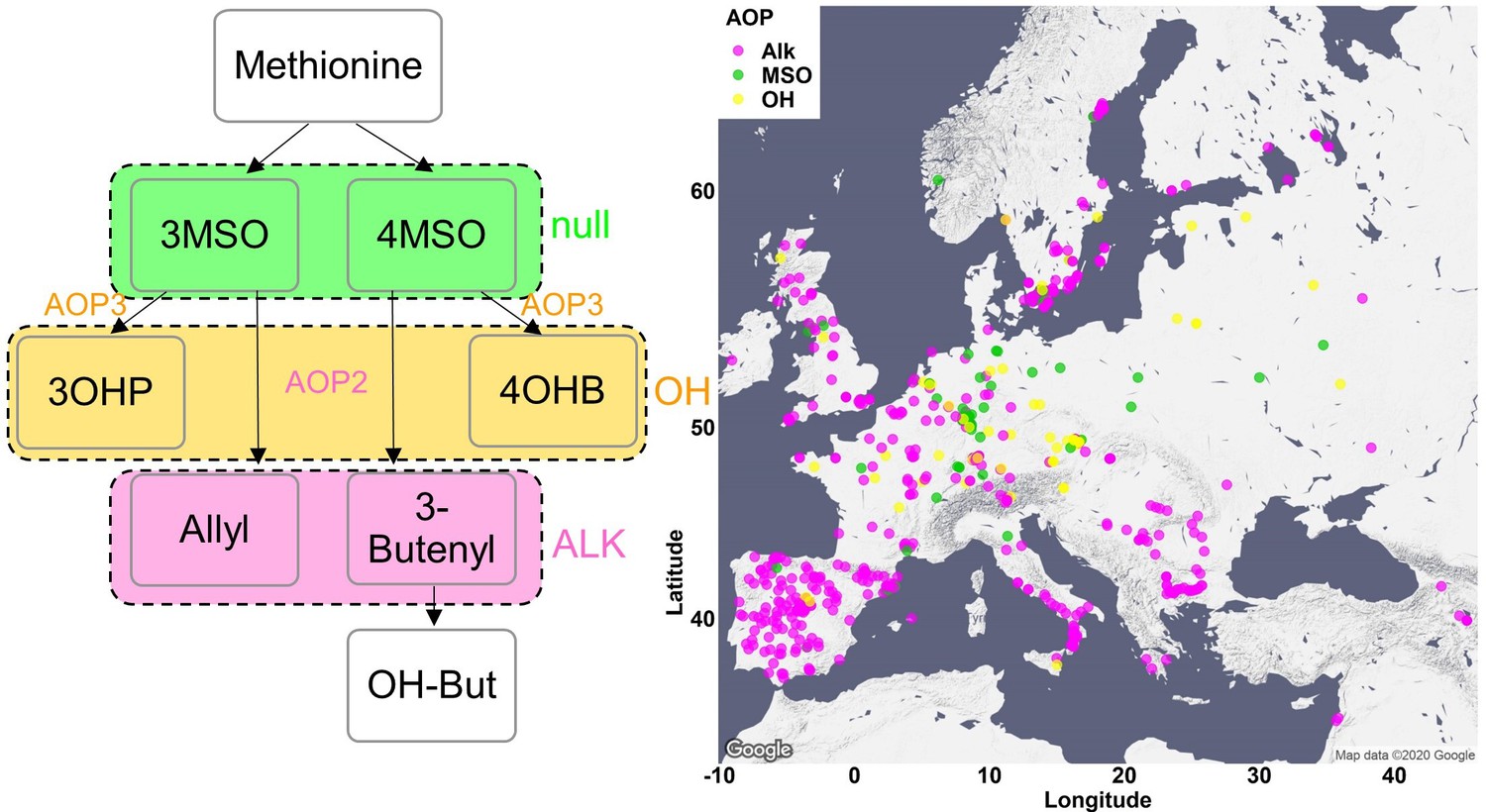
Phenotypic classification based on the dominant AOP enzymes.
Relative amounts of alkenyl glucosinolates (GSLs), alkyl GSLs and methylsulfinyl (MSO) GSLs were calculated in respect to the total short-chained aliphatic GSLs as described in the Methods section. Accessions with high amounts of alkenyl GSLs were classified as AOP2 dominant and colored in pink. Accessions with high amounts of alkyl GSLs were classified as AOP3 dominant and colored in orange. Accessions with high amounts of MSO GSLs were classified as AOP null and colored in green. The accessions were plotted on a map based on their original collection sites.
Figure 4—figure supplement 3

Phenotypic classification based on GS-OH enzyme activity.
The ratio between 2-OH-3-Butenyl to 3-Butenyl glucosinolate (GSL) was calculated only for MAM1-dominant accessions (accessions with GSLs containing four carbons in their side chain). Accessions with high amounts of 2-OH-3-Butenyl were classified as GS-OH functional and colored in black. Accessions with mostly 3-Butenyl were classified as GS-OH non-functional and colored in brown. The accessions were plotted on a map based on their original collection sites.
Figure 4—figure supplement 4
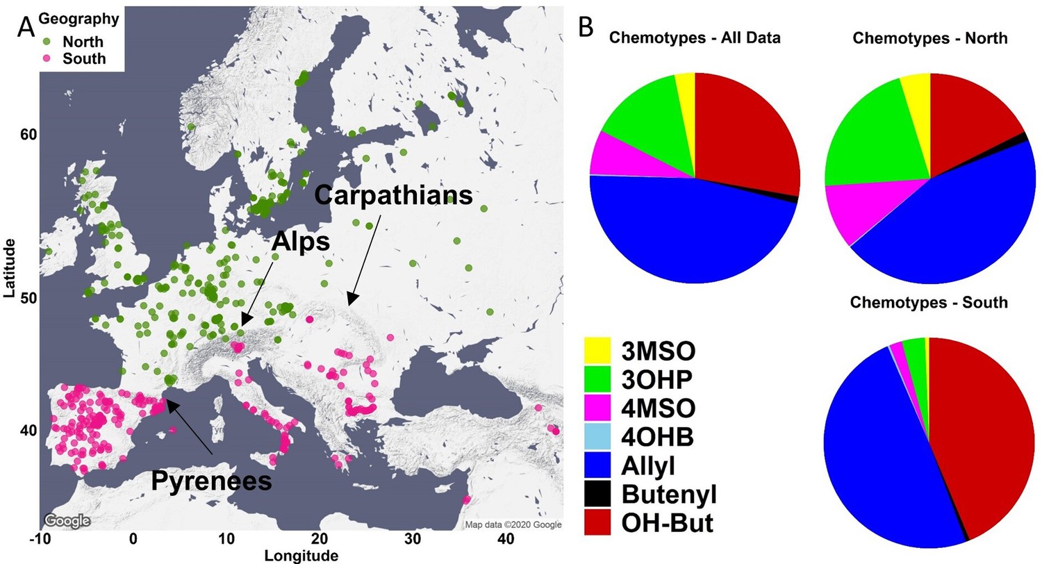
Geographic partitioning of the collection.
(A) The accessions were divided to two collections using the following chain of mountains: the Pyrenees between Spain and France, the Alps between Italy and Germany, and the Carpathians in the Balkan. The accessions that are located north of these mountains are referred to as the northern accessions and colored in green. The accessions located south of these mountains are referred to as the southern accessions and colored in pink. (B) The percentage of each chemotype was independently calculated in the south and north. Butenyl: 3-Butenyl; OH-But: 2-OH-3-Butenyl.
Figure 5 with 5 supplements
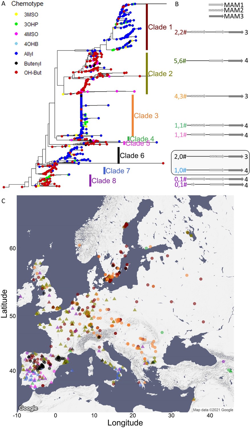
MAM3 phylogeny.
(A) MAM3 phylogeny of Arabidopsis thaliana accessions, rooted by Arabidopsis lyrata MAMb, which is not shown because of distance. Tree tips are colored based on the accession chemotype. (B) The genomic structure of the GS-Elong regions in the previously sequenced accessions is shown based on Kroymann et al., 2003. The structures in the box are based on sequences obtained in this work. The numbers left to the structures indicate the number of sequenced accessions in this work (left) or by Kroymann et al., 2003 (right). The numbers are colored based on their clades. Bright gray arrows represent MAM1 sequences, and dashed arrows represent MAM2 sequences. Dark gray arrows represent MAM3 sequences. The number to the right of the genomic cartoon represents the number of carbons in the side chain. (C) Collection sites of the accessions colored by their clade classification (from section A) and shaped based on the side chain length of the aliphatic short-chained glucosinolates (circles for C3, triangles for C4).
Figure 5—figure supplement 1

Support for the MAM3 tree clades classification.
(A) MAM3 phylogeny of 637 Arabidopsis thaliana accessions, rooted by Arabidopsis lyrata MAMb, excluding accessions with low-quality sequences. (B–E) MAM3 phylogeny of different combinations of A. thaliana accessions that were randomly chosen, rooted by A. lyrata MAMb. Bootstrap values >60 are indicated. In these trees, clade 2 was divided to two sub-clades. Clade’s MAM classification: clade 1, MAM2; clade 2, MAM1; clade 3, MAM2; clade 4, MAM1; clade 5, MAM1; clade 6, MAM2; clade 7, MAM1; clade 8, MAM1. (F) MYB37 phylogeny of A. thaliana accessions, rooted by the A. lyrate’s homologue (Al_scaffold_0006_2171, on chromosome 6), which is not shown because of distance. Tree tips are colored based on MAM3 clade’s classification as indicated in Figure 5A.
Figure 5—figure supplement 2

Genomic structure of the GS-Elong regions.
The GS-Elong locus from different accessions was sequenced, and the MAM1 and MAM2 structures were analyzed. The table indicates the dominant chemotype of each accession, the MAM status of each accession, and the number of accessions with the same structure that were sequences in this work. (A) Clade 1. (B) Clade 2. (C) Clade 3. (D) Clade 4. (E) Clade 5. (F) Clade 6. (G) Clade 7. T-1: truncated MAM1 (contains ~66% of 3’ MAM1). *2/1: chimeric version that contain ~50% of 5’ MAM2 and ~50% 3’ MAM1. ** 2/1: chimeric version that contain ~20% of 5’ MAM2 and ~80% 3’ MAM1.
-
Figure 5—figure supplement 2—source data 1
Sequences of MAM locus.
Sequencing for the accessions in Figure 5—figure supplement 2 were generated. The extracted regions are 30000bps upstream of AT5G23000 (MYB37) and 60000 bps downstream of AT5G23020 (MAM3).
- https://cdn.elifesciences.org/articles/67784/elife-67784-fig2-data2-v2.zip
Figure 5—figure supplement 3
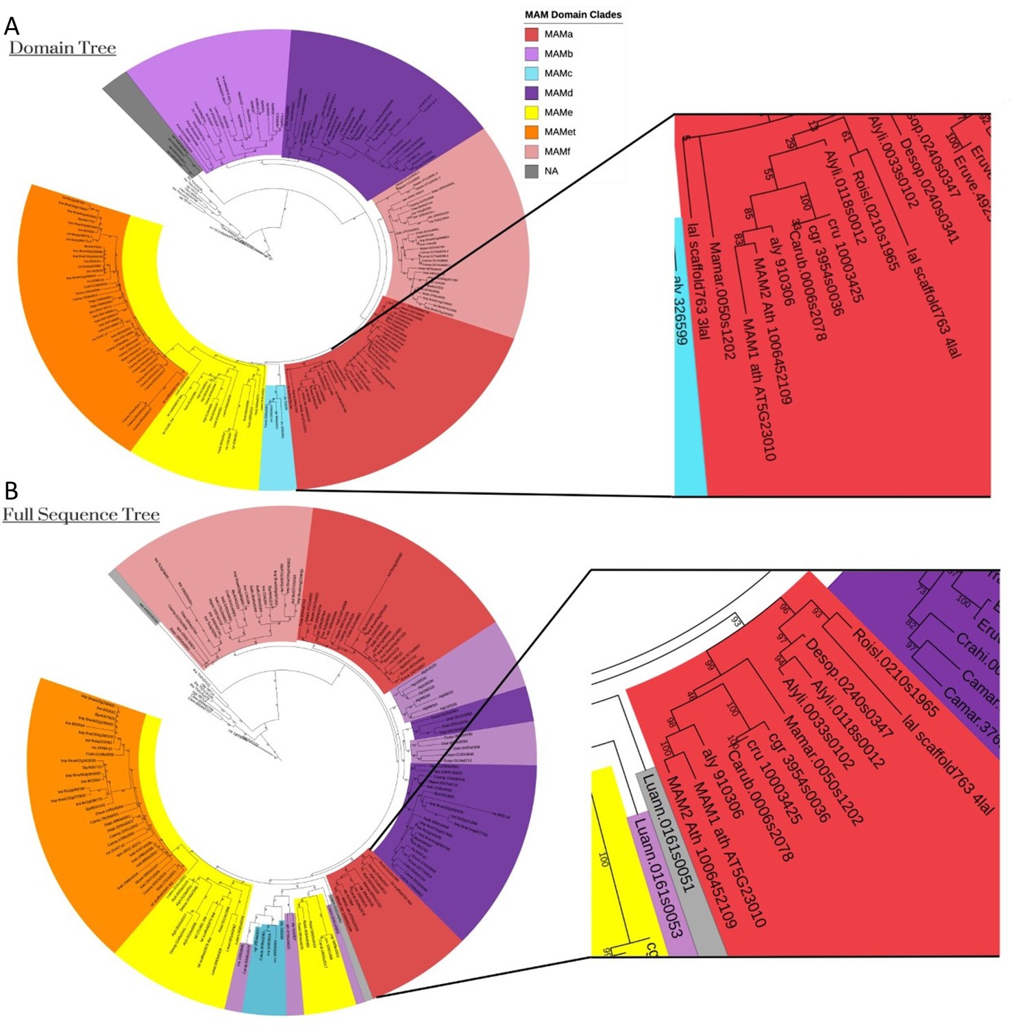
MAM2 is an Arabidopsis thaliana specific gene.
Domain (A) and full sequence (B) amino acid phylogenies of the MAM/IPMS gene family. Sequences were taken from Abrahams et al., 2020, which uses Arabidopsis thalina Col-0 genome and the MAM2 amino acid sequence 1006452109 from the Arabidopsis Information Resource (TAIR) database. Both MAM1 and MAM2 fall within the MAMa domain clade. MAM1 and MAM2 are sister to each other in either tree, with the next closest MAM gene belonging to Arabidopsis lyrata. These results support a recent duplication event specific to Arabidopsis thaliana and subsequent divergence and specialization.
Figure 5—figure supplement 4
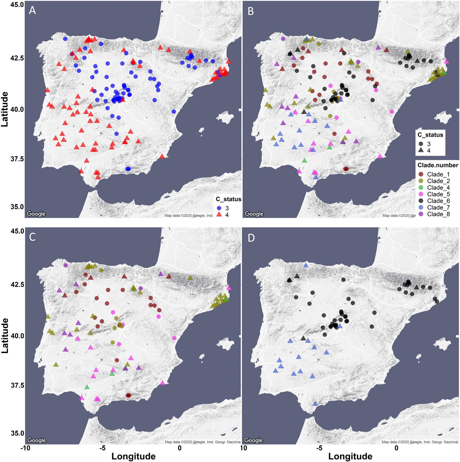
Iberia Peninsula presents low phenotypic variability and high genetic variation.
(A) All accessions from Iberia were plotted, colored and shaped based on the side chain length of the aliphatic short chained GSLs. Accessions with a majority of GSLs containing 3 carbons in their side chains are classified as MAM2 dominant, colored in blue and indicated as circles. Accessions with the majority of aliphatic short chained GSLs containing 4 carbons in their side chains are classified as MAM1 dominant, colored in red and indicated as triangles. (B) All accessions from Iberia were plotted, colored based on their MAM3 clade classification, and shaped based on the side chain length. (C) All accessions from Iberia except clades 6 and 7 were plotted, colored based on their MAM3 clade classification, and shaped based on the side chain length. (D) Clades 6 and 7 from Iberia were plotted, colored based on their MAM3 clade classification, and shaped based on the side chain length.
Figure 5—figure supplement 5
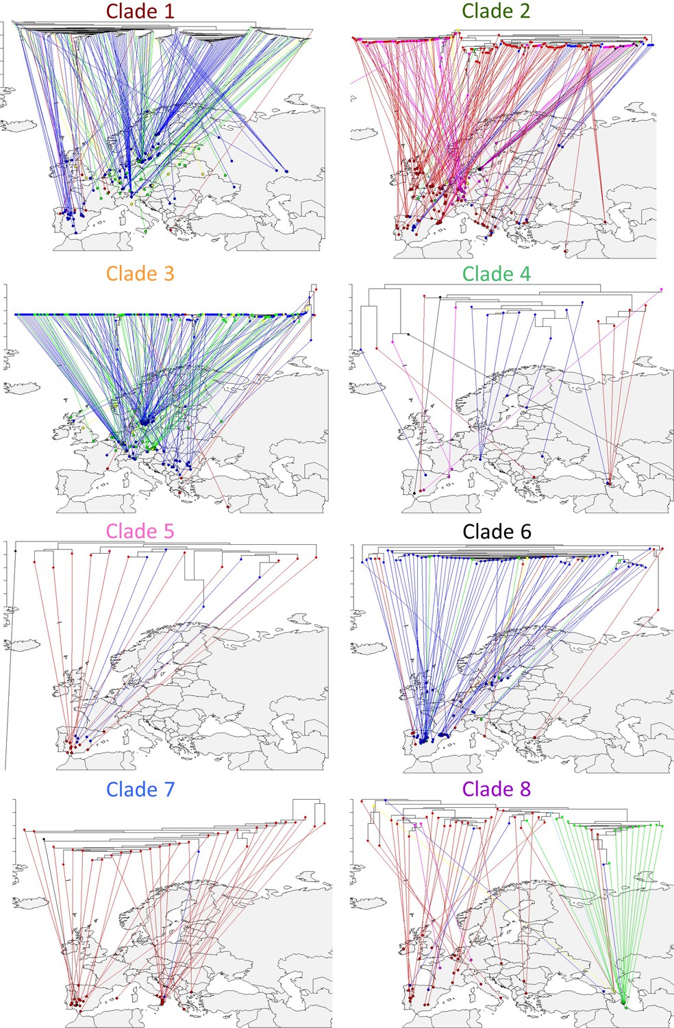
Geographic distribution of MAM haplotypes.
The MAM phylogeny is split by the major clades/haplotypes and each sub-clade’s phylogeny is reflected on the map. Tree tips are colored based on the accessions chemotype.
Figure 6 with 1 supplement
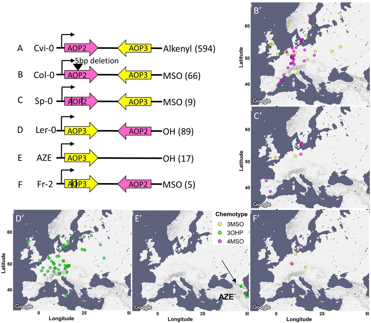
AOP genomic structure.
The genomic structure and causality of the major AOP2/AOP3 haplotypes are illustrated. Pink arrows show the AOP2 gene while yellow arrows represent AOP3. The black arrows represent the direction of transcription from the AOP2 promoter as defined in the Col-0 reference genome. Its position does not change in any of the regions. A-F represent the different structures. The black lines in C and F represent theoretical positions of independent variants creating premature stop codons. The GSL chemotype for each haplotype is listed to the right with the number of the accessions in brackets. The maps show the geographic distribution of the accessions from each structure.
Figure 6—figure supplement 1
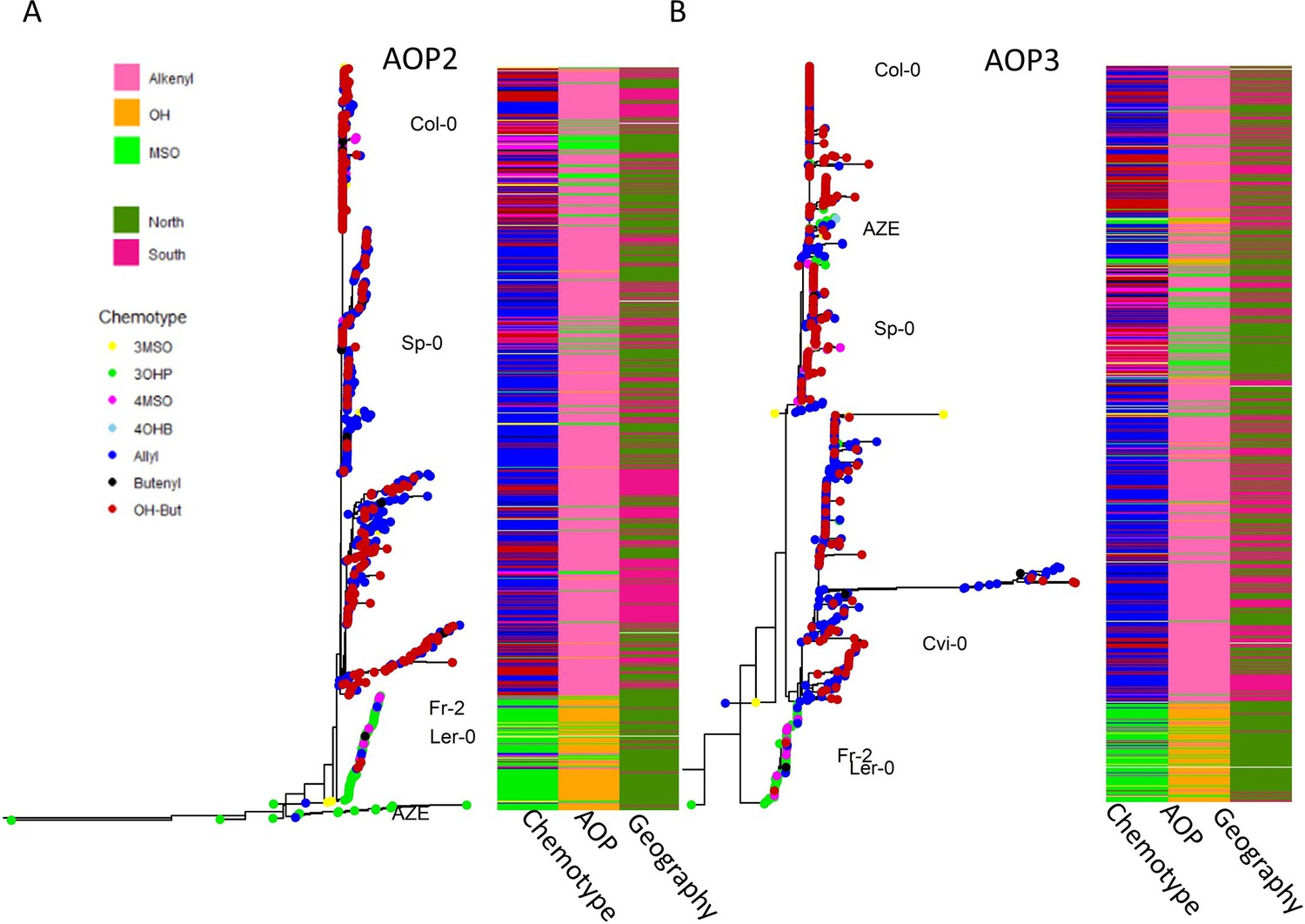
AOP phylogeny.
Separate phylogenies of AOP2 (A) and AOP3 (B) across Arabidopsis thaliana accessions. The trees are rooted by the matching gene in Arabidopsis lyrata, which is not shown because of distance. Tree tips are colored based on accessions’ chemotype. The first column of each heatmap represents the dominant chemotype’s identity. The second column of each heatmap represents the AOP functionality: pink for alkenyl (AOP2 dominant), orange for hydroxy (AOP3 dominant) and green for MSO (null). The third column represents the accessions’ geographic location: dark green for the north and dark pink for the south. The named accessions represent the haplotypes described in Figure 6.
Tables
Table 1
Environmental conditions differentially associate with major chemotypes across geographic location.
Linear model for the two major chemotypes, Allyl and 2-OH-3-Butenyl, was conducted with the indicated environmental parameters, for the northern and southern collection, separately (for more details, see Methods). The table shows p values for each term from the linear model. For the interaction with geography, the linear model was run using the total dataset, and the geography parameter (north or south) was added to the model.
| Environmental parameter | Effect on chemotype – north | Effect on chemotype – south | Interaction with geography |
|---|---|---|---|
| Genomic group | <0.0001 | <0.0001 | <0.0001 |
| Max temperature of warmest month | 0.0382 | <0.0001 | 0.3574 |
| Min temperature of coldest month | 0.0007 | <0.0001 | 0.0049 |
| Precipitation of wettest month | 0.1645 | 0.0003 | 0.0094 |
| Precipitation of driest month | 0.0665 | 0.2026 | 0.47425 |
| Distance to the coast | 0.2781 | 0.02680 | 0.1279 |
Table 2
GSOH structure.
The structures of GS-OH in the 3-Butenyl accessions are illustrated. Gray boxes represent exons, and blue lines represent introns. Black line represents a mutation, and gray lines represent unknown lesions in hypothetical locations. The above mutations create non-functional GS-OH alleles. The fractions of the mutated accessions were calculated out of the total number of 3-Butenyl and OH-3-Butenyl accessions. The observed frequencies were calculated as the ratio between number of accessions with the specific mutation in non-C4 Alkenyl accessions and all the non-C4 Alkenyl accessions, as mentioned in the parentheses.
| Accession | Type of mutation | Allele structure | Fraction (out of C4 Alkenyl accessions) | Observed frequency (out of non-C4 Alkenyl accessions) |
|---|---|---|---|---|
| Sorbo, Pien | Polymorphism at SNP10831302 |  | 0.009 (2/226) | 0.067 (38/564) |
| Cvi-0 | Active site mutation |  | 0.004 (1/226) | 0.025 (14/564) |
| IP-Mot-0, IP-Tri-0 | Gene deletion |  | 0.009 (2/226) | 0.055 (31/564) |
| Multiple accessions (T670, FlyA-3, Ting-1, T880, T710, T850) | Unidentified mutations |  | 0.026 (6/226) | Unknown |
Additional files
-
Supplementary file 1
GSLs data.
(A) List of GSLs and structures. (B) Accessions and glucosinolate (GSL) data – raw data. (C) Heritability values. (D) Accessions and GSL data – emmeans.
- https://cdn.elifesciences.org/articles/67784/elife-67784-supp1-v2.xlsx
-
Supplementary file 2
SNPs in glucosinolates (GSLs)-related loci under different genome-wide association (GWA) studies: GSL values were used as traits to conduct GWA studies.
The number of significant SNPs in the GSLs related loci (columns c to o) was counted for each GWA study separately. Rows 2–3: common name and AT number of gene/s in the loci. Rows 4–5: upstream and downstream positions of the relevant loci (10 kb were added upstream and downstream of the genes). Rows 6–33: GSLs traits used for GWA studies. In black: number of SNPs with p value between 0.00001 and 0.0000001. In red: number of SNPs with p value equal or smaller than 0.0000001.
- https://cdn.elifesciences.org/articles/67784/elife-67784-supp2-v2.xlsx
-
Transparent reporting form
- https://cdn.elifesciences.org/articles/67784/elife-67784-transrepform1-v2.docx
Download links
A two-part list of links to download the article, or parts of the article, in various formats.
Downloads (link to download the article as PDF)
Open citations (links to open the citations from this article in various online reference manager services)
Cite this article (links to download the citations from this article in formats compatible with various reference manager tools)
Genetic variation, environment and demography intersect to shape Arabidopsis defense metabolite variation across Europe
eLife 10:e67784.
https://doi.org/10.7554/eLife.67784


