Distinct synaptic transfer functions in same-type photoreceptors
- Institute for Ophthalmic Research, University of Tübingen, Germany
- Center for Integrative Neuroscience, University of Tübingen, Germany
- Bernstein Center for Computational Neuroscience,Centre for Integrative Neuroscience, all: University of Tubingen, Germany
- School of Life Sciences,University of Sussex, United Kingdom
Figures
Figure 1 with 1 supplement
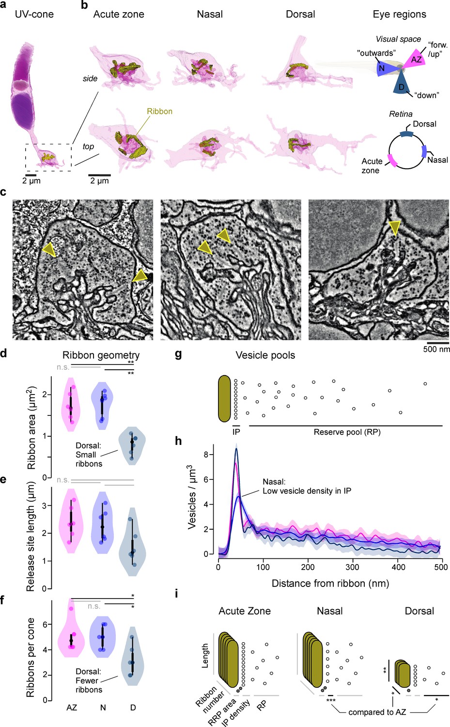
Eye-region-specific structural tuning of a ribbon synapse in UV-cones.
(a) Example of a full UV-cone reconstruction, taken from the acute zone. Dark purple: nucleus; light purple: mitochondria; purple: outer segment; yellow: ribbon. (b) Zoom-ins of UV-cone terminals from different regions, which are illustrated on the rightmost panels. Ribbons are highlighted in yellow. Each terminal is shown from the side (top) and from below (bottom). (c) Example electron microscopy images from each zone, with arrowheads indicating ribbons. (d–f) Violin plots of the ribbon geometry and number for the three different regions (two-sided shuffling test with Bonferroni correction, nAZ, nN, nD = 6, 6, 6, *p<0.05, **p<0.01). (g) Two-dimensional schema of the vesicle pools at a ribbon synapse. (h) Mean and 95% confidence intervals for vesicle densities as a function of distance to the ribbon. Predictions are made from a generalised additive model (GAM, Materials and methods; see Figure 1—figure supplement 1 for statistical comparisons). (i) Summary schema of observed Electron microscopic-level differences between UV-cones at the level of ribbon geometry, number, and vesicle distributions. Asterisks indicate significant differences compared to acute zone (AZ). The stacked ribbons (gold) indicate the ribbon number per cone, whereas the vesicles (small circles) are exemplified in a two-dimensional plane for a single ribbon.
Figure 1—figure supplement 1
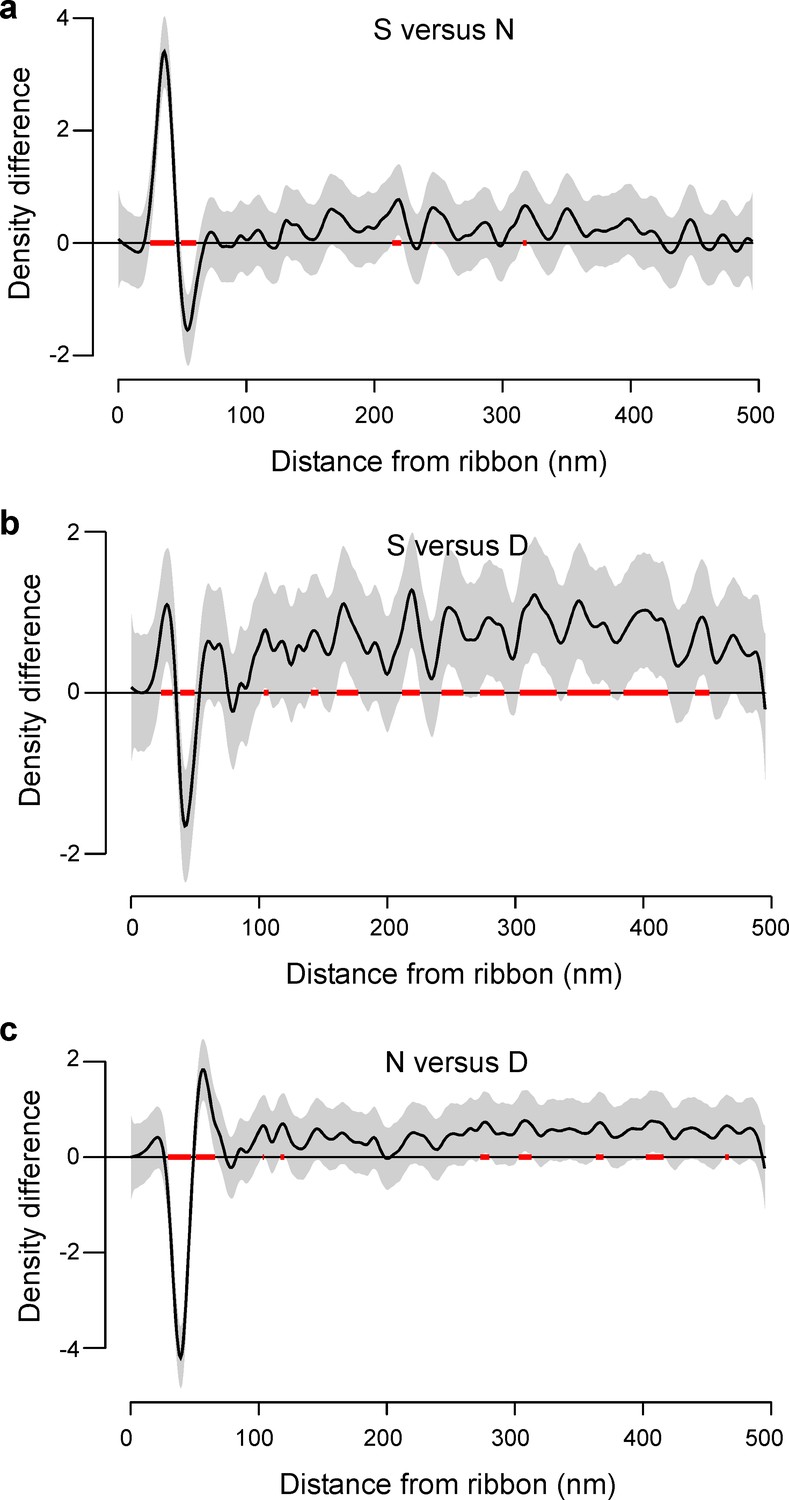
Statistical comparison of spatial vesicle distributions.
(a-c) Pairwise comparison of the three regions, modelled as generalised additive model (Materials and methods). The estimated mean difference (black) and 95% confidence intervals (grey) are shown and distances with significant differences (α = 0.05) are highlighted (red).
Figure 2 with 1 supplement
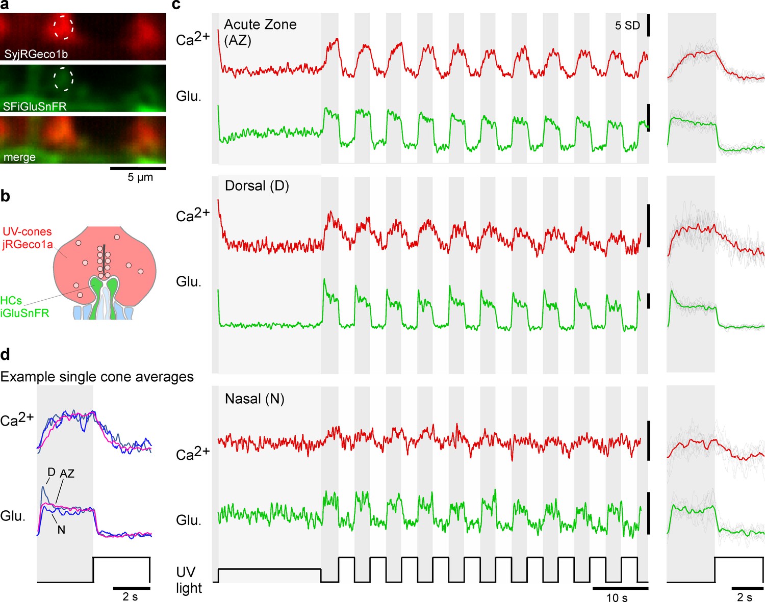
Simultaneous in vivo imaging of synaptic calcium and release.
(a, b) Simultaneously acquired two-photon scans of cone terminals and opposing horizontal cell dendrites, with cone pedicles expressing SyjRGeco1b (red), and horizontal cell dendrites expressing SFiGluSnFR (green), and schematic representation, showing the cone pedicle (red) with ribbon and vesicles, as well as horizontal cell processes (green) and bipolar cell dendrites (blue). (c) Examples of raw calcium (red) and glutamate (green) traces recorded simultaneously from single UV-cones, one from each eye region as indicated. The averaged traces and superimposed stimulus repetitions are shown on the right. (d) Overlay of the averaged traces in (c), highlighting different glutamate responses despite very similar calcium responses.
Figure 2—figure supplement 1
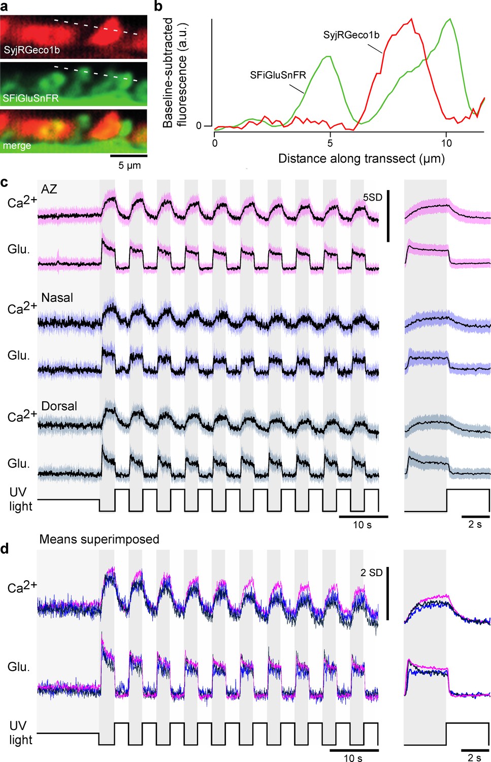
Mean calcium and glutamate traces per region.
(a) As Figure 2a, example ‘red’ (top) and ‘green’ (middle) fluorescence channels acquired simultaneously, and merged (bottom) and (b) extracted fluorescence profiles in the two channels as indicated. Note the absence of any obvious ‘bleed-through’, indicating good spectral separation of the two fluorescence detection bands. (c) Z-scored recordings before scaling and denoising (mean ± SD). (d) Superimposed means of the data shown in (c).
Figure 3 with 1 supplement
Physiological differences in light responses between UV-cones from different eye regions.
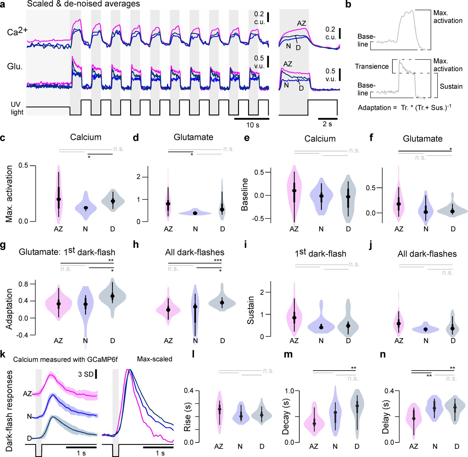
(a) Scaled and denoised calcium and glutamate recordings averaged across multiple regions of interest (ROIs) (Materials and methods). We refer to the scaling as calcium units (c.u.) and vesicle units (v.u.) as the same traces also serve as input for the biophysical model (see Figure 4). (b) Schema of the calculated indices in (c–j) (Materials and methods). The transience index is computed as max.-sustainmax. (c–j) Quantification of physiological differences for the three different retinal regions (two-sided shuffling test with Bonferroni correction, nAZ, nN, nD = 30, 9, 16, *p<0.05, **p<0.01, ***p<0.001). (k) GCaMP6f recordings from Yoshimatsu et al., 2020b. Mean ± SD and overlaid mean traces in response to a 200 ms dark flash stimulus. (l–n) Quantification of physiological differences for the GCaMP6f recordings: time constants for an exponential rise, decay, as well as delay time to response (see also Materials and methods) (two-sided shuffling test with Bonferroni correction, nAZ, nN, nD = 13, 17, 22, *p<0.05, **p< 0.01, ***p<0.001).
Figure 3—figure supplement 1
Preprocessing of calcium and glutamate recordings.
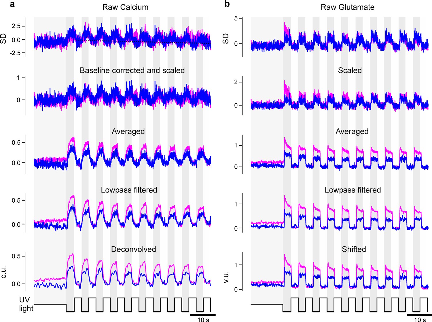
(a) The raw (z-scored) calcium data is first corrected for a linear decay of the baseline (dotted black line). It is then scaled such that the UV-bright intervals have mean 0 and standard deviation 1 (second row). After averaging all recordings of one zone (third row), the traces are then lowpass filtered and finally deconvolved (last row). We only included the acute zone (AZ) and nasal zone in this illustration. (b) As (a) but for the glutamate data, but no baseline correction and deconvolution was applied. As a final step, the glutamate traces were shifted to have only non-negative values (last row).
Figure 4 with 1 supplement

A model of calcium-evoked release from the ribbon.
(a) Schema of the movement of vesicles at a ribbon synapse. The vesicles move from the reserve pool (RP) to the intermediate pool (IP) at the ribbon and finally to the readily releasable pool (RRP) close to the membrane before they are released into the synaptic cleft to activate the dendrites of invaginating horizontal cells (HCs). (b) Schema of the parameter inference: over several rounds, samples are first drawn from a prior, the model is then evaluated and summary statistics on which the relevant loss function is calculated are extracted. Based on these values and the sampled parameters, a mixture of density network (MDN) is trained and evaluated to get the posterior/prior for the next round. (c) Model predictions for the three regions (mode and 90% prediction intervals from posterior samples in colour, data in black). (d) Mode and 90% prediction intervals of the model’s non-linearity. (e) Prior and one-dimensional marginals of the posterior distributions (see Figure 4—figure supplement 1a for the two-dimensional marginals). The units are vesicle units (v.u.) and calcium units (c.u.), referring to the scale invariance of the model. (f) Evaluation of the best region-specific models on its region-specific calcium traces. (g) Evaluation of best region-specific model on the calcium races of the other regions. (h) Evaluation of the linear baseline model (model in colour, data in black): especially the transient components are missed. See Figure 3—figure supplement 1b for a quantification of the goodness of fits.
Figure 4—figure supplement 1
Marginals of model posteriors, and comparison in model performance.
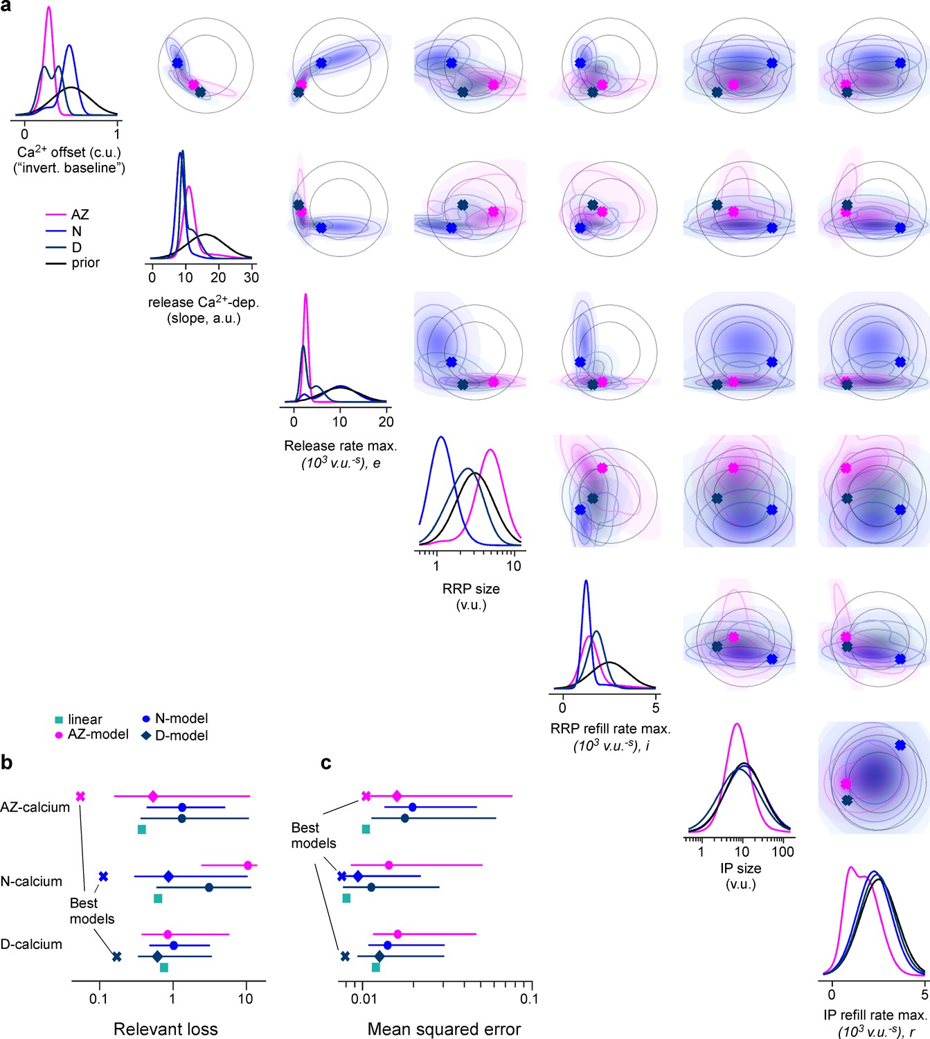
(a) One- and two-dimensional marginals of the posterior as well as of the prior. Best parameters per region are marked as a cross. (b) Median with 5th and 95th percentiles (error bars) for the relevant loss based on the summary statistics (Materials and methods), as well as the loss for the best zone-specific and the linear baseline model for comparison. (c) Same as (b) but loss as mean squared error (MSE) between glutamate recordings and model output.
Figure 5

Sobol Indices.
(a-c) Sensitivity of the model for the different model parameters measured by the Sobol index (Materials and methods). The Sobol index measures the expected reduction in relative variance for the fixation of parameter θi. It depends on the posterior distribution and is therefore different for the fits to the three regions.
Figure 6
General rules of ribbon tuning: basic response parameters.
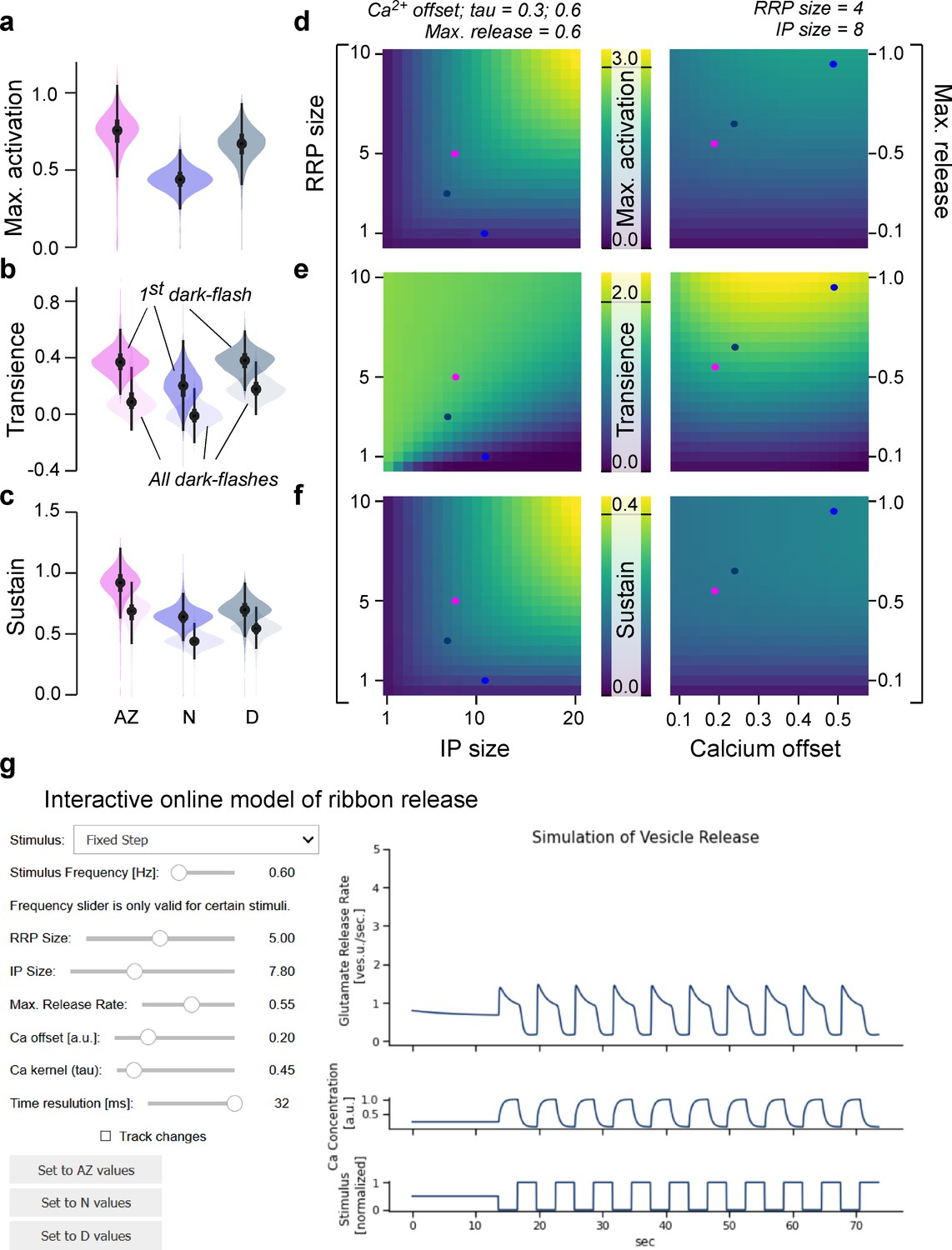
(a-c) The same indices as in Figure 3, but here calculated on 10,000 model evaluations on samples from the posteriors. The model has learned the differences between the retinal regions and reproduces these differences (see Figure 3 for comparison). (d-f) Indices as in (a–c), calculated on different parameter combinations as indicated. For this analysis, a step-stimulus feeding into a linear calcium model was added as the input to the release model (Materials and methods). For definition of the indices, see also Figure 3b. (g) Screenshot of the interactive online model, available at http://www.tinyurl.com/h3avl1ga.
Figure 7
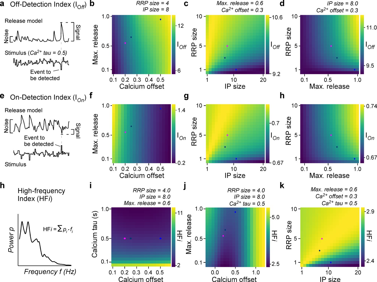
General rules of ribbon tuning: event detection and high-frequency encoding.
(a) An off-detection index (IOff) measures the model’s baseline noise-normalised response amplitude to an off-event in the stimulus as indicated (Materials and methods). (b–d) IOff for different parameter combinations. (e–h) As (a–d), but for an on-detection index (IOn). (h) The high-frequency index (HFi) is a weighted sum of the discretised power spectrum and indicates the behaviour in a high-frequency regime. (i–k) HFi for different parameter combinations. The fixed parameters are shown as titles in each panel. Note the different colour scales between panels. Further note that in (j) we explored the x0 parameter space up to extreme response behaviour, which may not be physiologically plausible.
Additional files
Download links
A two-part list of links to download the article, or parts of the article, in various formats.
Downloads (link to download the article as PDF)
Open citations (links to open the citations from this article in various online reference manager services)
Cite this article (links to download the citations from this article in formats compatible with various reference manager tools)
Distinct synaptic transfer functions in same-type photoreceptors
eLife 10:e67851.
https://doi.org/10.7554/eLife.67851


