Low-dimensional learned feature spaces quantify individual and group differences in vocal repertoires
- Department of Computer Science, Duke University, United States
- Center for Cognitive Neurobiology, Duke University, United States
- Department of Neurobiology, Duke University, United States
- Department of Biostatistics & Bioinformatics, Duke University, United States
- Department of Electrical and Computer Engineering, Duke University, United States
Figures
Figure 1 with 1 supplement

Variational autoencoders (VAEs) learn a latent acoustic feature space.
(a) The VAE takes spectrograms as input (left column), maps them via a probabilistic ‘encoder’ to a vector of latent dimensions (middle column), and reconstructs a spectrogram via a ‘decoder’ (right column). The VAE attempts to ensure that these probabilistic maps match the original and reconstructed spectrograms as closely as possible. (b) The resulting latent vectors can then be visualized via dimensionality reduction techniques like principal components analysis. (c) Interpolations in latent space correspond to smooth syllable changes in spectrogram space. A series of points (dots) along a straight line in the inferred latent space is mapped, via the decoder, to a series of smoothly changing spectrograms (right). This correspondence between inferred features and realistic dimensions of variation is often observed when VAEs are applied to data like natural images (Kingma and Welling, 2013; Rezende et al., 2014).
Figure 1—figure supplement 1
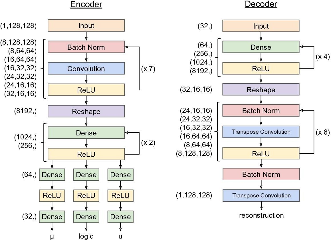
Variational autoencoder network architecture.
The architecture outlined above was used for all training runs. The looping arrows at the right of the encoder and decoder denote repeated sequences of layer types, not recurrent connections. For training details, see Materials and methods. For implementation details, see https://github.com/pearsonlab/autoencoded-vocal-analysis (Goffinet, 2021; copy archived at swh:1:rev:f512adcae3f4c5795558e2131e54c36daf23b904).
Figure 2 with 6 supplements
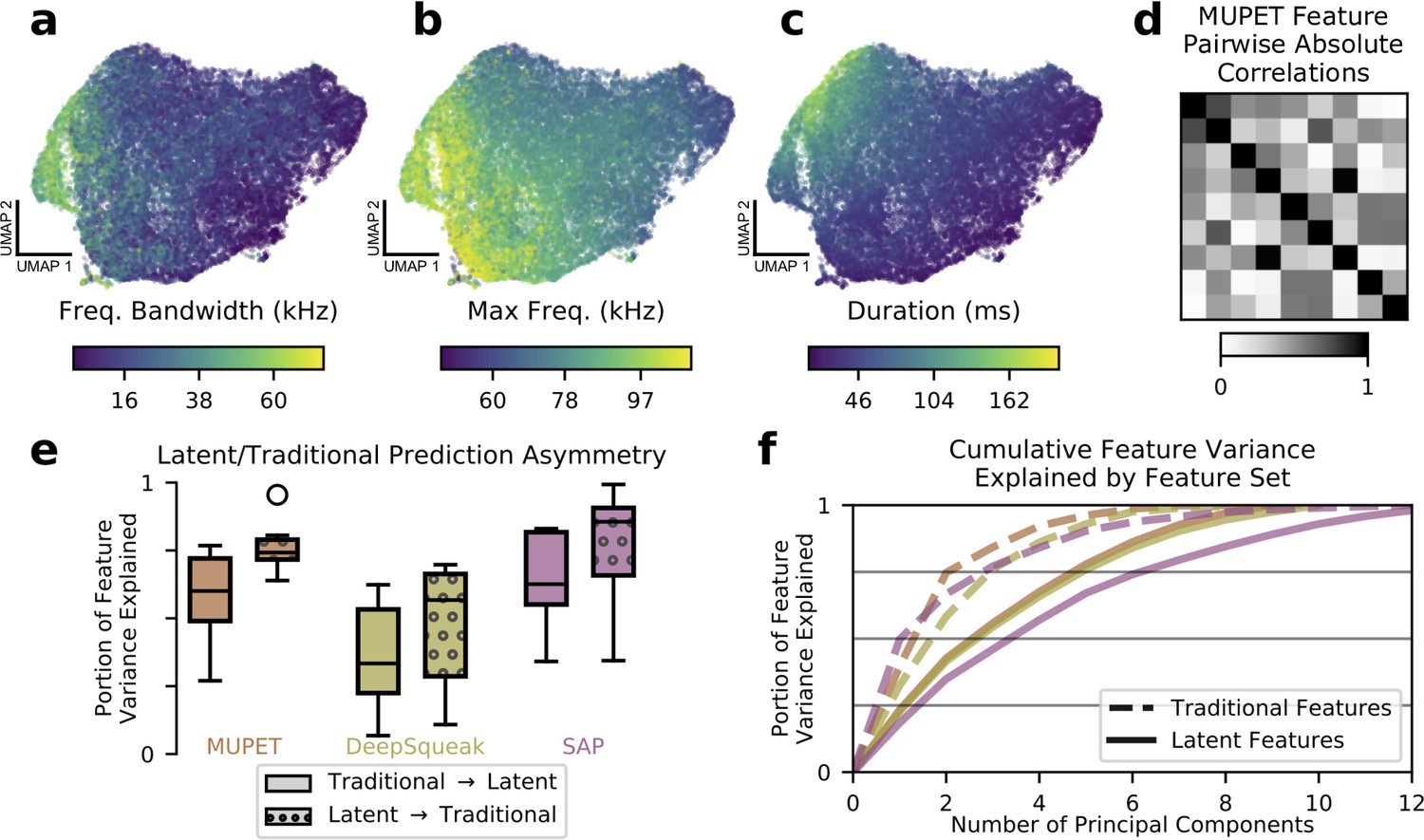
Learned acoustic features capture and expand upon traditional features.
(a–c) UMAP projections of latent descriptions of mouse ultrasonic vocalizations (USVs) colored by three traditional acoustic features. The smoothly varying colors show that these traditional acoustic features are represented by gradients within the latent feature space. (d) Many traditional features are highly correlated. When applied to the mouse USVs from (a) to (c), the acoustic features compiled by the analysis program MUPET have high correlations, effectively reducing the number of independent measurements made. (e) To better understand the representational capacity of traditional and latent acoustic features, we used each set of features to predict the other and vice versa (see Materials and methods). We find that, across software programs, the learned latent features were better able to predict the values of traditional features than vice versa, suggesting that they have a higher representational capacity. Central line indicates median, upper and lower box the 25th and 75th percentiles, respectively. Whiskers indicate 1.5 times the interquartile range. Feature vector dimensions: MUPET, 9; DeepSqueak, 10; SAP, 13; mouse latent, 7; zebra finch latent, 5. (f) As another test of representational capacity, we performed PCA on the feature vectors to determine the effective dimensionality of the space spanned by each set of features (see Materials and methods). We find in all cases that latent features require more principal components to account for the same portion of feature variance, evidence that latent features span a higher dimensional space than traditional features applied to the same datasets. Colors are as in (e). Latent features with colors labeled ‘MUPET’ and ‘DeepSqueak’ refer to the same set of latent features, truncated at different dimensions corresponding to the number of acoustic features measured by MUPET and DeepSqueak, respectively.
Figure 2—figure supplement 1
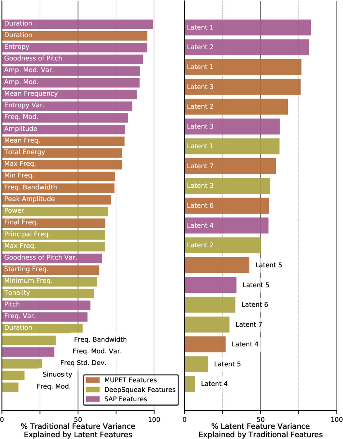
Variance explained by traditional and latent features.
Left column: named acoustic feature variance explained by latent features. Right column: latent acoustic feature variance explained by named acoustic features. Values reported are the results of k-nearest neighbor classification averaged over five shuffled test/train folds (see Materials and methods).
Figure 2—figure supplement 2
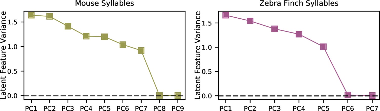
The variational autoencoder (VAE) learns a parsimonious set of acoustic features.
Figure 2—figure supplement 3
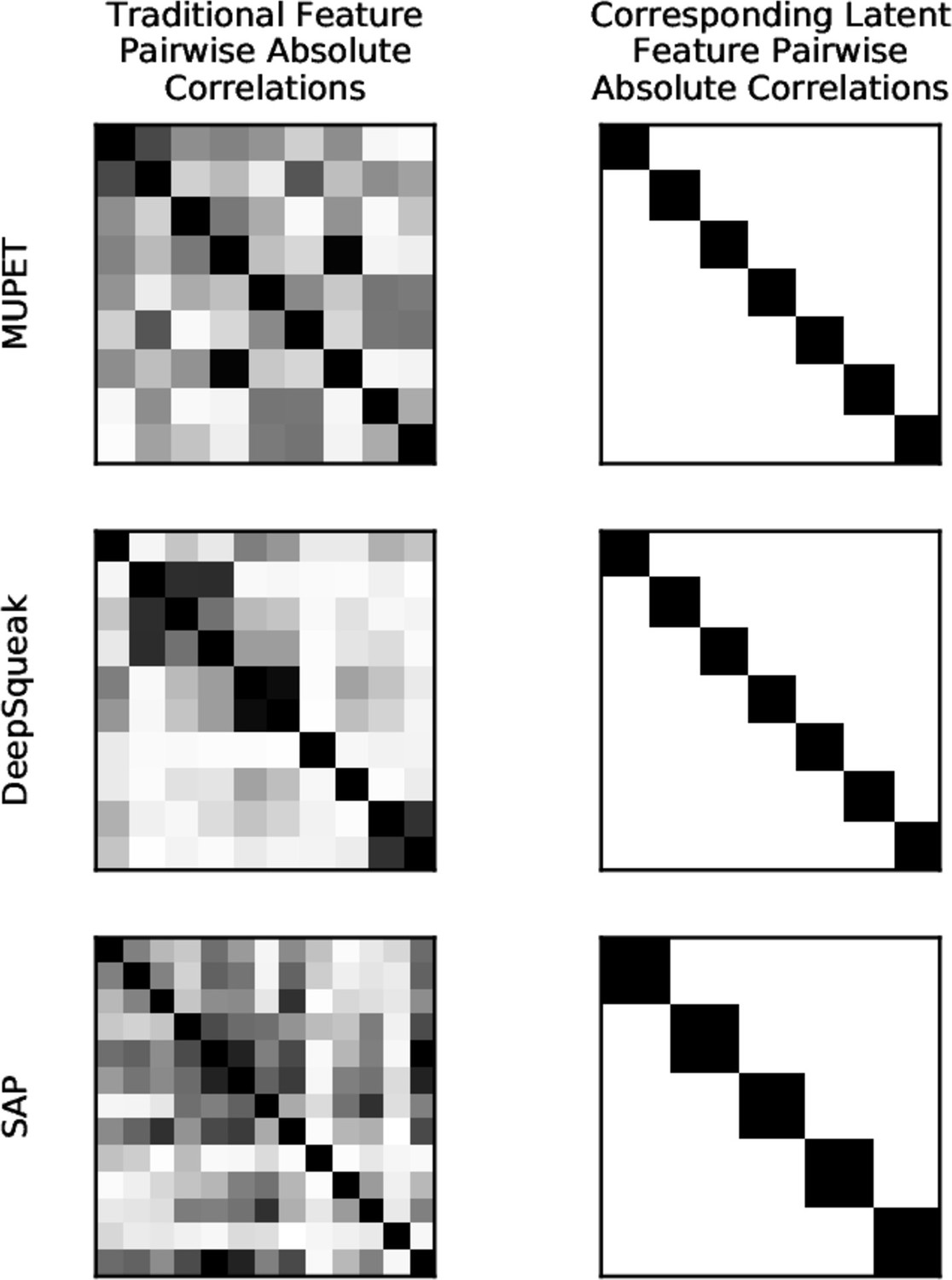
Correlations among traditional and latent features.
Traditional acoustic features are highly correlated. Left column: pairwise absolute correlations between named acoustic features when applied to the datasets in Figure 2. Right column: pairwise absolute correlations of latent features for the same datasets.
Figure 2—figure supplement 4
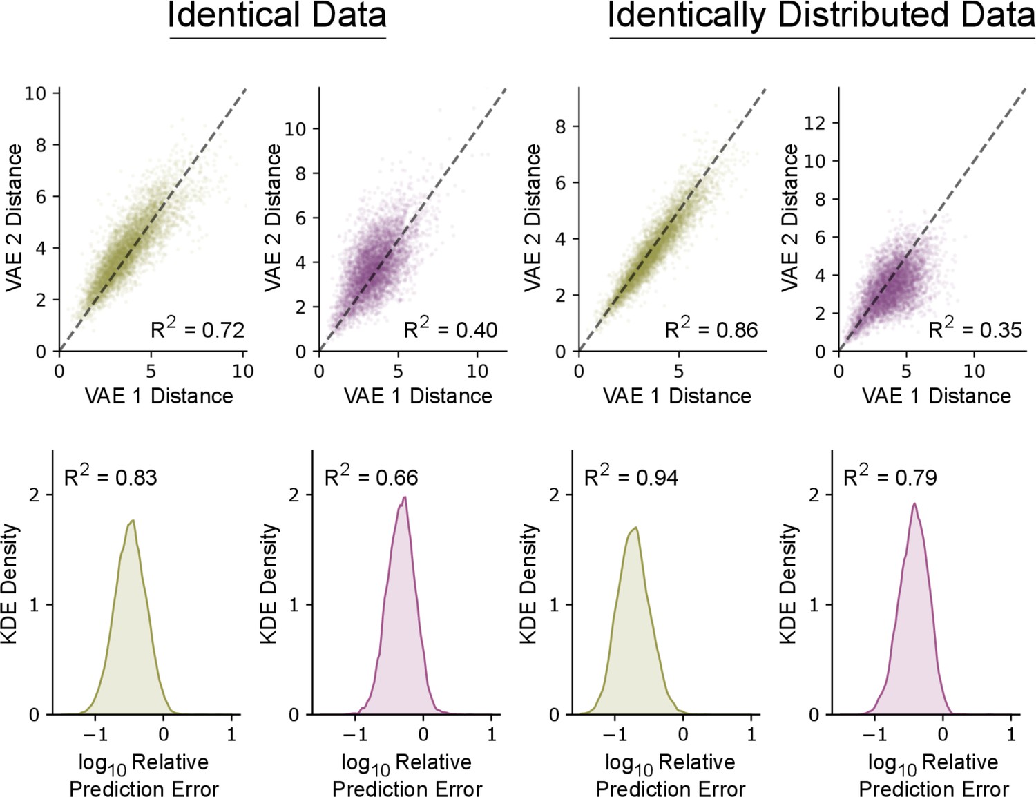
Reproducibility of variational autoencoder (VAE) latent features.
The VAE produces similar latent features when retraining on identical data and disjoint splits of the same dataset. Top row: pairwise latent distances of 5000 random pairs of syllables under separately trained VAEs. Bottom row: the distribution of errors when predicting the latent means of one VAE from the other using linear regression. Errors are normalized relative to the root-mean-square (RMS) distance from the mean in latent space so that -1 corresponds to 10% of the RMS distance from the mean. For predicting a multivariate Y from a multivariate X, we report a multivariate R2 value: . first column: Two VAEs are trained on the set of mouse syllables from Figure 2a-c. Second column: Two VAEs are trained on the set of zebra finch syllables from Figure 4a-c. Third column: Two VAEs are trained on two disjoint halves of the mouse syllables from Figure 2a-c. Fourth column: Two VAEs are trained on two disjoint halves of the zebra finch syllables from Figure 4a-c. Note that retraining produces less consistent results for zebra finch syllables, possibly because the relative orientations and positions of well-separated clusters is underdetermined by the data.
Figure 2—figure supplement 5
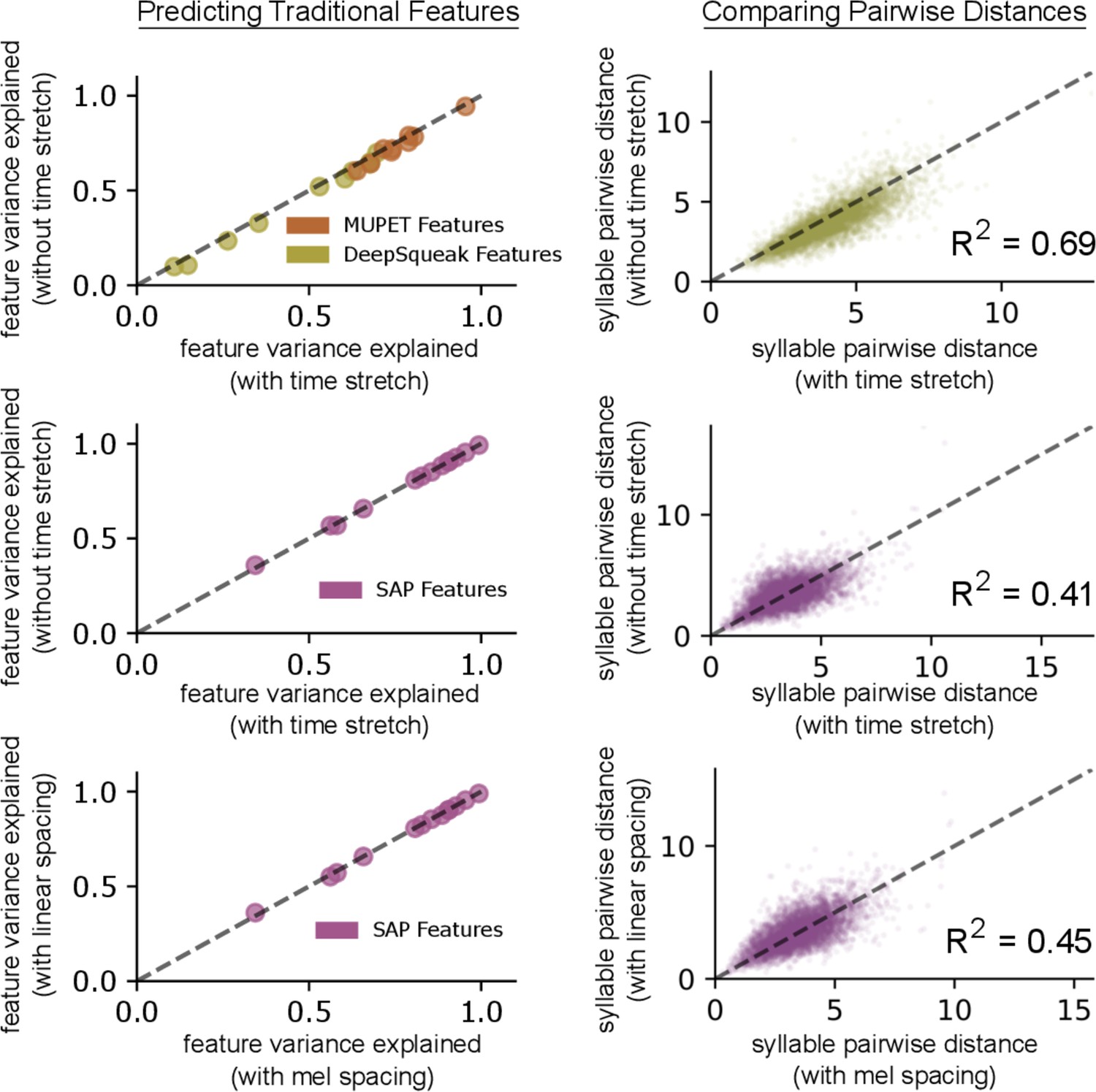
The effect of time stretch and frequency spacing parameters.
Top row: two variational autoencoder (VAEs) are trained on the mouse ultrasonic vocalization (USV) syllables from Figure 4d, one with time stretching to expand the spectrograms of short syllables (see Materials and methods) and one without. When using the learned latent features from each model to predict the values of acoustic features calculated by MUPET and DeepSqueak, we observe a small but consistent performance gain using time stretching (left column). Additionally, we find a good correspondence between pairwise Euclidean distances in the two learned feature spaces (right column), indicating the two latent spaces have similar geometries. Middle row: repeating the same comparison with zebra finch song syllables from Figure 4a-c, we find fairly consistent pairwise distances across the two latent spaces (right) and no substantial effect on the performance of predicting acoustic features calculated by SAP (left). Bottom row: two VAEs trained on the same zebra finch song syllables, one with linearly spaced spectrogram frequency bins and the other with mel-spaced frequency bins, have fairly consistent pairwise distances across the two latent spaces (right) and no substantial effect on the performance of predicting acoustic features calculated by SAP (left).
Figure 2—figure supplement 6
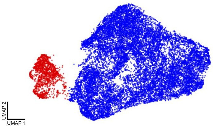
Removing noise from single mouse ultrasonic vocalization (USV) recordings (see Recordings).
Above is a UMAP projection of all detected USV syllables. The false positives (red) cluster fairly well, so they were removed from further analysis. Of the 17,400 total syllables detected, 15,712 (blue) remained after removing the noise cluster.
Figure 3 with 3 supplements
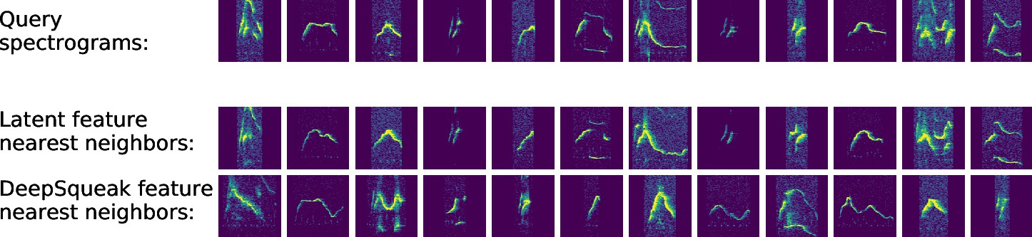
Latent features better represent acoustic similarity.
Top row: example spectrograms; middle row: nearest neighbors in latent space; bottom row: nearest neighbors in DeepSqueak feature space.
Figure 3—figure supplement 1
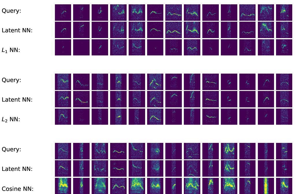
Nearest neighbors returned by distance metrics in spectrogram space exhibit failure modes not found in latent space.
Top block: selected query spectrograms, their nearest neighbors in latent space (Euclidean metric), and their nearest neighbors in spectrogram space (L1 metric). Middle block: same comparison with the L2 metric in spectrogram space. Bottom block: same comparison with the cosine metric in spectrogram space.
Figure 3—figure supplement 2
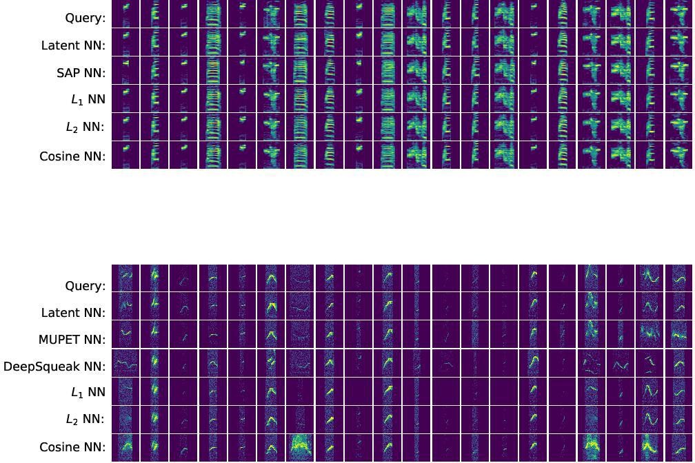
Representative sample of nearest neighbors returned by several feature spaces.
Top block: given 20 random zebra finch syllable spectrograms, we find nearest neighbors in five feature spaces: variational autoencoder (VAE) latent space, Sound Analysis Pro feature space, and spectrogram space (Manhattan [L1], Euclidean [L2], and cosine metrics). All methods consistently find nearest neighbors of the same syllable type. Bottom block: given 20 random mouse syllable spectrograms, we find nearest neighbors in six feature spaces: VAE latent space, MUPET feature space, DeepSqueak feature space, and spectrogram space (Manhattan, Euclidean, and cosine metrics). Most methods return mostly similar spectrograms. However, latent features more consistently return good matches than other methods.
Figure 3—figure supplement 3
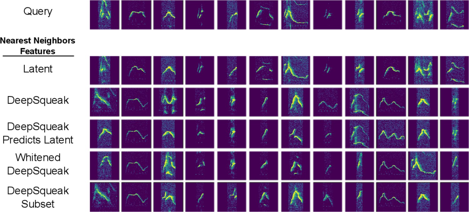
Investigating poor DeepSqueak feature nearest neighbors from Figure 3.
Top row: selected query spectrograms from Figure 3. Lower rows: nearest neighbor spectrograms returned by various feature spaces: latent features, DeepSqueak features Coffey et al., 2019 (standardized, but not whitened), the linear projection of DeepSqueak features that best predicts latent features, whitened DeepSqueak features, and the subset of DeepSqueak features excluding frequency standard deviation, sinuosity, and frequency modulation, the three features most poorly predicted by latent features (Figure 2—figure supplement 1). All three variants of the DeepSqueak feature set return more visually similar nearest neighbors than the original DeepSqueak feature set for some but not all query spectrograms. In particular, the remaining poor nearest neighbors returned by the linear projection of DeepSqueak features most predictive of latent features suggest that DeepSqueak features are insufficient to capture the full acoustic complexity of ultrasonic vocalization syllables.
Figure 4 with 3 supplements
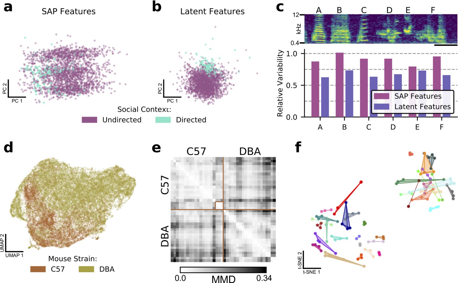
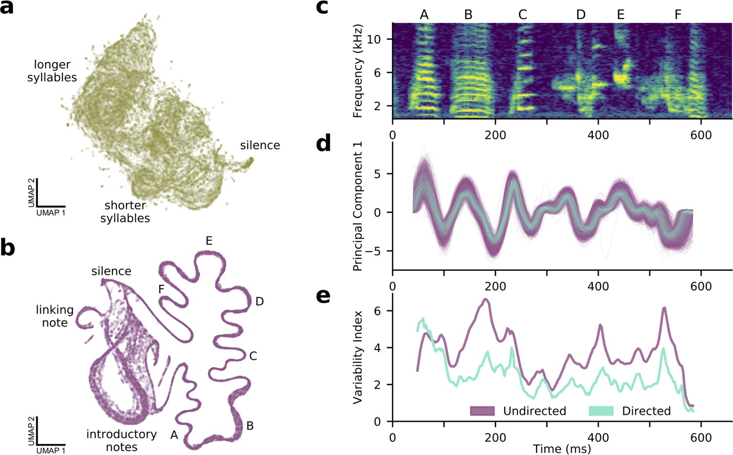
Latent features better capture differences in sets of vocalizations.
(a) The first two principal components in SAP feature space of a single zebra finch song syllable, showing differences in directed and undirected syllable distributions. (b) The first two principal components of latent syllable features, showing the same comparison. Learned latent features more clearly indicate differences between the two conditions by clustering directed syllables together. (c) Acoustic variability of each song syllable as measured by SAP features and latent features (see Methods). Latent features more clearly represent the constriction of variability in the directed context. Spectrogram scale bars denote 100ms. (d) A UMAP projection of the latent means of USV syllables from two strains of mice, showing clear differences in their vocal repertoires. (e) Similarity matrix between syllable repertoires for each of the 40 reccording sessions from (d). Lighter values correspond to more similar syllable repertoires (lower Maximum Mean Discrepancy (MMD)). (f) t-SNE representation of similarities between syllable repertoires, where distance metric is estimated MMD. The dataset, which is distinct from that represented in (d) and (e), contains 36 individuals, 118 recording sessions, and 156,180 total syllables. Color indicates individual mice and scatterpoints of the same color represent repertoires recorded on different days. Distances between points represent the similarity in vocal repertoires, with closer points more similar. We note that the major source of repertoire variability corresponds to genetic background, corresponding to the two distinct clusters (Figure 4—figure supplement 3). A smaller level of variability can be seen across individuals in the same clusters. Individual mice have repertoires with even less variability, indicated by the close proximity of most repertoires for each mouse.
Figure 4—figure supplement 1
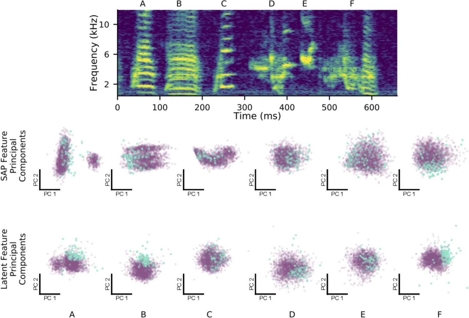
Latent features better represent constricted variability of female-directed zebra finch song.
At top is a single rendition of a male zebra finch’s song motif, with individual syllables labeled (A–F). The top row of scatterplots shows each syllable over many directed (blue) and undirected (purple) renditions, plotted with respect to the first two principal components of the Sound Analysis Pro acoustic feature space. The bottom row of scatterplots shows the same syllables plotted with respect to the first two principal components of latent feature space. The difference in distributions between the two social contexts is displayed more clearly in the latent feature space, especially for non-harmonic syllables (D–F).
Figure 4—figure supplement 2
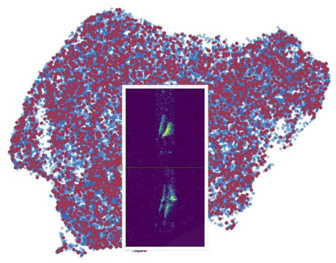
An ‘atlas’ of mouse ultrasonic vocalizations (USVs).
This screenshot shows an interactive version of Figure 4d in which example spectrograms are displayed as tooltips when a cursor hovers over the plot. A version of this plot is hosted at: https://pearsonlab.github.io/research.html#mouse_tooltip.
Figure 4—figure supplement 3
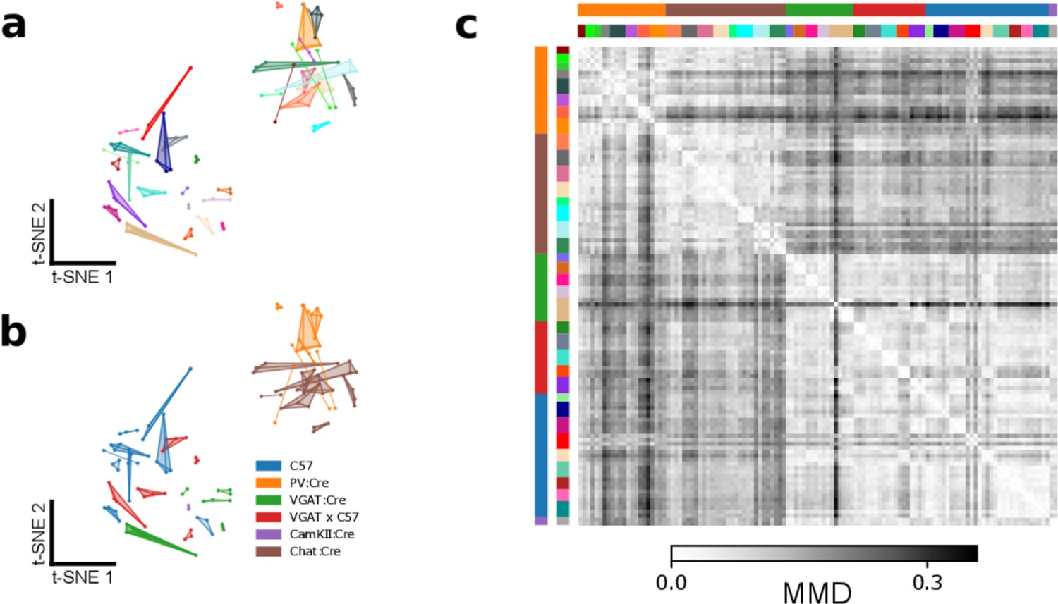
Details of Figure 4f.
(a) t-SNE representation of similarities between syllable repertoires, where distance metric is estimated maximum mean discrepancy (MMD) between latent syllable distributions (reproduction of Figure 4f). Each scatter represents the ultrasonic vocalization (USV) syllable repertoire of a single recording session. Recordings of the same mice across different days are connected and colored identically. Distances between points represent the similarity in vocal repertoires, with closer points more similar. Note that most mice have similar repertoires across days, indicated by the close proximity of connected scatterpoints. (b) The same plot as (a), colored by the genetic background of each mouse. Note that the two primary clusters of USV syllable repertoires correspond to two distinct sets of genetic backgrounds. (c) The full pairwise MMD matrix between USV repertoires from individual recording sessions. The dataset contains 36 individuals, 118 recording sessions, and 156,180 total syllables. The two main clusters separating the PV:Cre and Chat:Cre mice from the other backgrounds are apparent as the large two-by-two checkerboard pattern. Colors at the top and left sides indicate individual and genetic background information, with colors matching those in panels (a) and (b).
Figure 5 with 5 supplements
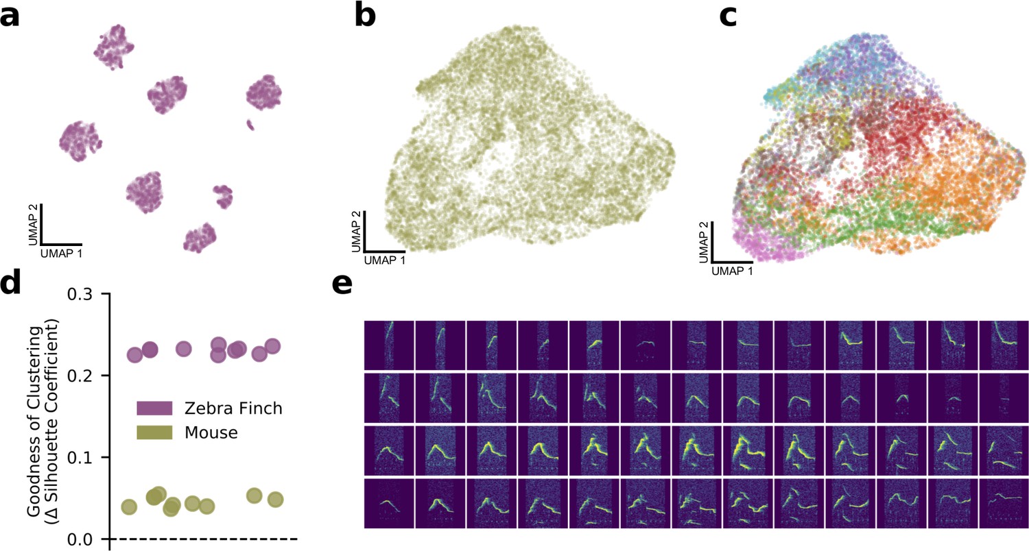
Bird syllables clearly cluster, but mouse ultrasonic vocalizations (USVs) do not.
(a) UMAP projection of the song syllables of a single male zebra finch (14,270 syllables). (b) UMAP projection of the USV syllables of a single male mouse (17,400 syllables). (c) The same UMAP projection as in (b), colored by MUPET-assigned labels. (d) Mean silhouette coefficient (an unsupervised clustering metric) for latent descriptions of zebra finch song syllables and mouse syllables. The dotted line indicates the null hypothesis of a single covariance-matched Gaussian noise cluster fit by the same algorithm. Each scatterpoint indicates a cross-validation fold, and scores are plotted as differences from the null model. Higher scores indicate more clustering. (e) Interpolations (horizontal series) between distinct USV shapes (left and right edges) demonstrating the lack of data gaps between putative USV clusters.
Figure 5—figure supplement 1
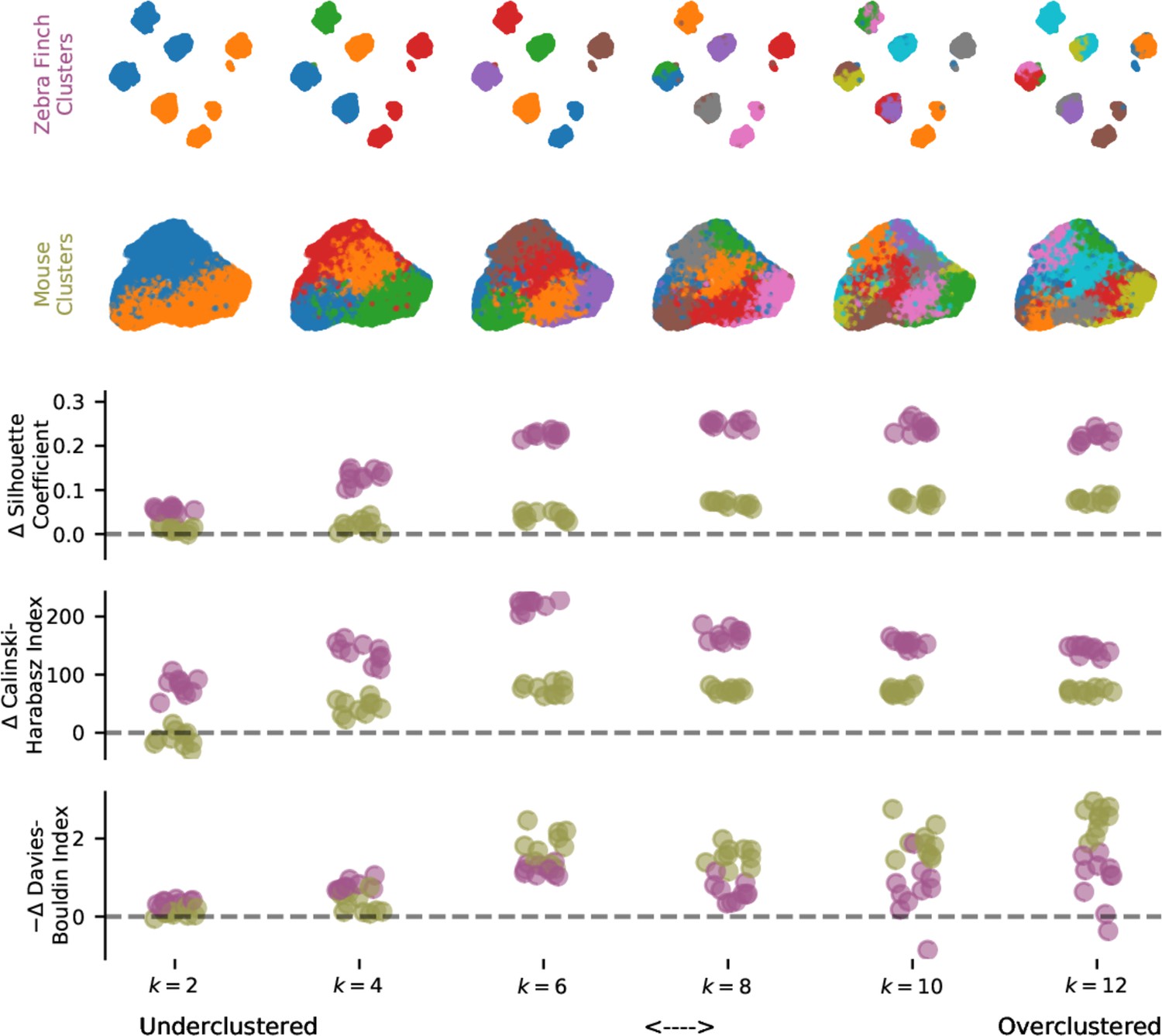
Evaluation of clustering metrics on vocalization for different cluster numbers.
Three unsupervised clustering metrics evaluated on the latent description of zebra finch song syllables (Figure 5a) and mouse ultrasonic vocalization syllables (Figure 5b) as the number of components, , varies from 2 to 12. Clustering metrics are reported relative to moment-matched Gaussian noise (see Materials and methods) with a possible sign change so that higher scores indicate more clustering.
Figure 5—figure supplement 2
Evaluation of clustering metrics on different mouse ultrasonic vocalization (USV) feature sets.
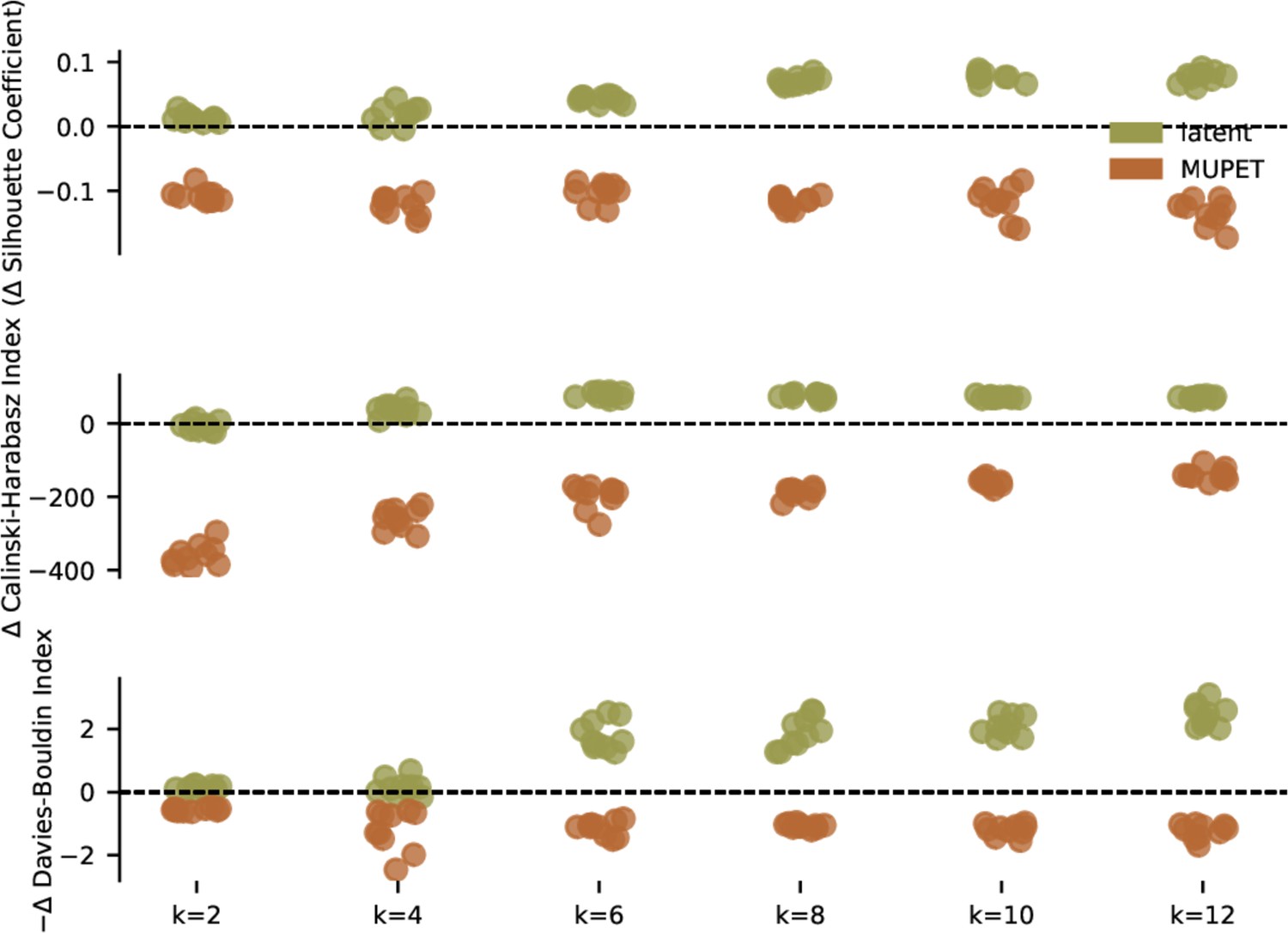
Three unsupervised clustering metrics evaluated on latent and MUPET features of mouse USV syllables (Figure 5b) as the number of components, k, varies from 2 to 12. Clustering metrics are reported relative to moment-matched Gaussian noise (see Materials and methods) with a possible sign change so that higher scores indicate more clustering. Latent features are consistently judged to produce better clustering than MUPET feature. Additionally, MUPET features are consistently judged to be less clustered than moment-matched Gaussian noise. Compare to Figure 5—figure supplement 3.
Figure 5—figure supplement 3
Evaluation of clustering metrics on different zebra finch syllable feature sets.
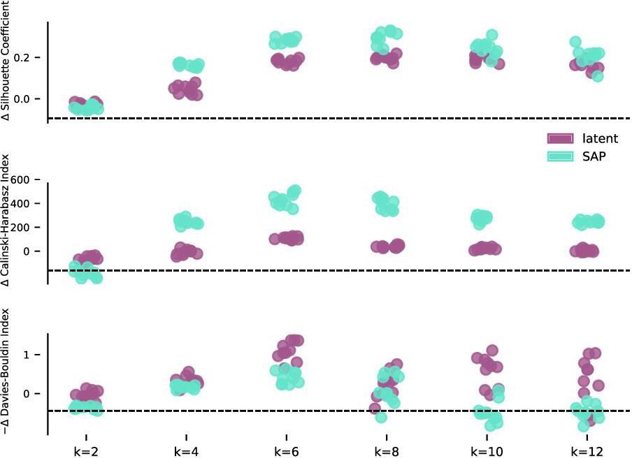
Three unsupervised clustering metrics evaluated on latent and SAP features of zebra finch song syllables (Figure 5a) as the number of components, k, varies from 2 to 12. Clustering metrics are reported relative to moment-matched Gaussian noise (see Materials and methods) with a possible sign change so that higher scores indicate more clustering. Both feature sets admit clusters that are consistently judged to be more clustered than moment-matched Gaussian noise.
Figure 5—figure supplement 4
Reliability of clustering for zebra finch syllables and mouse ultrasonic vocalizations (USVs).
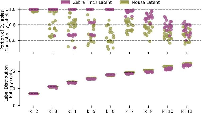
Repeated clustering with Gaussian mixture models (GMMs) produces reliable clusters for zebra finch syllable latent features with six clusters, but not for mouse syllable latent features with more than two clusters. Both sets of syllable latent descriptions (zebra finch, 14,270 syllables; mouse, 15,712 syllables) are repeatedly split into thirds. The first and second splits are used to train GMMs (full covariance, best of five fits, fit via expectation maximization), which are used to predict labels on the third split. Given these predicted labels and a matching of labels between the two GMMs, a syllable can be considered consistently labeled if it is assigned the same label class by the two GMMs. The Hungarian method is used to find the label matching that maximizes the portion of consistently labeled syllables. Top row: the portion of consistently labeled syllables for 20 repetitions of this procedure is shown for varying numbers of clusters, k. Note that zebra finch syllables achieve near-perfect consistency for six clusters, the number of clusters found by hand labeling (syllables A–F in Figure 6c), and this consistency degrades with more clusters. By contrast, the consistency of mouse USV clusters is poor. Somewhat surprisingly, the clustering is very consistent for two clusters (k = 2). To test whether this is a trivial effect of rarely used clusters, we calculated the entropy of the empirical label distributions (bottom row). We find in each case, and specifically the case, that the empirical distribution entropy is close to the maximum possible entropy (plotted as dashed horizontal lines), indicating that all clusters are frequently used. While consistent with mouse USVs forming two clusters, this result is not sufficient proof of syllable clustering or even bimodality. Yet, for cluster identity to be a practical syllable descriptor, clusters should be readily identifiable from the data. Thus the combination of VAE-identified latent features and Gaussian clusters does not appear to be a suitable description of mouse USVs for k > 2 clusters. Note that the portion of consistently labeled zebra finch syllables for k < 6 clusters form well-defined bands at multiples of , indicating that cluster structure is so well defined by the data that the GMMs do not split individual clusters across multiple Gaussian components.
Figure 5—figure supplement 5
Absence of continuous interpolations between zebra finch song syllables.
Each row displays two random zebra finch syllables of different syllable types at either end and an attempted smooth interpolation between the two. Interpolating spectrograms are those with the closest latent features along a linear interpolation in latent space. Note the discontinuous jump in each attempted interpolation, which is expected given that adult zebra finch syllables are believed to be well-clustered. Compare with Figure 5e, which shows continuous variation in mouse ultrasonic vocalizations.
Figure 6 with 4 supplements
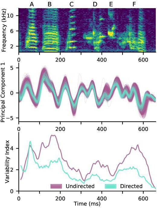
A shotgun variational autoencoder approach learns low dimensional latent representations of subsampled, fixed-duration spectrograms and captures short-timescale variability in behavior.
(a) A UMAP projection of 100,000 200-ms windows of mouse ultrasonic vocalizations (cp. Figure 4a). (b) A UMAP projection of 100,000 120-ms windows of zebra finch song (cp. Figure 4b). Song progresses counterclockwise on the right side, while more variable, repeated introductory notes form a loop on the left side. (c) A single rendition of the song in (b). (d) The song’s first principal component in latent space, showing both directed (cyan) and undirected (purple) renditions. (e) In contrast to a syllable-level analysis, the shotgun approach can measure zebra finch song variability in continuous time. Song variability in both directed (cyan) and undirected (purple) contexts is plotted (see Materials and methods).
Figure 6—figure supplement 1
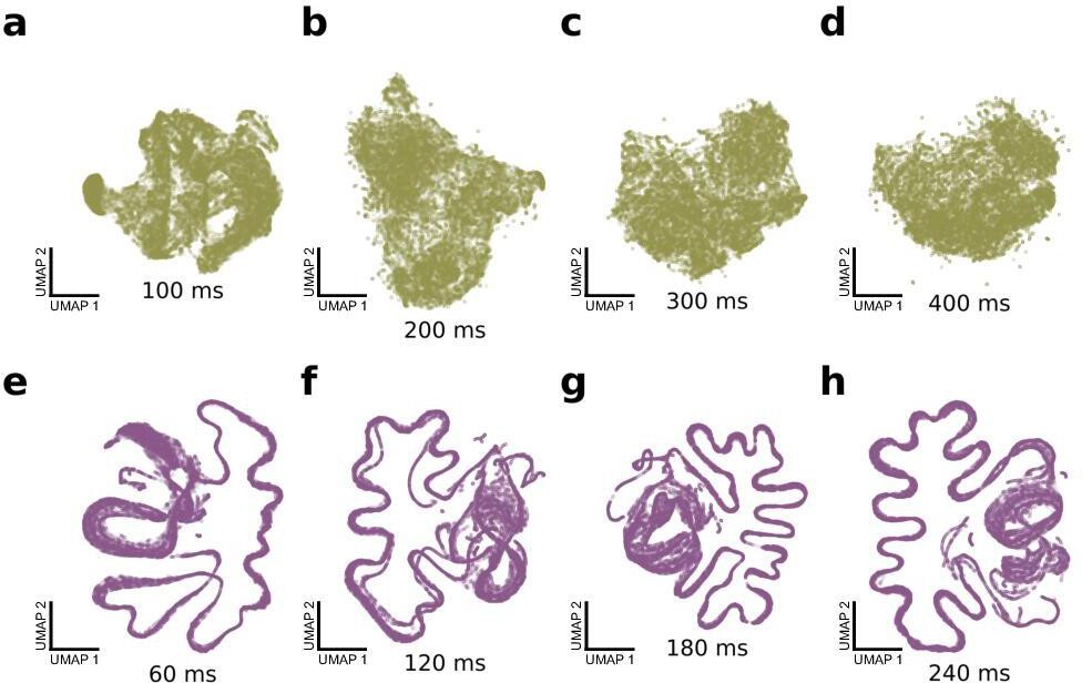
Effect of window duration on shotgun variational autoencoder (VAE).
Qualitatively similar shotgun VAE latent projections are achieved with a wide range of window durations. (a–d) UMAP projections of 100,000 windows of mouse ultrasonic vocalizations, with window durations of 100, 200, 300, and 400 ms. Compare with Figure 6a. (e–h) UMAP projections of 100,000 windows of zebra finch song motifs, with window durations of 60, 120, 180, and 240 ms. Compare with Figure 6b.
Figure 6—figure supplement 2
Effect of time warping on shotgun variational autoencoder.
Non-timewarped version of Figure 6c-e. As in Figure 6d, there is reduced variability in the first latent principal component for directed song compared to undirected song. The overall variability reduction is quantified by the variability index (see Materials and methods), reproducing the reduced variability of directed song found in Figure 6e. Note that the directed traces lag the undirected traces at the beginning of the motif and lead at the end of the motif due to their faster tempo, which is uncorrected in this version of the analysis.
Figure 6—video 1
An animated version of Figure 6b.
Recorded USVs from asingle male mouse are played while the corresponding latent features are visualized by a moving star in a UMAP projection of latent space. The recording is slowed by a factor of four and additionally pitchshifted downward by a factor of two so that the vocalizations areaudible.
Figure 6—video 2
An animated version of Figure 6a.
A recorded song boutfrom a single male zebra finch is played while the corresponding latent features are visualized by a moving star in a UMAP projectionof latent space.
Figure 7 with 3 supplements
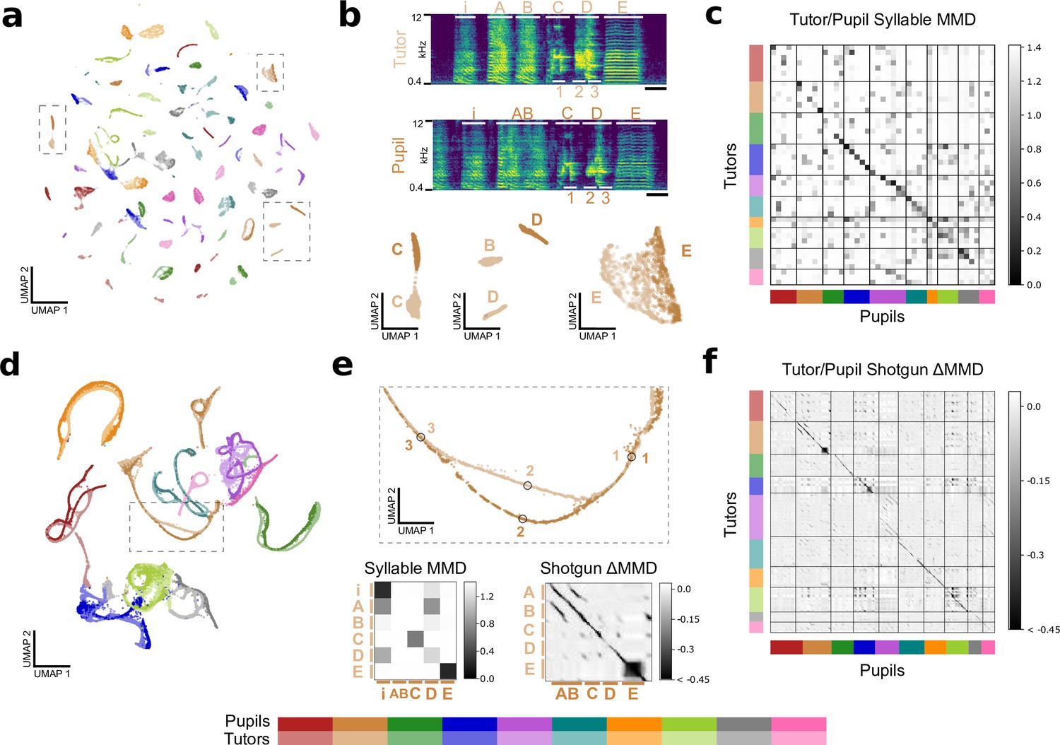
Latent features capture similarities between tutor and pupil song.
(a) Latent UMAP projection of the song syllables of 10 zebra finch tutor/pupil pairs. Note that many tutor and pupil syllables cluster together, indicating song copying. (b) Example song motifs from one tutor/pupil pair. Letters A-E indicate syllables. Syllables Syllables “C” and “E” are well-copied, but the pupil’s rendition of syllable “D” does not have as much high-frequency power as the tutor’s rendition. The difference between these two renditions is captured in the latent UMAP projection below. Additionally, the pupil sings a concatenated version of the tutor’s syllables “A” and “B,” a regularity that a syllable-level analysis cannot capture. Thus, the pupil’s syllable “AB” does not appear near tutor syllable “B” in the UMAP projection. Scale bar denotes 100ms. (c) Quality of song copying, estimated by maximum mean discrepancy (MMD) between every pair of tutor and pupil syllables. The dark band of low MMD values near the diagonal indicates good song copying. Syllables are shown in motif order. (d) Latent UMAP projection of shotgun VAE latents (60ms windows) for the song motifs of 10 zebra finch tutor/pupil pairs. Song copying is captured by the extent to which pupil and tutor strands co-localize. (e) Top: Detail of the UMAP projection in panel d shows a temporary split in pupil and tutor song strands spanning the beginning of syllable “D” with poorly copied high-frequency power. Labeled points correspond to the motif fragments marked in panel b. Bottom: Details of the syllable and shotgun MMD matrices in panels c and f. Note high MMD values for the poorly copied “D” syllable. Additionally, the syllable-level analysis reports high MMD betwen the pupil’s fused “AB” and syllable and tutor’s“A” and “B” syllables, though the shotgun VAE approach reports high similarity (low MMD) between pupil andtutor throughout these syllables. (f) MMD between pupil and tutor shotgun VAE latents indexed by continuous-valued time-in-motif quantifies song copying on fine timescales. The dark bands near the diagonal indicate well-copied stretches of song. The deviation of MMD values from a rank-one matrix is displayed for visual clarity (see Figure 7—figure supplement 2 for details). Best viewed zoomed in.
Figure 7—figure supplement 1
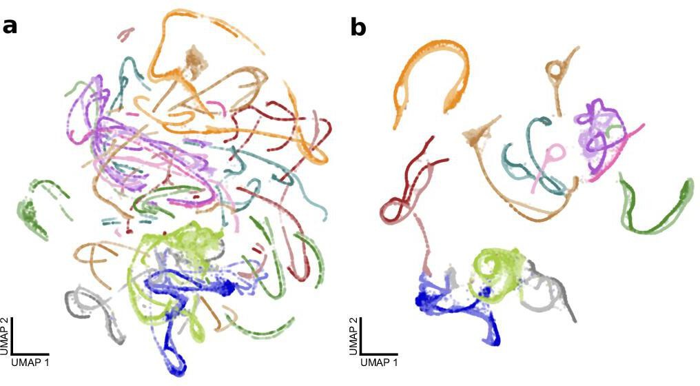
Effect of modified UMAP distance matrix on shotgun variational autoencoder (VAE) from Figure 7d,e.
(a) A UMAP projection of shotgun VAE latent means with a standard Euclidean metric. Colors represent birds as in Figure 7. (b) A UMAP projection of the same latent means with a modified metric to discourage strands from the same motif rendition from splitting (see Materials and methods). This is a reproduction of Figure 7d.
Figure 7—figure supplement 2
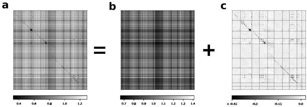
Full and rank-one estimates of maximum mean discrepancy (MMD) matrix.
For the shotgun variational autoencoder pupil/tutor analysis presented in Figure 7, an MMD matrix (a) is decomposed into a rank-one component (b) and a residual component (c). The residual component is shown in Figure 7f for visual clarity. The decomposition is performed by MAP estimation assuming a flat prior on the rank-one matrix and independent Laplace errors on the residual component.
Figure 7—video 1
An animated version of Figure 7d.
Tables
Appendix 1—table 1
Comparison of feature sets on the downstream task of predicting finch social context.
(directed vs. undirected context) given acoustic features of single syllables.Classification accuracy, in percent, averaged over five disjoint, class-balanced splits of the data is reported. Empirical standard deviation is shown in parentheses. Euclidean distance is used for nearest neighbor classifiers. Each SAP acoustic feature is independently z-scored as a preprocessing step. Latent feature dimension is truncated when >99% of the feature variance is explained. Random forest (RF) classifiers use 100 trees and the Gini impurity criterion. The multilayer perceptron (MLP) classifiers are two-layer networks with a hidden layer size of 100, ReLU activations, and an L2 weight regularization parameter ‘alpha,’ trained with ADAM optimization with a learning rate of 10-3 for 200 epochs. D denotes the dimension of each feature set, with Gaussian random projections used to decrease the dimension of spectrograms.
| Predicting finch social context (Figure 4a–c) | |||||
|---|---|---|---|---|---|
| Spectrogram | SAP | Latent | |||
| D = 10 | D = 30 | D = 100 | D = 13 | D = 5 | |
| k-NN () | 92.5 (0.2) | 95.3 (0.1) | 97.3 (0.3) | 93.0 (0.3) | 96.9 (0.2) |
| -NN () | 93.0 (0.2) | 95.3 (0.2) | 97.1 (0.3) | 93.2 (0.1) | 96.7 (0.2) |
| -NN () | 92.7 (0.1) | 94.2 (0.2) | 96.0 (0.2) | 92.8 (0.1) | 96.3 (0.1) |
| RF (depth = 10) | 92.6 (0.1) | 92.7 (0.1) | 93.1 (0.1) | 92.8 (0.1) | 94.9 (0.2) |
| RF (depth = 15) | 92.7 (0.1) | 93.2 (0.2) | 93.6 (0.1) | 93.6 (0.2) | 96.1 (0.1) |
| RF (depth = 20) | 92.8 (0.1) | 93.4 (0.1) | 93.8 (0.1) | 93.8 (0.2) | 96.4 (0.2) |
| MLP (α = 0.1) | 92.8 (0.4) | 95.4 (0.4) | 97.6 (0.3) | 92.9 (0.1) | 95.7 (0.1) |
| MLP (α = 0.01) | 92.9 (0.3) | 95.4 (0.3) | 97.5 (0.2) | 93.1 (0.2) | 96.2 (0.1) |
| MLP (α = 0.001) | 92.7 (0.6) | 95.2 (0.5) | 97.5 (0.2) | 93.0 (0.2) | 96.3 (0.0) |
Appendix 1—table 2
Comparison of feature sets on the downstream task of predicting mouse strain.
(C57 vs.DBA) given acoustic features of single syllables. Classification accuracy, in percent, averaged over five disjoint, class-balanced splits of the data is reported. Empirical standard deviation is shown in parentheses. Euclidean distance is used for nearest neighbor classifiers. Each MUPET and DeepSqueak acoustic feature is independently z-scored as a preprocessing step. Latent features dimension is truncated when >99% of the feature variance is explained. Random forest (RF) classifiers use 100 trees and the Gini impurity criterion. The multilayer perceptron (MLP) classifiers are two-layer networks with a hidden layer size of 100, ReLU activations, and an L2 weight regularization parameter ‘alpha,’ trained with ADAM optimization with a learning rate of 10-3 for 200 epochs. D denotes the dimension of each feature set, with Gaussian random projections used to decrease the dimension of spectrograms.
| Predicting mouse strain (Figure 4d–e) | ||||||
|---|---|---|---|---|---|---|
| Spectrogram | MUPET | DeepSqueak | Latent | |||
| D = 10 | D = 30 | D = 100 | D = 9 | D = 10 | D = 7 | |
| -NN () | 68.1 (0.2) | 76.4 (0.3) | 82.3 (0.5) | 86.1 (0.2) | 79.0 (0.3) | 89.8 (0.2) |
| -NN () | 71.0 (0.3) | 78.2 (0.1) | 82.7 (0.6) | 87.0 (0.1) | 80.7 (0.3) | 90.7 (0.4) |
| -NN () | 72.8 (0.3) | 78.5 (0.2) | 81.3 (0.5) | 86.8 (0.2) | 81.0 (0.2) | 90.3 (0.4) |
| RF (depth = 10) | 72.8 (0.2) | 76.6 (0.2) | 79.1 (0.3) | 87.4 (0.5) | 81.2 (0.4) | 88.1 (0.5) |
| RF (depth = 15) | 73.1 (0.3) | 78.0 (0.3) | 80.5 (0.2) | 87.9 (0.4) | 82.1 (0.3) | 89.6 (0.4) |
| RF (depth = 20) | 73.2 (0.2) | 78.3 (0.2) | 80.7 (0.3) | 87.9 (0.4) | 81.9 (0.3) | 89.6 (0.4) |
| MLP (α = 0.1) | 72.4 (0.3) | 79.1 (0.4) | 84.5 (0.3) | 87.8 (0.2) | 82.1 (0.4) | 90.1 (0.3) |
| MLP (α = 0.01) | 72.3 (0.4) | 78.6 (0.3) | 82.9 (0.4) | 88.1 (0.3) | 82.4 (0.4) | 90.0 (0.4) |
| MLP (α = 0.001) | 72.4 (0.4) | 78.5 (0.8) | 82.8 (0.1) | 87.9 (0.2) | 82.4 (0.3) | 90.4 (0.3) |
Appendix 1—table 3
Comparison of feature sets on the downstream task of predicting mouse identity given acoustic features of single syllables.
Classification accuracy, in percent, averaged over five disjoint, class-balanced splits of the data is reported. A class-weighted log-likelihood loss is targeted to help correct for class imbalance. Empirical standard deviation is shown in parentheses. Each MUPET acoustic feature is independently z-scored as a preprocessing step. Latent feature principal components are truncated when >99% of the feature variance is explained. The multilayer perceptron (MLP) classifiers are two-layer networks with a hidden layer size of 100, ReLU activations, and an L2 weight regularization parameter ‘alpha,’ trained with ADAM optimization with a learning rate of 10-3 for 200 epochs. Chance performance is 2.8% for top-1 accuracy and 13.9% for top-5 accuracy. D denotes the dimension of each feature set, with Gaussian random projections used to decrease the dimension of spectrograms.
| Predicting mouse identity (Figure 4f) | |||||
|---|---|---|---|---|---|
| Spectrogram | MUPET | Latent | |||
| D = 10 | D = 30 | D = 100 | D = 9 | D = 8 | |
| Top-1 accuracy | |||||
| MLP (α = 0.01) | 9.9 (0.2) | 14.9 (0.2) | 20.4 (0.4) | 14.7 (0.2) | 17.0 (0.3) |
| MLP (α = 0.001) | 10.8 (0.1) | 17.3 (0.4) | 25.3 (0.3) | 19.0 (0.3) | 22.7 (0.5) |
| MLP (α = 0.0001) | 10.7 (0.2) | 17.3 (0.3) | 25.1 (0.3) | 20.6 (0.4) | 24.0 (0.2) |
| Top-5 accuracy | |||||
| MLP (α = 0.01) | 36.6 (0.4) | 45.1 (0.5) | 55.0 (0.3) | 46.5 (0.3) | 49.9 (0.4) |
| MLP (α = 0.001) | 38.6 (0.2) | 50.7 (0.6) | 62.9 (0.4) | 54.0 (0.2) | 59.2 (0.6) |
| MLP (α = 0.0001) | 38.7 (0.5) | 50.8 (0.3) | 63.2 (0.4) | 57.3 (0.4) | 61.6 (0.4) |
Additional files
Download links
A two-part list of links to download the article, or parts of the article, in various formats.
Downloads (link to download the article as PDF)
Open citations (links to open the citations from this article in various online reference manager services)
Cite this article (links to download the citations from this article in formats compatible with various reference manager tools)
Low-dimensional learned feature spaces quantify individual and group differences in vocal repertoires
eLife 10:e67855.
https://doi.org/10.7554/eLife.67855


