Figures and data in Direct extraction of signal and noise correlations from two-photon calcium imaging of ensemble neuronal activity

Figures
Tables
Additional files

8 figures, 3 tables and 1 additional file

Figures

Figure 1

Download asset Open asset

The proposed generative model and inverse problem.

Observed (green) and latent (orange) variables pertinent to the $j^{𝗍𝗁}$ neuron are indicated, according to the proposed model for estimating the signal (blue) and noise (red) correlations from two-photon calcium fluorescence observations. Calcium fluorescence traces $(y_{t, l}^{(j)})$ of $L$ trials are observed, in which the repeated external stimulus $(𝐬_{t})$ is known. The underlying spiking activity $(n_{t, l}^{(j)})$ , trial-to-trial variability and other intrinsic/extrinsic neural covariates that are not time-locked with the external stimulus $(x_{t, l}^{(j)})$ , and the stimulus kernel $(𝐝_{j})$ are latent. Our main contribution is to solve the inverse problem: recovering the underlying latent signal $(𝐒)$ and noise $(𝐍)$ correlations directly from the fluorescence observations, without requiring intermediate spike deconvolution.

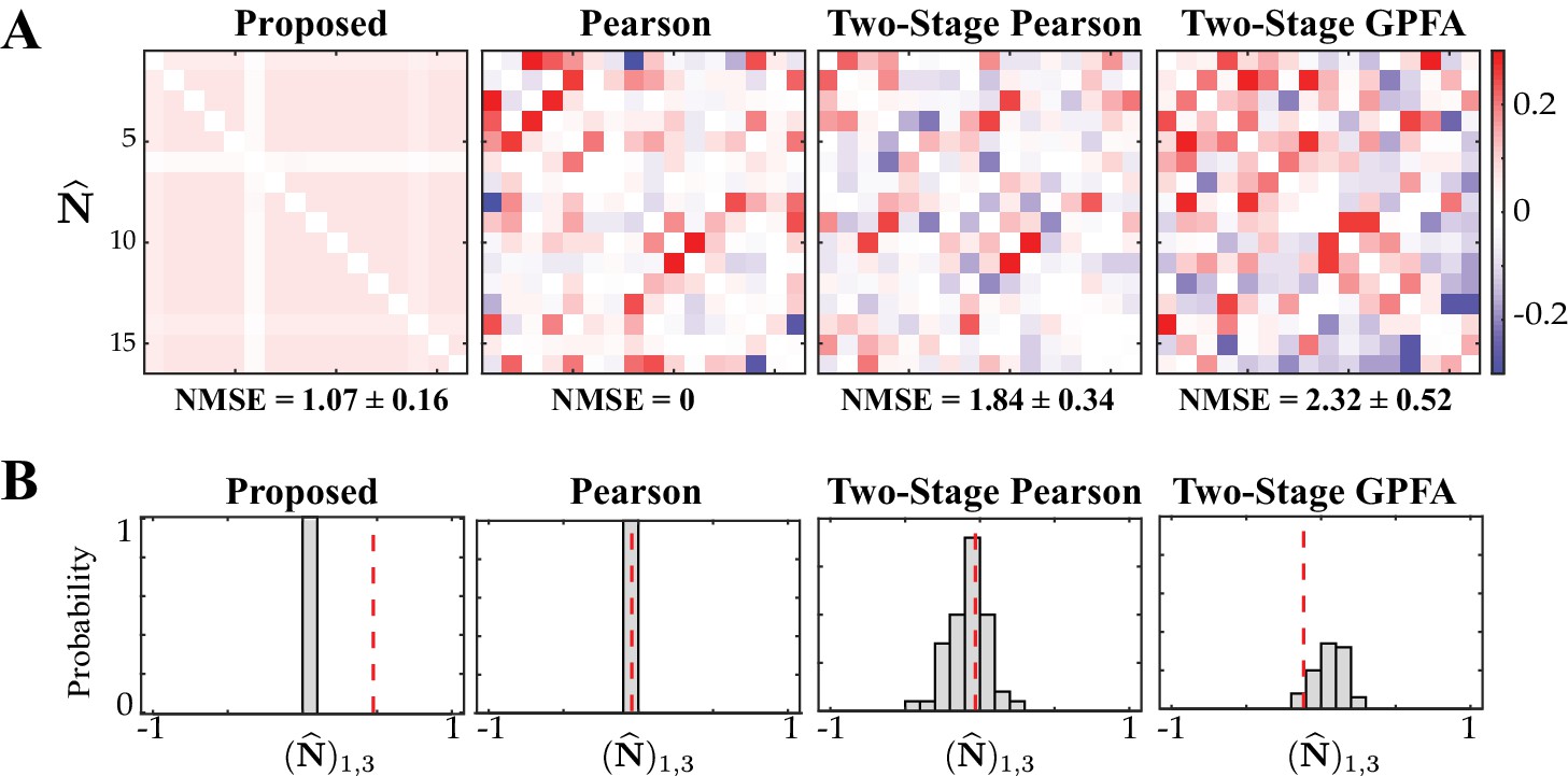
Figure 2 with 6 supplements

Download asset Open asset

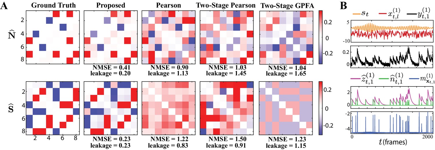
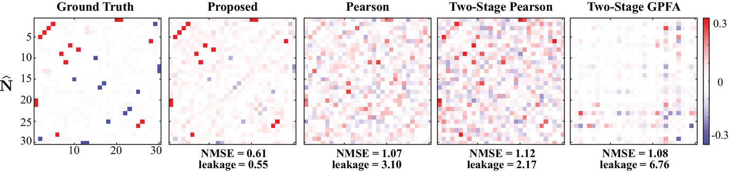
Results of simulation study 1.

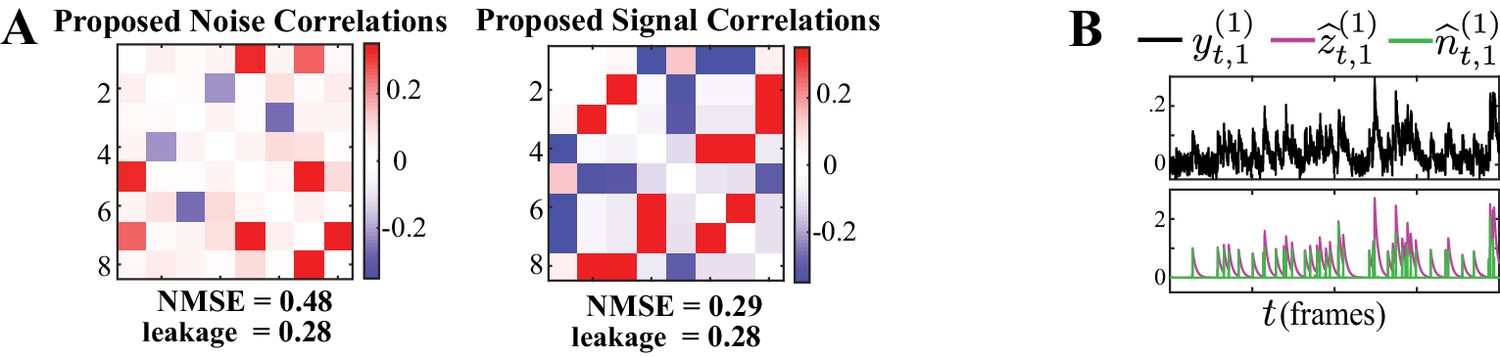
(A) Estimated noise and signal correlation matrices from different methods. Rows from left to right: ground truth, proposed method, Pearson correlations from two-photon recordings, two-stage Pearson estimates and two-stage GPFA estimates. The normalized mean squared error (NMSE) of each estimate with respect to the ground truth and the leakage effect quantified by the ratio between out-of-network and in-network power (leakage) are indicated below each panel. (B) Simulated external stimulus (orange), latent trial-dependent process (red), fluorescence observations (black), estimated calcium concentrations (purple), putative spikes (green), and estimated mean of the latent state (blue) by the proposed method, for the first trial of neuron 1.

Figure 2—figure supplement 1

Download asset Open asset

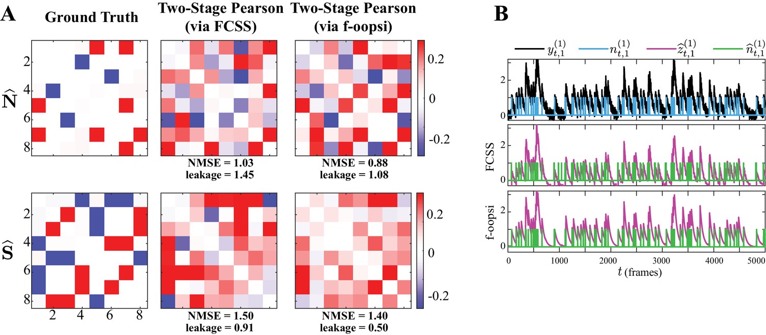
Sensitivity of two-stage estimates to the choice of the underlying spike deconvolution technique.

(A) Noise (first row) and signal (second row) correlations corresponding to the ground truth (first column), estimated by the two-stage Pearson method using the FCSS (Kazemipour et al., 2018) (second column) and constrained f-oopsi (Pnevmatikakis et al., 2016) (third column) spike deconvolution techniques, for the simulation study in Figure 2. The NMSE and leakage ratios of the estimates are indicated below each panel. While the correlation estimates based on these two methods are comparable, there exist notable differences between them, as a result of the slight discrepancies in the deconvolved spikes. This demonstrates that the two-stage estimates are sensitive to minor differences in the estimated spikes obtained by different deconvolution techniques. In addition, both two-stage Pearson estimates fail to capture the ground truth correlations (as is also evident from the high NMSE and leakage values). (B) Simulated observations (black, re-scaled for ease of visual comparison) and ground truth spikes (blue), as well as the estimated calcium concentrations (purple) and putative spikes (green) for the 1st trial of neuron one in the simulation study of Figure 2, using the FCSS (Kazemipour et al., 2018) (second row) and constrained f-oopsi (Pnevmatikakis et al., 2016) (third row) spike deconvolution methods.

Figure 2—figure supplement 2

Download asset Open asset

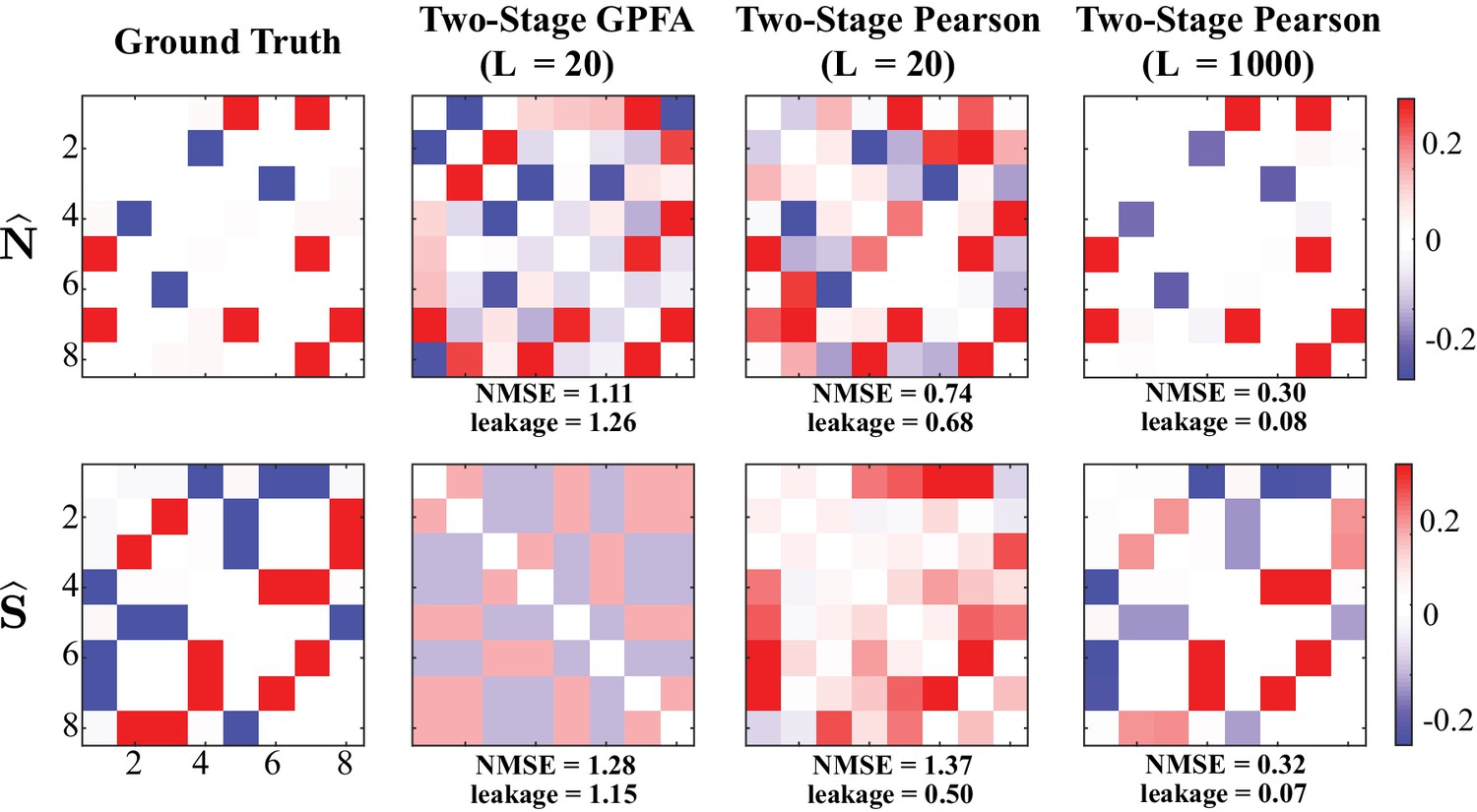
Performance of two-stage estimates based on ground truth spikes.

Performance of two stage estimates based on ground truth spikes. Noise (first row) and signal (second row) correlations corresponding to the ground truth (first column) are repeated from Figure 2. The second and third columns show the results of two-stage GPFA and two-stage Pearson methods using $L = 20$ trials, respectively. The fourth column shows the results of the two-stage Pearson method using $L = 1000$ trials. All estimates were obtained using the ground truth spikes, as opposed to extracting the spikes via a deconvolution technique. Thus, these results isolate the effect of the non-linearities involved in spike generation on the estimation performance. The NMSE and leakage ratios of the estimates are indicated below each panel. Even though the ground truth spikes are used, the NMSE and leakage ratios indicated in the second and third columns are remarkably high. This further shows that the usage of conventional definitions and GPFA estimates is not optimal for the recovery of signal and noise correlations. In accordance with our theoretical analysis in Direct Extraction of Signal and Noise Correlations from Two-Photon Calcium Imaging of Ensemble Neuronal Activity, the performance of the two-stage Pearson method significantly improves as the number of trials is increased to $L = 1000$ , a number that is unrealistic in the context of typical two-photon imaging experiments. However, our proposed method shown in Figure 2 achieves comparable performance with number of trials as low as $L = 20$ . In summary, these results suggest that the two-stage methods produce highly biased estimates under limited number of trials, even if the ground truth spikes were ideally deconvolved from the two-photon data.

Figure 2—figure supplement 3

Download asset Open asset

Performance comparison under stimulus integration model mismatch.

Estimated noise and signal correlation matrices from different methods based on data generated with non-linear stimulus integration. Spikes were generated by replacing the linear receptive field model $𝐝_{j}^{⊤} 𝐬_{t}$ with a non-linear one given by $𝐝_{j}^{⊤} 𝐬_{t} + {({\tilde{𝐝}}_{j, 1}^{⊤} 𝐬_{t})}^{2} + {({\tilde{𝐝}}_{j, 2}^{⊤} 𝐬_{t})}^{2}$ , but a linear stimulus model was used for estimation (i.e., ${\tilde{𝐝}}_{j, 1} = {\tilde{𝐝}}_{j, 2} =$ ). Rows from left to right: ground truth, proposed method, Pearson correlations from two-photon recordings, two-stage Pearson estimates and two-stage GPFA estimates. The normalized mean squared error (NMSE) of each estimate with respect to the ground truth and the leakage effect quantified by the ratio between out-of-network and in-network power (leakage) are indicated below each panel. While the NMSE in our proposed signal correlation estimates under this setting is greater than that in Figure 2 with no model mismatch, our proposed estimates still outperform existing methods. In addition, model mismatch in the stimulus integration component does not affect the accuracy of noise correlations estimated by our method.

Figure 2—figure supplement 4

Download asset Open asset

Performance under calcium decay model mismatch.

(A) Proposed noise and signal correlation estimates for data simulated at lower SNR than the setting of Figure 2 and model mismatch introduced by using a second-order autoregressive model for the calcium decay. The ground truth correlations are the same as those in Figure 2. The NMSE and leakage ratio are given at the bottom. (B) Putative spikes (green) and estimated calcium concentrations (purple). The model mismatch and lower SNR result in slight performance degradation compared to Figure 2 (in terms of NMSE and leakage), and our method is capable of recovering the underlying correlations faithfully.

Figure 2—figure supplement 5

Download asset Open asset

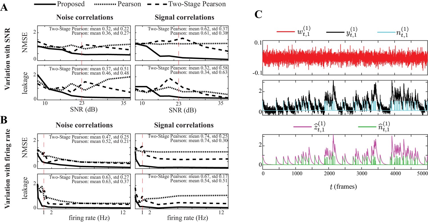
Performance comparison under varying SNR levels and firing rates.

Performance comparison with respect to varying SNR levels and average firing rates. (A) NMSE (top) and leakage ratios (bottom) for the noise (left) and signal (right) correlation estimates vs. SNR (in dB), for the proposed method, Pearson correlations from two-photon data and two-stage Pearson method. The SNR setting corresponding to Figure 2 is indicated by a dashed vertical line. The mean and standard deviation (std) of the normalized performance gain of the proposed method in comparison to the two existing methods are indicates as insets in each panel. (B) Same organization as panel A, but with respect to varying firing rates (in Hz). (C) Sample simulated white observation noise (red), two-photon observations (black, re-scaled for ease of visual comparison) and ground truth spikes (blue), as well as the estimated calcium concentrations (purple) and putative spikes (green) for the 1st trial of neuron 1. While the performance of all methods degrade at low SNR levels or firing rates (SNR lt₁₀ dB, firing rate lt_0.5 Hz), our proposed method outperforms the existing methods for almost all SNR and firing rate settings considered.

Figure 2—figure supplement 6

Download asset Open asset

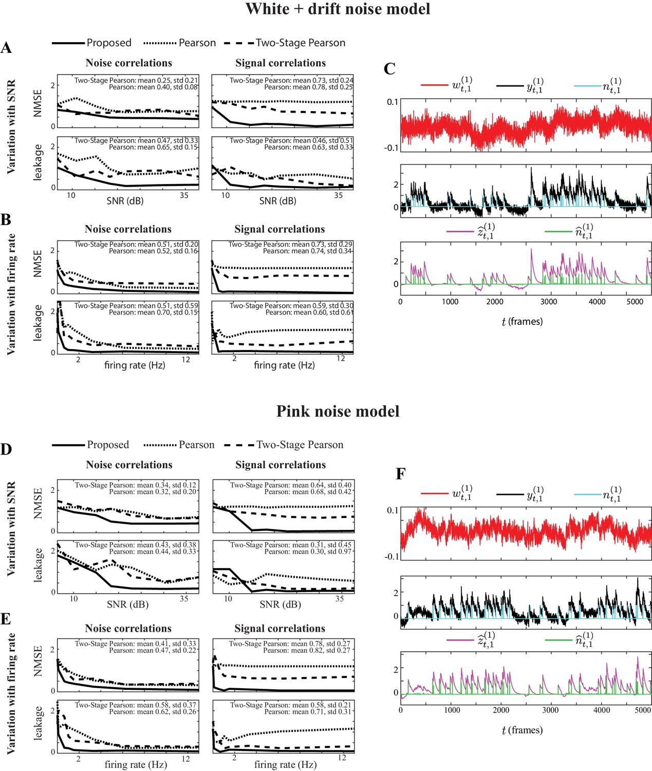
Performance comparison under observation noise model mismatch.

Performance comparison with respect to varying SNR levels and average firing rates, with additional observation noise model mismatch. (A) NMSE (top) and leakage ratios (bottom) for the noise (left) and signal (right) correlation estimates vs. SNR (in dB), for the proposed method, Pearson correlations from two-photon data and two-stage Pearson method. The observation noise is generated by a white noise signal with an additive drift component from a low-frequency auto-regressive process. The mean and standard deviation (std) of the normalized performance gain of the proposed method in comparison to the two existing methods are indicates as insets in each panel. (B) Same organization as panel A, but with respect to varying firing rates (in Hz). (C) Sample simulated observation noise (red), two-photon observations (black, re-scaled for ease of visual comparison) and ground truth spikes (blue), as well as the estimated calcium concentrations (purple) and putative spikes (green) for the 1st trial of neuron 1. Panels (D), (E), and (F) are respectively in the same organization as panels (A), (B), and (C), but the observation noise is generated by a pink noise process. Our proposed method outperforms the existing methods for a wide range of SNR and firing rate values and under both observation noise model mismatch conditions.

Figure 3

Download asset Open asset

Results of simulation study 2.

Estimated noise correlation matrices using different methods based from spontaneous activity data. Rows from left to right: ground truth, proposed method, Pearson correlations from two-photon recordings, two-stage Pearson and two-stage GPFA estimates. The normalized mean squared error (NMSE) of each estimate with respect to the ground truth and the ratio between out-of-network power and in-network power (leakage) are shown below each panel.

Figure 4 with 2 supplements

Download asset Open asset

Application to experimentally-recorded data from the mouse A1.

(A) Estimated noise (top) and signal (bottom) correlation matrices using different methods. Rows from left to right: proposed method, Pearson correlations from two-photon data, two-stage Pearson and two-stage GPFA estimates. (B) Location of the selected neurons with the highest activity in the field of view. (C) Presented tone sequence (orange), observations (black), estimated calcium concentrations (purple), putative spikes (green) and estimated mean latent state (blue) in the first trial of the first neuron. (D) Null distributions of chance occurrence of dissimilarities between signal and noise correlation estimates using different methods. The observed test statistic in each case is indicated by a dashed vertical line. (E) Scatter plots of signal vs. noise correlations for individual cell pairs (blue dots) corresponding to each method. Data were normalized for comparison by computing z-scores. For each case, the linear regression model fit is shown in red, and the slope and p-value of the t-test are indicated as insets.

Figure 4—figure supplement 1

Download asset Open asset

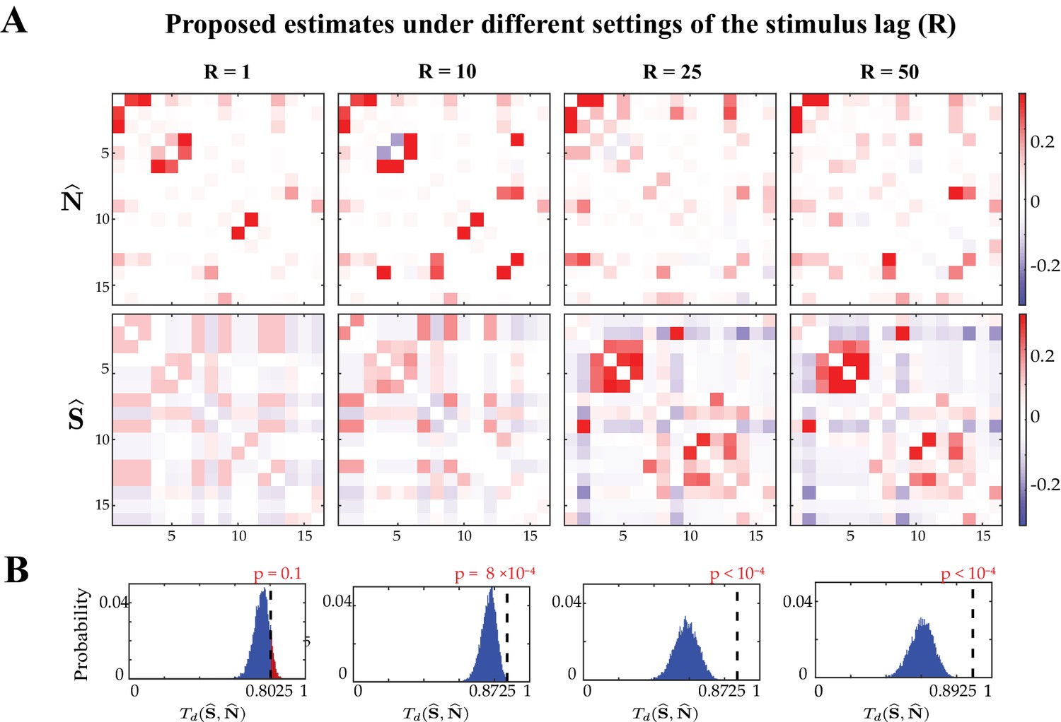
Probing the effect of stimulus integration window length on the performance of the proposed estimates.

Proposed noise and signal correlation estimates under different settings of the stimulus integration window length ( $R$ ). (A) Proposed noise correlation (top) and signal correlation (bottom) estimates under different settings of $R$ , from left to right: $R = 1$ , $R = 10$ , $R = 25$ and $R = 50$ . (B) Null distributions of dissimilarities between proposed signal and noise correlation estimates corresponding to different choice of $R$ . The observed test statistic in each case is indicated by a dashed vertical line, and the p-values are indicated above each panel. These results show that small values of $R = 1$ and $R = 10$ are not adequate to capture stimulus effect. However, both signal and noise correlation estimates exhibit consistency for $R = 25$ and $R = 50$ .

Figure 4—figure supplement 2

Download asset Open asset

Inspecting the inferred latent processes under high fluorescence activity due to rapid increase in firing rate.

The fluorescence observations (black), inferred calcium concentrations (purple) and putative spikes (green) by our proposed method, for a sample data segment with high fluorescence activity due to successive closely spaced spikes. The rise onset of the fluorescence activity is marked by the vertical dashed line and spiking magnitude level of 1 is indicated by the horizontal dashed line. The proposed method favorably recovers the underlying calcium concentrations by predicting putative spikes in successive windows following the rapid rise of the fluorescence and with magnitudes possibly larger than 1.

Figure 5

Download asset Open asset

Assessing the specificity of different estimation results shown in Figure 4.

Rows from left to right: proposed method, Pearson correlations from two-photon data, two-stage Pearson and two-stage GPFA estimates. (A) The estimated noise correlations using different methods after random temporal shuffling of the observations. The mean and standard deviation of the NMSE across 50 trials are indicated below each panel. (B) Histograms of the noise correlation estimates between the first and third neurons over the 50 temporal shuffling trials. The estimate based on the original (un-shuffled) data in each case is indicated by a dashed vertical line.

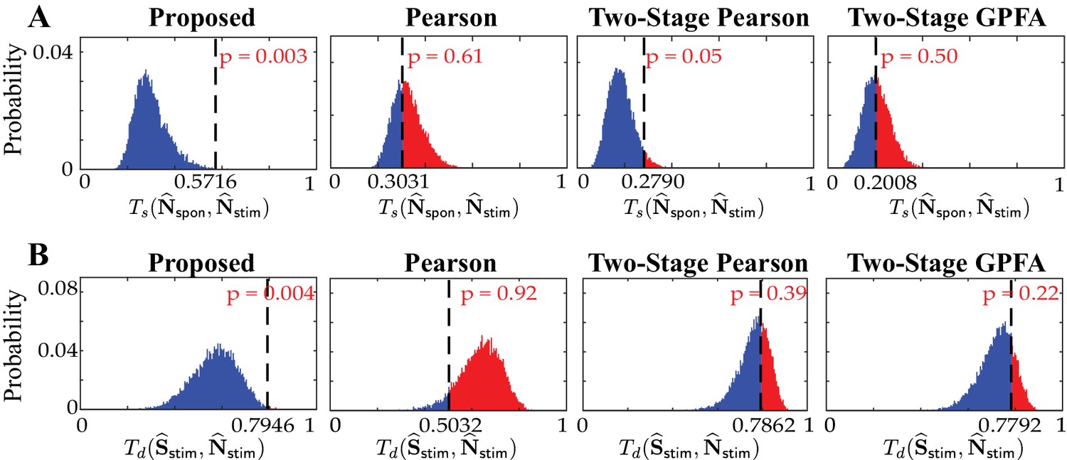
Figure 6 with 1 supplement

Download asset Open asset

Comparison of spontaneous and stimulus-driven activity in the mouse A1.

(A) A sample trial sequence in the experiment. Stimulus-driven (stim) trials were recorded with randomly interleaved spontaneous (spon) trials of the same duration. (B) Estimated noise and signal correlation matrices under spontaneous (top) and stimulus-driven (bottom) conditions. Rows from left to right: proposed method, Pearson correlations from two-photon data, two-stage Pearson and two-stage GPFA estimates. (C) Location of the selected neurons with highest activity in the field of view. (D) Stimulus onsets (orange), observations (black), estimated calcium concentrations (purple) and putative spikes (green) for the first trial from two pairs of neurons with high signal correlation (top) and high noise correlation (bottom), as identified by the proposed estimates.

Figure 6—figure supplement 1

Download asset Open asset

Histograms of the similarity/dissimilarity metrics under the shuffling procedure.

Null distributions of (A) the similarities between $𝐍_{𝗌𝗉𝗈𝗇}$ and $𝐍_{𝗌𝗍𝗂𝗆}$ (top: $T_{s} ({\hat{𝐍}}_{𝗌𝗉𝗈𝗇}, {\hat{𝐍}}_{𝗌𝗍𝗂𝗆})$ ) and (B) the dissimilarities between ${\hat{𝐒}}_{𝗌𝗍𝗂𝗆}$ and ${\hat{𝐍}}_{𝗌𝗍𝗂𝗆}$ (bottom: $T_{d} ({\hat{𝐒}}_{𝗌𝗍𝗂𝗆}, {\hat{𝐍}}_{𝗌𝗍𝗂𝗆})$ ), obtained by the shuffling procedure applied to the results of real data study 2 in Figure 6. The observed test statistic in each case is indicated by a dashed vertical line. Rows from left to right: proposed method, Pearson correlations from two-photon data, two-stage Pearson correlations and two-stage GPFA estimates. These results show that the only statistically significant outcomes (with $p \leq 0.05$ ) are the similarities and dissimilarities obtained by our proposed method.

Figure 7 with 2 supplements

Download asset Open asset

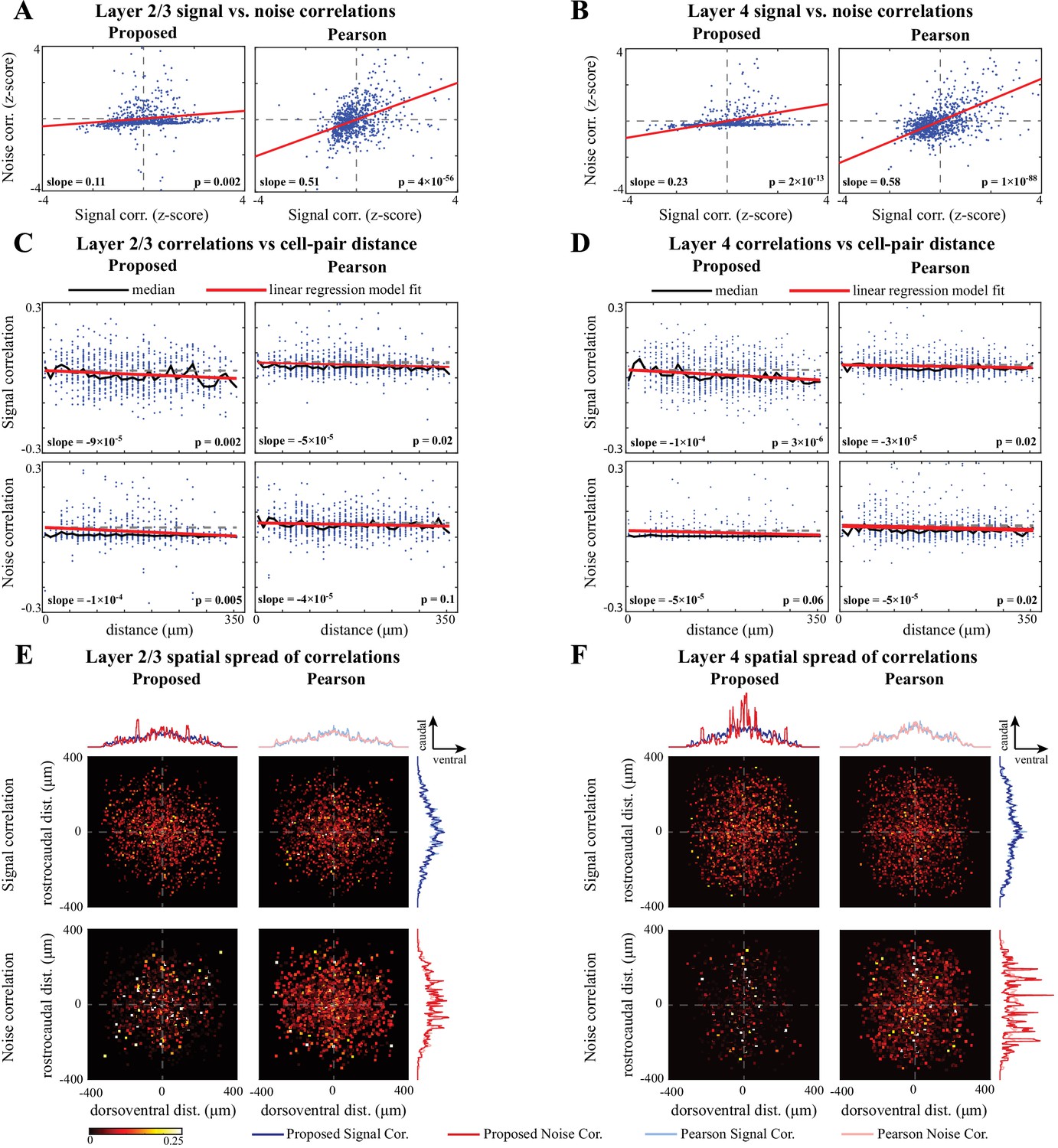
Comparison of signal and noise correlations across layers 2/3 and 4.

(A) Scatter-plot of noise vs. signal correlations (blue) for individual cell-pairs in layer 2/3, based on the proposed (left) and Pearson estimates (right). Data were normalized for comparison by computing z-scores. The linear model fits are shown in red, and the slope and p-value of the t-tests are indicated as insets. Panel (B) corresponds to layer 4 in the same organization as panel A. (C) Signal (top) and noise (bottom) correlations vs. cell-pair distance in layer 2/3, based on the proposed (left) and Pearson estimates (right). Distances were binned to $10 μ m$ intervals. The median of the distributions (black) and the linear model fit (red) are shown in each panel. The slope of the linear model fit, and the p-value of the t-test are also indicated as insets. Dashed horizontal lines indicate the zero-slope line for ease of visual comparison. Panel D corresponds to layer 4 in the same organization as panel C. (E) Spatial spread of signal (top) and noise (bottom) correlations in layer 2/3, based on the proposed (left) and Pearson estimates (right). The horizontal and vertical axes in each panel respectively represent the relative dorsoventral and rostrocaudal distances between each cell-pair, and the heat-map indicates the magnitude of correlations. Marginal distributions of the signal (blue) and noise (red) correlations along the dorsoventral and rostrocaudal axes for the proposed method (darker colors) and Pearson method (lighter colors) are shown at the top and right sides of the sub-panels. Panel F corresponds to layer 4 in the same organization as panel E.

Figure 7—figure supplement 1

Download asset Open asset

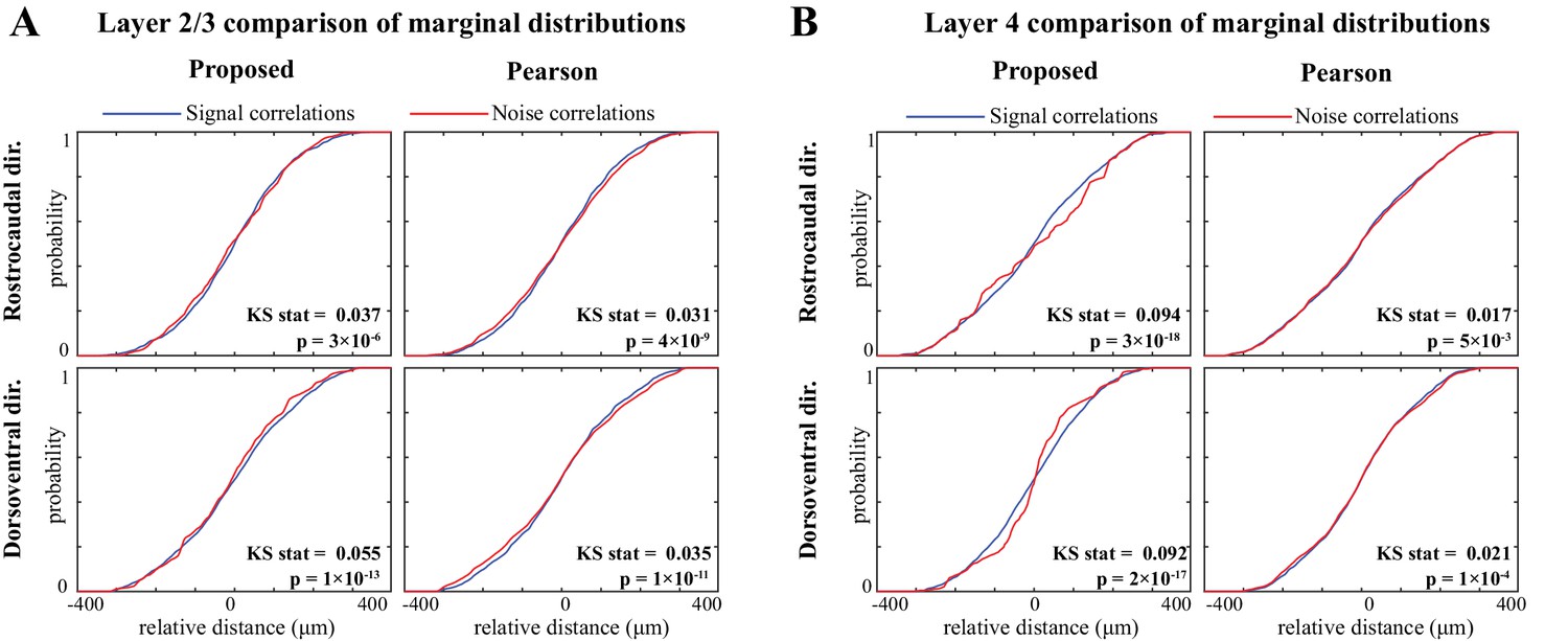
Comparing the marginal distributions of signal and noise correlations along the dorsoventral and rostrocaudal axes.

Comparison of marginal distributions of signal and noise correlations. (A) Cumulative marginal probability distributions of signal (blue) and noise (red) correlations along the rostrocaudal (top) and dorsoventral (bottom) directions, as estimated by the proposed method (left) and Pearson correlations from two-photon data (right), in layer 2/3 neurons. The Kolmogorovâ€“Smirnov (KS) test statistic along with the corresponding p-values are indicated as insets in each panel. Panel B shows the results for layer 4 in the same organization as panel A. These results show that along both directions and in both layers, the signal correlation distributions are significantly different from the corresponding noise correlation distributions, consistently for both methods. However, the KS statistics (i.e. effect sizes) for the proposed estimate are remarkably larger than those obtained from the Pearson estimates.

Figure 7—figure supplement 2

Download asset Open asset

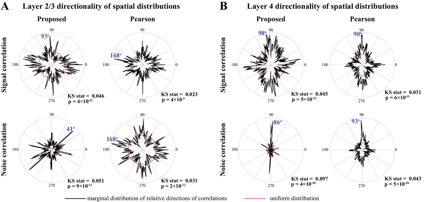
Marginal angular distributions of signal and noise correlations.

Polar plots of the angular marginal distributions of correlations. (A) Polar histograms indicating the distribution of signal (top) and noise (bottom) correlations as a function of relative angle (in the dorsoventral-rostrocaudal coordinate system) between pairs of neurons in layer 2/3, as estimated by the proposed method (left) and Pearson correlations from two-photon data (right). The KS test statistic comparing each polar distribution with a uniform distribution (shown in magenta), along with the corresponding p-values are indicated below each polar plot. The mode of each probability distribution is also indicated in blue fonts. Panel B shows the results for layer four in the same organization as panel A. All distributions are significantly non-uniform, and particularly indicate a rostrocaudal directionality in layer 4 (as indicated by the mode angles in panel B).

Figure 8

Download asset Open asset

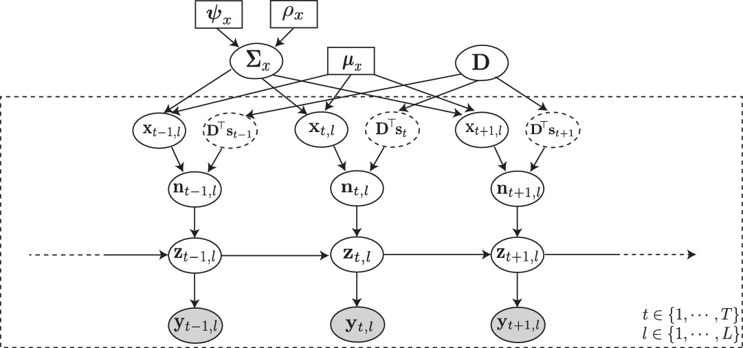
Probabilistic graphical model of the proposed forward model.

The fluorescence observations at the $t^{𝗍𝗁}$ time frame and $l^{𝗍𝗁}$ trial: $𝐲_{t, l}$ , are noisy surrogates of the intracellular calcium concentrations: $𝐳_{t, l}$ . The calcium concentration at time $t$ is a function of the spiking activity $𝐧_{t, l}$ , and the calcium activity at the previous time point $𝐳_{t - 1, l}$ . The spiking activity is driven by two independent mechanisms: latent trial-dependent covariates $𝐱_{t, l}$ , and contributions from the known external stimulus $𝐬_{t}$ , which we model by $𝐃^{⊤} 𝐬_{t}$ (in which the receptive field $𝐃$ is unknown). Then, we model $𝐱_{t, l}$ as a Gaussian process with constant mean $𝝁_{x}$ , and unknown covariance $𝚺_{x}$ . Finally, we assume the covariance $𝚺_{x}$ to have an inverse Wishart prior distribution with hyper-parameters $ψ_{x}$ and $ρ_{x}$ . Based on this forward model, the inverse problem amounts to recovering the signal and noise correlations by directly estimating $𝚺_{x}$ and $𝐃$ (top layer) from the fluorescence observations ${𝐲_{t, l}}_{t = 1, l = 1}^{T, L}$ (bottom layer).

Tables

Table 1

Dissimilarity metric statistics for the estimates in Figure 4A (also illustrated in Figure 4D), linear regression statistics of the comparison between signal and noise correlations in Figure 4E, and the average NMSE across 50 trials used in the shuffling procedure illustrated in Figure 5A.

	Dissimilarity $T_{d} (\hat{𝐒}, \hat{𝐍})$	Regression statistics (Figure 4E)		Shuffling test (Figure 5)
Estimate	Figure 4D	Slope (p-value)	$R^{2}$ Value	NMSE in $\hat{𝐍}$	NMSE in $\hat{𝐒}$
Proposed	$0.8725 (p < 10^{- 4})$	$0.02 (p = 0.84)$	$4 \times 10^{- 4}$	$1.07 \pm 0.16$	$1.32 \pm 0.19$
Pearson	$0.6675 (p = 0.71)$	$0.33 (p = 2 \times 10^{- 4})$	0.11	0	0
Two-stage Pearson	$0.7325 (p = 0.09)$	$0.15 (p = 0.10)$	0.02	$1.84 \pm 0.34$	$0.55 \pm 0.12$
Two-stage GPFA	$0.7625 (p < 10^{- 4})$	$0.02 (p = 0.86)$	$3 \times 10^{- 4}$	$2.32 \pm 0.52$	$2.26 \pm 0.51$

Table 2

Similarity/dissimilarity metric statistics for the estimates in Figure 6.

Estimation method	$T_{s} ({\hat{𝐍}}_{𝗌𝗉𝗈𝗇}, {\hat{𝐍}}_{𝗌𝗍𝗂𝗆})$	$T_{d} ({\hat{𝐒}}_{𝗌𝗍𝗂𝗆}, {\hat{𝐍}}_{𝗌𝗍𝗂𝗆})$
Proposed	0.5716 ( $p = 0.003$ )	0.7946 ( $p = 0.004$ )
Pearson	0.3031 ( $p = 0.61$ )	0.5032 ( $p = 0.92$ )
Two-stage Pearson	0.2790 ( $p = 0.05$ )	0.7862 ( $p = 0.39$ )
Two-stage GPFA	0.2008 ( $p = 0.50$ )	0.7792 ( $p = 0.22$ )

Table 3

Linear regression statistics for the analysis of correlations vs. cell-pair distance.

	Statistics of layer 2/3 correlations		Statistics of layer 4 correlations
Correlations	Slope (p-value)	$R^{2}$ Value	Slope (p-value)	$R^{2}$ Value
Proposed Signal Corr.	$- 𝟗 \times {𝟏𝟎}^{- 𝟓}$ ( $p = 0.002$ )	0.012	$- 𝟏 \times {𝟏𝟎}^{- 𝟒}$ ( $p = 3 \times 10^{- 6}$ )	0.023
Pearson Signal Corr.	$- 5 \times 10^{- 5}$ ( $p = 0.02$ )	0.007	$- 3 \times 10^{- 5}$ ( $p = 0.02$ )	0.005
Proposed Noise Corr.	$- 𝟏 \times {𝟏𝟎}^{- 𝟒}$ ( $p = 0.005$ )	0.010	$- 𝟓 \times {𝟏𝟎}^{- 𝟓}$ ( $p = 0.06$ )	0.004
Pearson Noise Corr.	$- 4 \times 10^{- 5}$ ( $p = 0.1$ )	0.003	$- 5 \times 10^{- 5}$ ( $p = 0.02$ )	0.005

Additional files

Transparent reporting form: https://cdn.elifesciences.org/articles/68046/elife-68046-transrepform-v2.docx
Download elife-68046-transrepform-v2.docx

Download links

A two-part list of links to download the article, or parts of the article, in various formats.

Downloads (link to download the article as PDF)

Open citations (links to open the citations from this article in various online reference manager services)

Mendeley

Cite this article (links to download the citations from this article in formats compatible with various reference manager tools)

Anuththara Rupasinghe
Nikolas Francis
Ji Liu
Zac Bowen
Patrick O Kanold
Behtash Babadi

(2021)

Direct extraction of signal and noise correlations from two-photon calcium imaging of ensemble neuronal activity

eLife 10:e68046.

https://doi.org/10.7554/eLife.68046

Share this article

Cite this article

The proposed generative model and inverse problem.

Results of simulation study 1.

Sensitivity of two-stage estimates to the choice of the underlying spike deconvolution technique.

Performance of two-stage estimates based on ground truth spikes.

Performance comparison under stimulus integration model mismatch.

Performance under calcium decay model mismatch.

Performance comparison under varying SNR levels and firing rates.

Performance comparison under observation noise model mismatch.

Results of simulation study 2.

Application to experimentally-recorded data from the mouse A1.

Probing the effect of stimulus integration window length on the performance of the proposed estimates.

Inspecting the inferred latent processes under high fluorescence activity due to rapid increase in firing rate.

Assessing the specificity of different estimation results shown in Figure 4.

Comparison of spontaneous and stimulus-driven activity in the mouse A1.

Histograms of the similarity/dissimilarity metrics under the shuffling procedure.

Comparison of signal and noise correlations across layers 2/3 and 4.

Comparing the marginal distributions of signal and noise correlations along the dorsoventral and rostrocaudal axes.

Marginal angular distributions of signal and noise correlations.

Probabilistic graphical model of the proposed forward model.

Dissimilarity metric statistics for the estimates in Figure 4A (also illustrated in Figure 4D), linear regression statistics of the comparison between signal and noise correlations in Figure 4E, and the average NMSE across 50 trials used in the shuffling procedure illustrated in Figure 5A.

Similarity/dissimilarity metric statistics for the estimates in Figure 6.

Linear regression statistics for the analysis of correlations vs. cell-pair distance.

Transparent reporting form

Downloads (link to download the article as PDF)

Open citations (links to open the citations from this article in various online reference manager services)

Cite this article (links to download the citations from this article in formats compatible with various reference manager tools)