3D cell neighbour dynamics in growing pseudostratified epithelia
- Department of Biosystems Science and Engineering (D-BSSE), ETH Zürich, Switzerland
- Swiss Institute of Bioinformatics (SIB), Switzerland
Figures
Figure 1
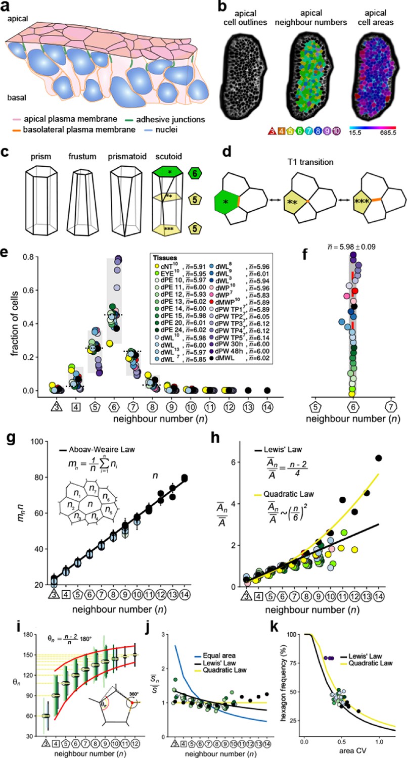
Principles of epithelial organisation.
(a) Schematic representation of an epithelial tissue layer. The cells are polarised between an apical and a basal side. Near the apical side, cells adhere tightly via adhesion junctions (green). Nuclei are depicted in blue. (b) Apical surface projection of an embryonic lung bud at E12.5 imaged using light-sheet microscopy. Cell contour segmentations (left) coloured according to neighbour relationships (middle) and area quantifications (right). (c) Current shape representations of 3D epithelial cells: prism, frustum, prismatoid, and scutoid. (d) Planar cell neighbour exchange (T1 transition). (e) Tissues differ widely in the frequency of neighbour numbers. The legend provides the measured average number of cell neighbours for each tissue and the references to the primary data (Classen et al., 2005; Escudero et al., 2011; Etournay et al., 2015; Farhadifar et al., 2007; Gibson et al., 2006; Heller et al., 2016; Sánchez-Gutiérrez et al., 2016). Data points for n < 3 were removed as they must present segmentation artefacts. (f) The measured average number of cell neighbours is close to the topological requirement () in all tissues; see panel e for the colour code. (g) Epithelial tissues follow the AW law (black line). The AW law formulates a relationship between the average number of neighbours, n, that a cell has and that its direct neighbours have, . The product can be determined by summing over all ni. (h) The relative average apical cell area, , increases with the number of neighbours, n, and mostly follows the linear Lewis’ law (Equation 2, black line), or the quadratic relationship (Equation 3, yellow line) in case of higher apical area variability. (i) The average internal angle by polygon type is close to that of a regular polygon, (yellow lines). To form a contiguous lattice, the angles at each tricellular junction must add to 360°, and the resulting observed deviation in the angles follows the prediction (red line). (j) The average normalised side length by polygon type. (k) Observed fraction of hexagons versus area coefficient of variation (CV). The curves mark theoretical predictions when polygonal cell layers follow either the linear Lewis’ law (Equation 2, black line) or the quadratic law (Equation 3, yellow line). The colour code in panels g-k is as in panel e, but data is available only for a subset of tissues. The abbreviations in panel (e) are as follows: cNT refers to the Chick neural tube epithelium, EYE to the Drosophila eye disc, dPE to the Drosophila peripodal membrane from the larval eye disc, dWL to the Drosophila larval wing disc, dWP to the Drosophila pre-pupal wing disc, dMWP to the Drosophila mutant wing pre-pupa with reduced expression of myosin II, dPW to the Drosophila pupal wing disc, and dMWL to the wing disc with gigas RNAi clones. TPx indicates subsequent but not further specified pupal time points.
© 2019, Kokic et al. Panels e, f, g and k are reproduced with modifications from Figures 1,5 from Kokic et al., 2019, which are published under the Creative Commons Attribution Non-Commercial 4.0 International License
© 2019, Vetter et al. Panels g and i are reproduced with modifications from Figures 1,5 from Vetter et al., 2019, which are published under the Creative Commons Attribution Non-Commercial 4.0 International License
Figure 2 with 4 supplements
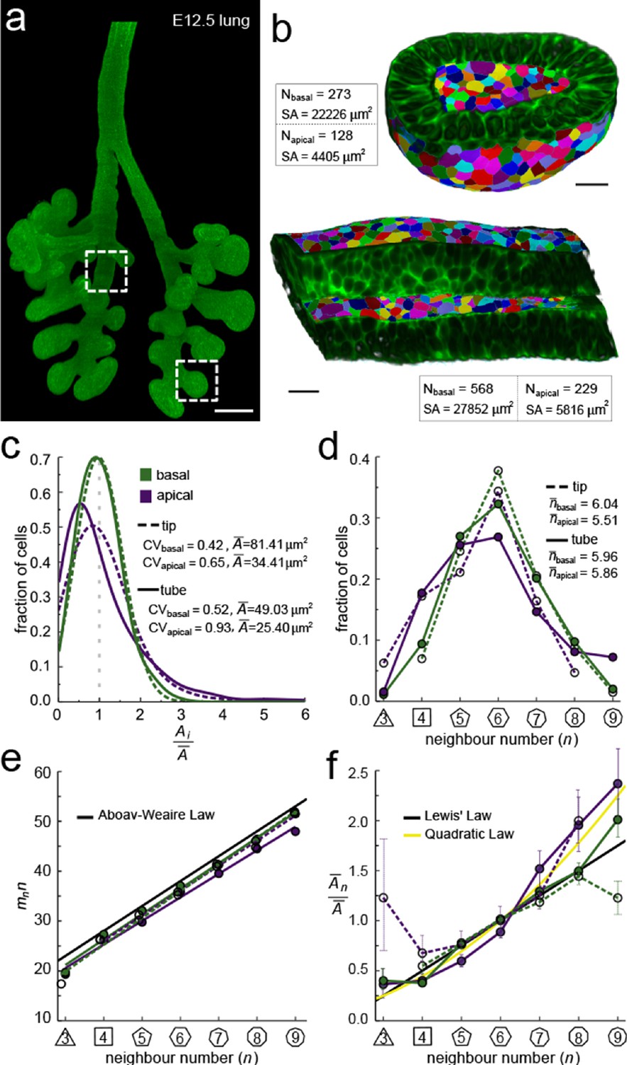
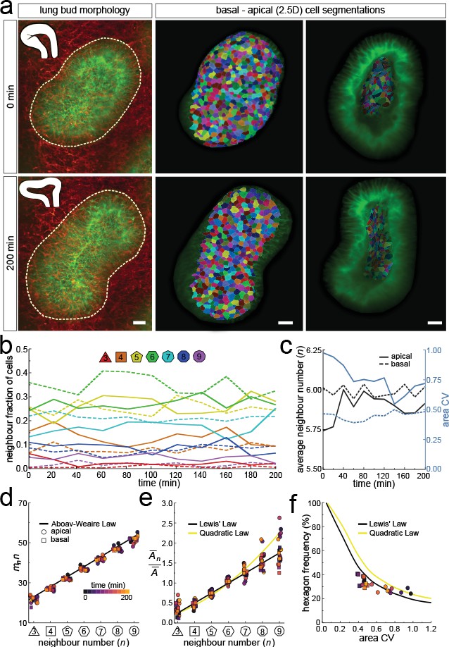
Apical and basal epithelial organisation.
(a) Epithelium of E12.5 ShhGC/+; ROSAmT/mG mouse embryonic lung imaged using light-sheet microscopy. Scale bar 200 µm. Corresponding 2D sections are shown in Figure 2—figure supplement 1, and Figure 2—video 1. (b) Apical and basal 2.5D cell segmentation overlays on imaged tip and tube sections (dotted boxes in panel a). An illustration of the 2.5D segmentation workflow is presented in Figure 2—figure supplement 2. Number of cells (N) and segmented surface areas (SA) are given. Cells are coloured using random labels. Scale bars 20 µm. (c) Normalised apical and basal cell area distributions in the tip (broken lines) and tube (solid lines) datasets. The colour code in panel c is reused in panels d-f. (d) Frequencies of neighbour numbers on the apical and basal sides in the tip and tube datasets. (e) The apical and basal layers follow the AW law (black line). SEM is smaller than symbols. (f) The normalised average cell area, , increases with the number of neighbours, n. The basal cells (green) follow Lewis’ law (Equation 2, black line), while the apical cells (purple) follow the quadratic relationship (Equation 3, yellow line). SEM as error bars.
-
Figure 2—source data 1
2.5D neighbour number and area data.
- https://cdn.elifesciences.org/articles/68135/elife-68135-fig2-data1-v2.xls
-
Figure 2—source data 2
2.5D AW data.
- https://cdn.elifesciences.org/articles/68135/elife-68135-fig2-data2-v2.xls
Figure 2—figure supplement 1
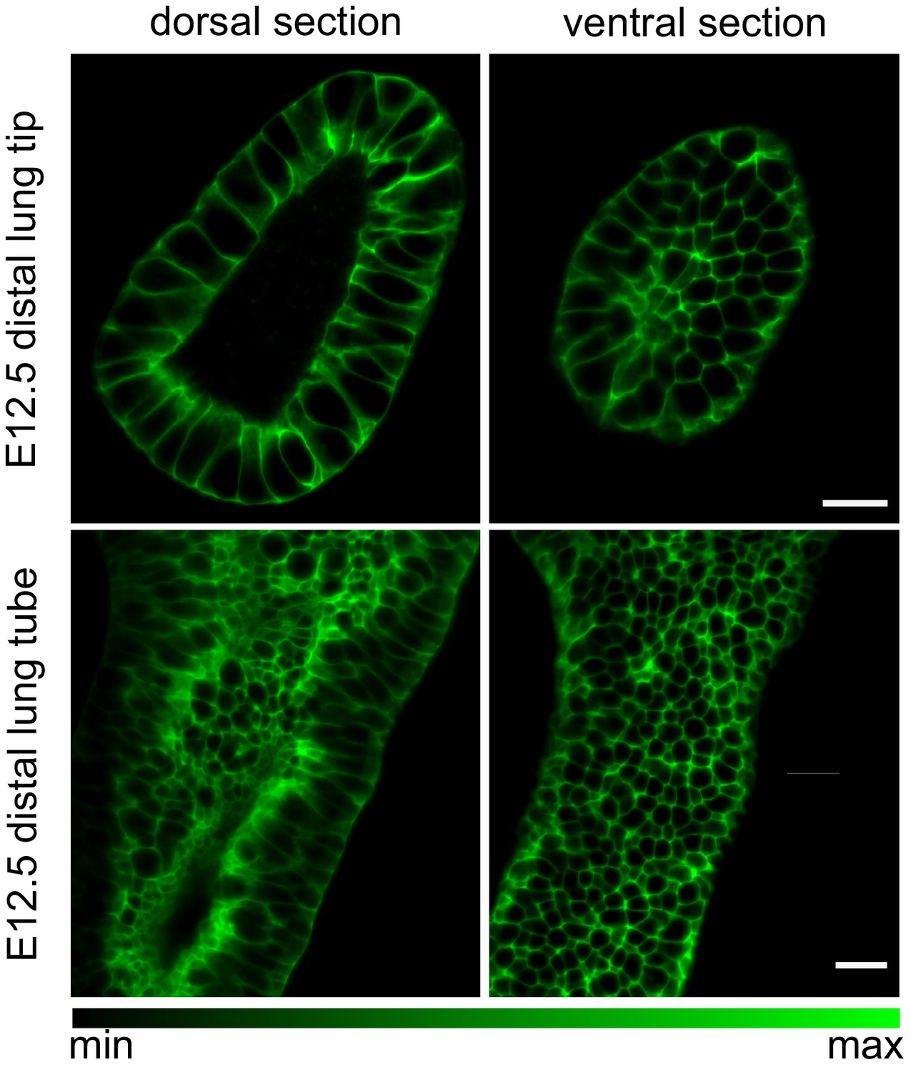
Embryonic mouse lung rudiments.
Dorsal and ventral cross-sections of an E12.5 lung tip and tube carrying the ShhGC/+; ROSAmT/mG reporter allele, marking the epithelial lineage. Tissue explants were optically cleared using CUBIC and imaged using light-sheet microscopy to achieve cellular resolution at all depths. Scale bars 20 µm.
Figure 2—figure supplement 2
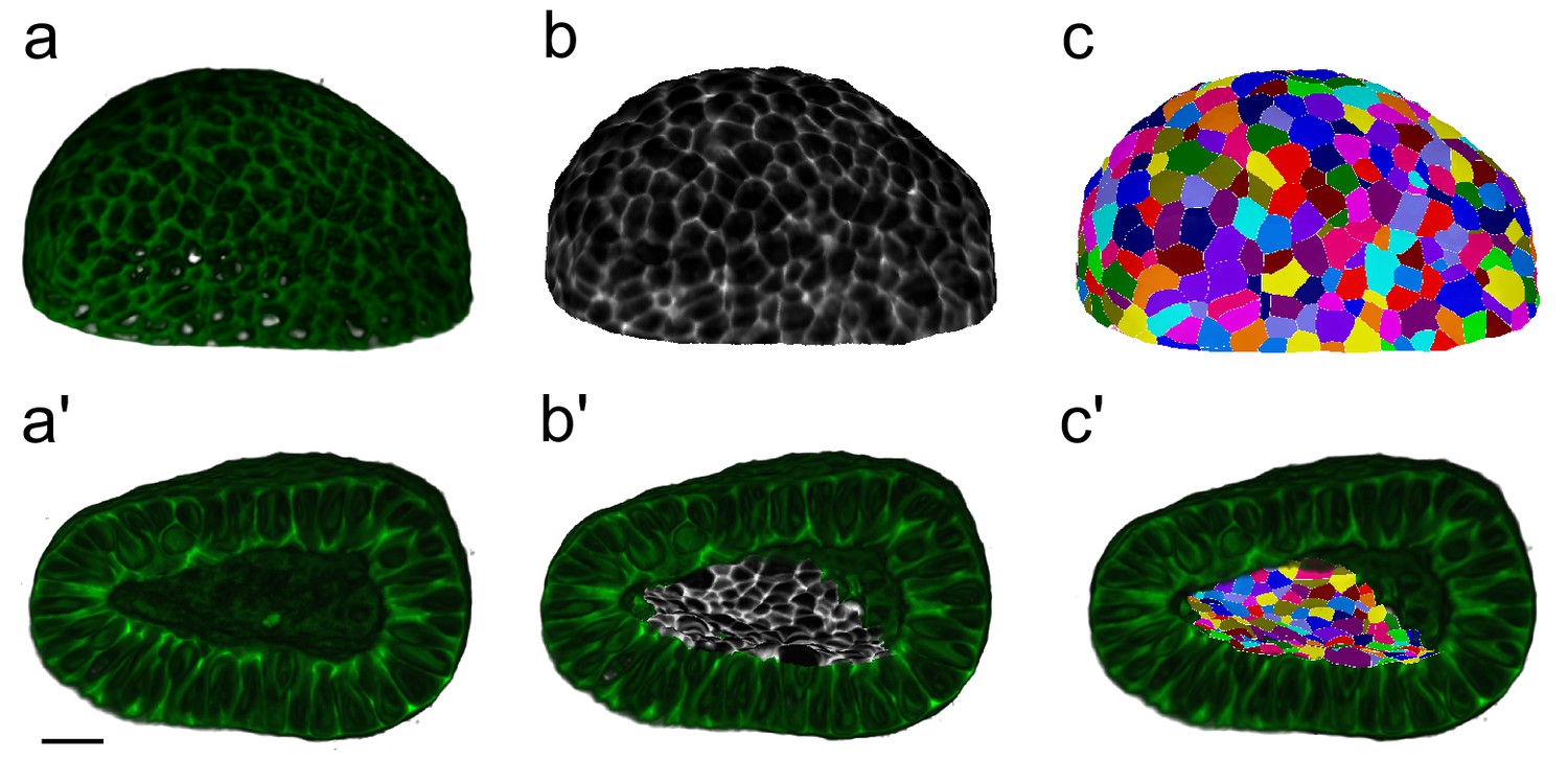
Workflow for surface cell segmentations.
MorphoGraphX segmentation workflow to extract cell segmentations along curved surface boundaries (2.5D) for a CUBIC-cleared murine E12.5 distal lung tip. The illustrated sample expressed the ShhGC/+; ROSAmT/mG reporter and was imaged using light-sheet microscopy. (a–c) Correspond to the basal layer while (a’–c') correspond to the apical domain. (a, a’) Deconvolved light-sheet microscopy 3D renderings showing the basal and apical surfaces. (b, b') Curved surfaces are isolated, meshed, and the adjacent fluorescent signal is projected. (c, c') Apical and basal domains are segmented (2.5D segmentations) and coloured by random label numbers. Scale bar 20 µm.
Figure 2—figure supplement 3

CUBIC clearing of embryonic tissue.
Protocol for advanced CUBIC (Clear, Unobstructed Brain/Body Imaging Cocktails and Computational analysis) of a murine lung rudiment (Susaki et al., 2015). Serial dilutions in reagent-1 and reagent-2 guarantee that morphology is not distorted and that optical transparency is achieved within 1 week with high reproducibility.
Figure 2—video 1
Optically cleared mouse lung rudiment image stacks.
Animated cross-section exploration of murine E12.5 lung tip and tube image stacks. Specimens carried the ShhGC/+; ROSAmT/mG reporter allele to mark the epithelial lineage were CUBIC cleared, and subsequently imaged using light-sheet microscopy to achieve cellular resolution. Scale bars 20 µm. (AVI 83.1 MB).
Figure 3 with 4 supplements
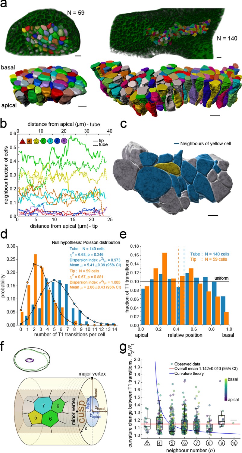
3D epithelial organisation.
(a) 3D iso-surfaces of segmented epithelial tip (N=59) and tube (N=140) cells from a ShhGC/+; ROSAmT/mG E12.5 mouse lung rudiment imaged using light-sheet microscopy. Morphometric quantifications of cell boundary segmentations along the apical-basal axis were used to study spatial T1 transitions. The 3D segmentation workflow is introduced in Figure 3—figure supplement 1 and Figure 3—videos 1–3 illustrate the rendered epithelial tip, tube and all segmented volumes. Scale bars 10 µm. (b) Frequency of neighbour numbers as quantified along the apical basal axis in the tip (solid lines) and tube (broken lines) datasets. (c) Extent of neighbour contacts (center cell in yellow and neighbours in blue) in 3D as viewed from the apical side. Scale bars 5 µm. (d) Probability distributions of the lateral T1 transitions for tip (total=169, mean=2.86, N=59) and trunk (total=746, mean=5.41, N=140) datasets are consistent with Poisson distributions. (e) Normalised apical-basal distribution of T1 transitions for all cells shows no apical-basal bias, except for fewer transitions close to the basal surface. (f). Schematic of a tubular epithelium with elliptic cross section. The analysed cells are located in the cusp (brown) of the tube, where the local tissue curvature is close to that of the minor ellipse vertex. Subpanel illustrates ellipse fitting to apical (purple) and basal (green) domain boundaries. Lighter outlines correspond to the most proximal segment of the tube in Figure 2b, while darker ones to the most distal section. (g) The predicted impact of a curvature effect on T1 transitions decreases with increasing cell neighbour numbers (blue line). The measured T1 transitions for different neighbour numbers do not support a curvature effect (dots, boxplots, and red line). Boxplots indicate the median, 25% and 75% percentiles of the data.
-
Figure 3—source data 1
3D neighbour number and area data.
- https://cdn.elifesciences.org/articles/68135/elife-68135-fig3-data1-v2.xls
-
Figure 3—source data 2
3D curvature change data.
- https://cdn.elifesciences.org/articles/68135/elife-68135-fig3-data2-v2.xls
Figure 3—figure supplement 1
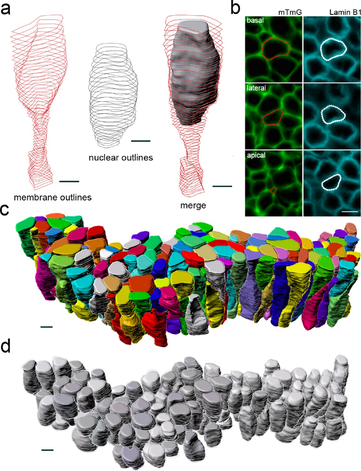
Workflow for 3D epithelial cell and nuclear segmentations.
Segmentation workflow to extract cellular and nuclear 3D shapes from a CUBIC-cleared murine E12.5 lung tube. The specimen used expressed the ShhGC/+; ROSAmT/mG reporter and was immunostained for lamin B1 to both selectively label cell membranes and mark nuclear envelopes. Light-sheet microscopy was used. (a) Sequential contour surfaces are drawn to follow cell membrane and nuclear outlines on a number of planes along the apical-basal axis. By interpolating between contours, iso-surfaces accurately representing 3D shapes can be extracted. (b) Membrane and nuclear contour surface overlays at different tissue depths. (c) Extracted 3D cell, and (d) nuclear iso-surfaces (N=140) for developing mouse lung. Co-planar contours were used for morphometric quantifications. All scale bars 5 µm.
Figure 3—video 1
3D contour surfaces.
Image stack animation illustrating nuclear and cell contour surface overlays (left, middle) along the apical-basal axis as well as full 3D iso-surfaces (right) for a single cell. A CUBIC-cleared E12.5 ShhGC/+; ROSAmT/mG lung tube showing epithelial membranes in green was immunostained for lamin B1 rendering nuclear envelopes blue. Scale bar 5 µm (AVI 11.8 MB).
Figure 3—video 2
3D nuclear and tube cell segmentations.
Volumetric rendering of an E12.5 ShhGC/+; ROSAmT/mG lung tube (green epithelia) imaged using light-sheet microscopy. 3D cellular and nuclear segmentations (N=140) were facilitated by CUBIC tissue clearing (AVI 42.0 MB).
Figure 3—video 3
3D tip cell segmentations.
Volumetric rendering of an E12.5 ShhGC/+; ROSAmT/mG lung tip (green epithelia) imaged using light-sheet microscopy. 3D cellular segmentations (N=59) were facilitated by CUBIC tissue clearing (AVI 12.4 MB).
Figure 4
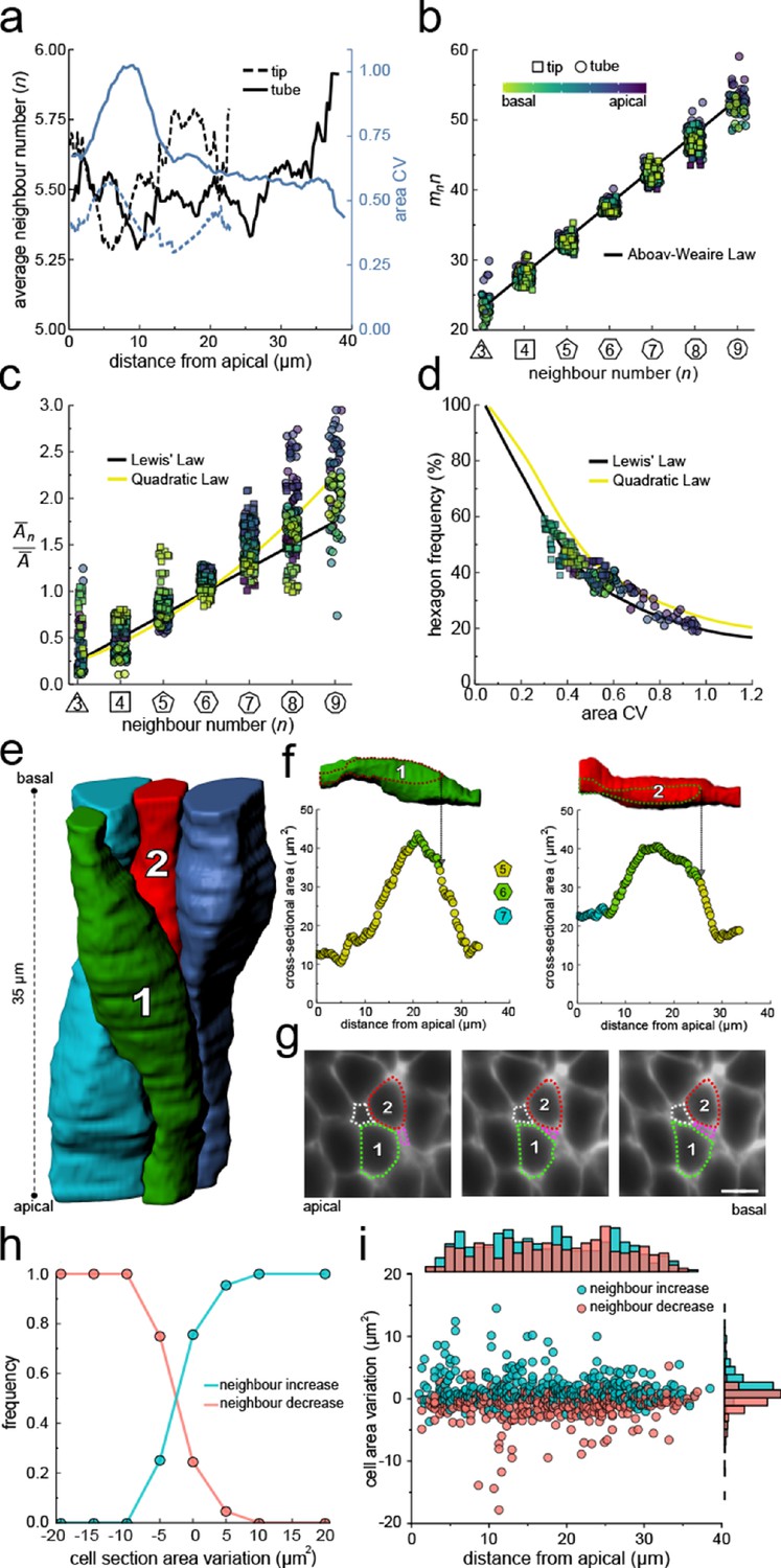
Neighbour changes along the apical-basal axis are driven by changes in cross-sectional area.
(a) Average number of neighbours (black) and area CV (blue) along the apical basal axis in the tip and tube datasets. (b) All epithelial layers follow the AW law (black line). The colour code in panels c, d follow that in panel b. (c) All epithelial layers follow Lewis’ law (Equation 2, black line) in case of low, and the quadratic relationship (Equation 3, yellow line) in case of high cell area variability. (d) Observed fraction of hexagons versus area CV for segmented cell layers along the apical-basal axis. The lines mark the theoretical prediction if polygonal cell layers follow either the linear Lewis’ law (black line) or the quadratic law (yellow line). (e) 3D iso-surfaces of four segmented epithelial cells in a CUBIC-cleared ShhGC/+; ROSAmT/mG E12.5 distal lung tube, with 140 3D segmented epithelial cells (Figure 3—figure supplement 1c). (f) Cross-sectional area and cell neighbour number along the apical-basal axis for marked cells in panel e. Dotted lines indicate contact with one another. (g) Lateral cross-sections illustrating a T1 transition along the apical-basal axis (0.664 µm in-between frames). Scale bar 6 µm. (h) An increase in the cell cross-sectional area increases the frequency of a neighbour number increasing spatial T1 transitions, and vice versa. (i) Apical-basal distribution of spatial T1 transitions according to neighbour increase or decrease and cross-sectional area variation.
-
Figure 4—source data 1
3D area CV and avg. neighbour number data.
- https://cdn.elifesciences.org/articles/68135/elife-68135-fig4-data1-v2.xls
-
Figure 4—source data 2
3D AW data.
- https://cdn.elifesciences.org/articles/68135/elife-68135-fig4-data2-v2.xls
-
Figure 4—source data 3
Neighbour exchange/type data.
- https://cdn.elifesciences.org/articles/68135/elife-68135-fig4-data3-v2.xls
Figure 5 with 2 supplements

Changes in cross-sectional area as a result of interkinetic nuclear migration (IKNM).
(a) Light-sheet microscopy longitudinal sections of an E12.5 CUBIC-cleared lung tube carrying the ShhGC/+; ROSAmT/mG reporter allele (green epithelium) and immunostained for lamin B1 (blue nuclear envelopes). Morphometric quantifications of 3D iso-surfaces (N=140) and cell segmentations along the apical-basal axis were used to study the nature of cross-sectional area variation and the effect of IKNM (Figure 3—figure supplement 1). Scale bar 20 µm. (b) Sequential cell membrane contour surfaces and nuclear iso-surfaces for six epithelial cells. By interpolating between contours and creating iso-surfaces, 3D shapes can be accurately extracted (Figure 3—video 2 and Figure 5—video 1). Scale bar 7 µm. (c) Distribution of nuclei center of mass along the apical-basal axis. (d) Nuclear ellipticity and volume distributions along the apical-basal axis. (e) Average cross-sectional area distribution along the apical-basal axis for all cells (black) and nuclei (blue). (f). Nuclear and cellular volumes of 140 segmented cells are correlated (r=0.79). Line of best fit in red. (g). The cell and corresponding nuclear cross-sectional areas along the apical-basal axis are highly correlated (r=0.94). (h). Diameters of nuclei and cells based on the measured nuclear and cell volumes if nuclei were perfect spheres, and cells were perfect cylinders of the measured height. Given the larger nuclear diameter, nuclei must deform in order to fit within cells. (i) An increase in the nuclear cross-sectional area increases the frequency of a neighbour-number-increasing spatial T1 transitions, and vice versa. (j) The largest number of changes in neighbour relationships occur at the apical and basal limits of the nucleus for all cells, where cross-sectional areas change sharply.
-
Figure 5—source data 1
3D neighbour number, cell area, and nuclear area data.
- https://cdn.elifesciences.org/articles/68135/elife-68135-fig5-data1-v2.xls
-
Figure 5—source data 2
Volume and ellipticity data.
- https://cdn.elifesciences.org/articles/68135/elife-68135-fig5-data2-v2.xls
-
Figure 5—source data 3
3D cell and nuclear diameter data.
- https://cdn.elifesciences.org/articles/68135/elife-68135-fig5-data3-v2.xls
Figure 5—figure supplement 1
Light-sheet imaging of a stained embryonic mouse lung rudiment.
Volumetric renderings and orthogonal projections obtained from light-sheet microscopy for an E12.5 embryonic lung. The above specimen carried the ShhGC/+;ROSAmT/mG to mark (a) epithelial cell membranes and was (b) immunostained for lamin B1 to mark nuclear envelopes. (c) Merged fluorescent signal. Scale bar 20 µm.
Figure 5—video 1
3D nuclear iso-surface segmentations and cell membrane contours.
Volumetric rendering of sequential cell membrane contour surfaces and nuclear iso-surfaces from an E12.5 ShhGC/+; ROSAmT/mG lung tube immunostained for lamin B1. The sample was cleared using CUBIC and imaged on a Z.1 Zeiss light-sheet microscope (AVI 8.70 MB).
Figure 6 with 4 supplements
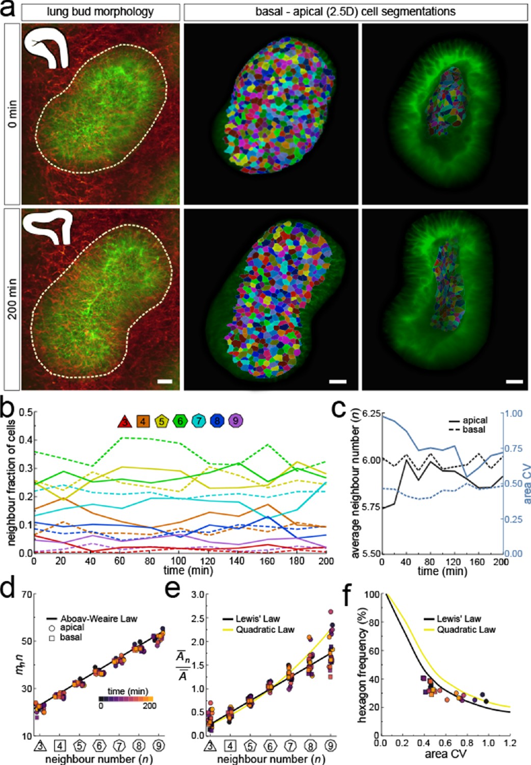
Dynamics of apical and basal epithelial organisation.
(a) Timelapse light-sheet microscopy series of a cultured mouse E12.5 distal lung bud expressing the ShhGC/+; ROSAmT/mG reporter (green epithelium, and red mesenchyme), imaged every 20 min (11 time steps). The white inset denotes the morphology of the lung bud, while the dotted area denotes the segmented cell patch. Corresponding visual provided in Figure 6—video 1. Cells on both the apical and basal domains were 2.5D segmented, and their morphology quantified. Corresponding visual provided in Figure 6—video 3. Scale bars 20 µm. (b) Cell neighbour frequencies for the apical and basal layers over time. (c) Observed average neighbour number and area coefficient of variation (CV) for the apical and basal layers over time. (d) Growing apical and basal layers follow the AW law (black line). Colour code applies to e-f. (e) The relative average apical and basal cell areas are linearly related to the number of neighbours (in all time points) and follow Lewis’ law (black line), or the quadratic relationship in the case of higher area variability (yellow line). (f) Observed fraction of hexagons versus area coefficient of variation (CV) on the apical and basal layers. The lines mark the theoretical prediction if polygonal cell layers follow either the linear Lewis’ law (black line) or the quadratic law (yellow line).
-
Figure 6—source data 1
2.5D neighbour number and area data over time.
- https://cdn.elifesciences.org/articles/68135/elife-68135-fig6-data1-v2.xls
-
Figure 6—source data 2
2.5D area CV and avg. neighbour number data over time.
- https://cdn.elifesciences.org/articles/68135/elife-68135-fig6-data2-v2.xls
-
Figure 6—source data 3
2.5D AW data over time.
- https://cdn.elifesciences.org/articles/68135/elife-68135-fig6-data3-v2.xls
Figure 6—figure supplement 1
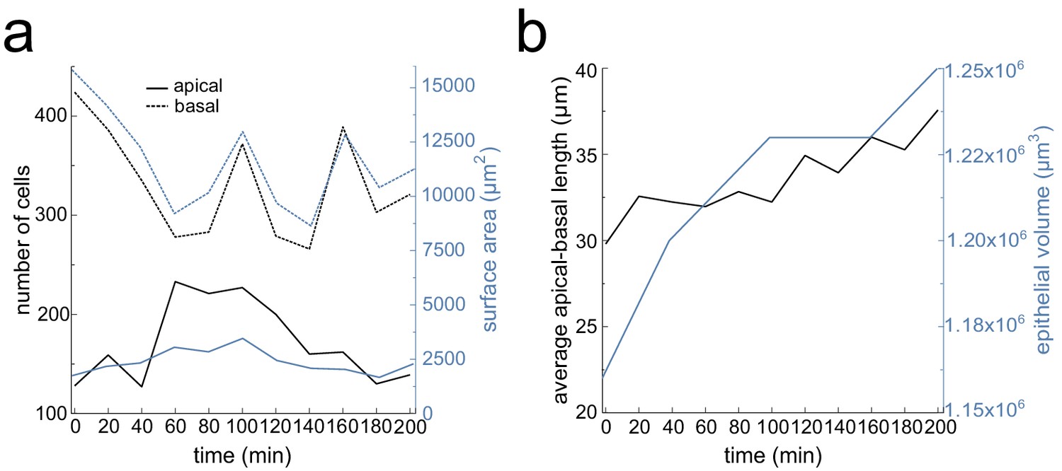
Lung bud viability and growth quantifications over time.
(a) Number of segmented cells and surface area for the apical and basal layers over time. (b) Average apical-basal length and epithelial volume over time. Tissue thickness was measured at five landmark regions along the growing bud.
Figure 6—video 1
High-resolution light-sheet microscopy timelapse imaging of epithelial lung development (10 hr).
Timelapse movie showing the development of an E12.5 mouse lung rudiment carrying the ShhGC/+; ROSAmT/mG construct. Embryonic lung was mounted in a hollow cylinder made from low-melting-point agarose and filled with matrigel to replicate the native microenvironment and promote near-physiological growth. Sample was imaged using the Zeiss Z.1 Lightsheet system for 10 hr, with frames acquired every 20 min. Top bud was used for quantifications (AVI 44.5 MB).
Figure 6—video 2
High-resolution light-sheet microscopy timelapse imaging of epithelial lung development (3 hr).
Timelapse movie showing the development of an E12.5 mouse lung rudiment carrying the ShhGC/+; ROSAmT/mG construct. Embryonic lung was mounted in a hollow cylinder made from low-melting-point agarose and filled with matrigel to replicate the native microenvironment and promote near-physiological growth. The sample was imaged using a Zeiss Z.1 Lightsheet, with frames acquired every 20 min. This subset includes all 11 time points (3 hr) used in Figure 6. Top bud was used for quantifications (AVI 59.2 MB).
Figure 6—video 3
Apical and basal surface cell segmentations.
Basal and apical cell segmentations overlays for a CUBIC-cleared E12.5 ShhGC/+; ROSAmT/mG mouse lung tip imaged using light-sheet microscopy every 20 min. MorphoGraphX was used to accurately extract curved surface meshes from 3D volumetric data. The resulting curved (2.5D) surface images of the apical and basal domains were segmented using the Watershed algorithm. Scale bar 20 µm (AVI 58.1 MB).
Figure 7 with 2 supplements
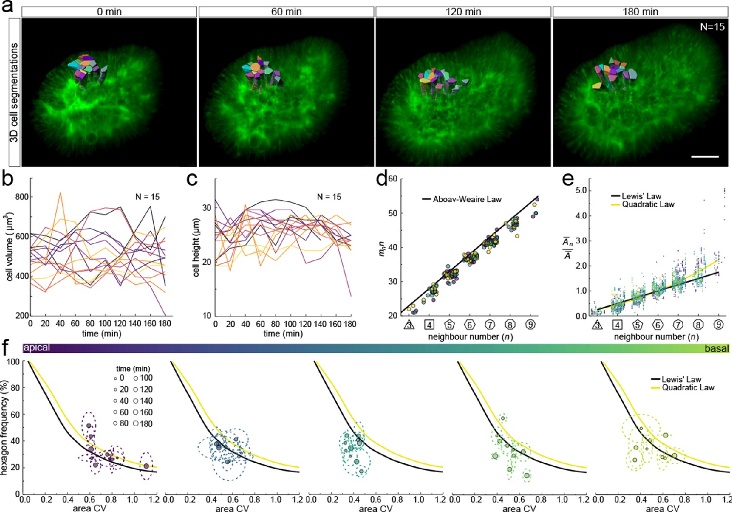
3D cell organisation in growing epithelia.
(a) 3D segmentation of 15 epithelial cells from timelapse light-sheet microscopy imaging of a mouse E12.5 distal lung bud expressing the ShhGC/+; ROSAmT/mG reporter. The specimen was imaged every 20 min over 3 hr. Planar segmentations along the apical-basal axis were pooled into five groups to enable morphometric analysis in different tissue regions. A full timelapse panel is provided in Figure 7—figure supplement 1 and Figure 7—video 1. Scale bar 30 µm. (b) Epithelial cell volume, and (c) height over time (N=15). (d) Segmented cells in pooled layers along the apical-basal axis follow the AW law (black line) over time (left to right); see panel f for colour code. (e) The relative average cell area in each layer is linearly related to the number of neighbours for all time points (left to right) and follows Lewis’ law (black line), or the quadratic relationship in the case of higher area variability (yellow line); see panel f for colour code. (f) Temporal dynamics of observed fraction of hexagons versus area coefficient of variation (CV) along the apical-basal axis. Dotted lines denote variation per time point. Solid lines mark the theoretical prediction if polygonal cell layers follow either the linear Lewis’ law (black line) or the quadratic law (yellow line).
-
Figure 7—source data 1
3D neighbour number and area data over time.
- https://cdn.elifesciences.org/articles/68135/elife-68135-fig7-data1-v2.xls
-
Figure 7—source data 2
3D area CV and hex percent data over time.
- https://cdn.elifesciences.org/articles/68135/elife-68135-fig7-data2-v2.xls
-
Figure 7—source data 3
3D AW data over time.
- https://cdn.elifesciences.org/articles/68135/elife-68135-fig7-data3-v2.xls
Figure 7—figure supplement 1
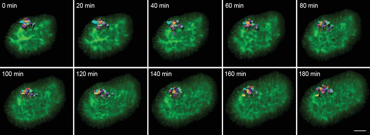
3D timelapse segmentation of growing epithelia.
Timelapse segmentation of growing epithelial cells from a CUBIC-cleared mouse E12.5 lung tip over 180 min; iso-surfaces coloured by cell identifier. The specimen used expressed the ShhGC/+; ROSAmT/mG reporter and was imaged using light-sheet microscopy. Scale bar 30 µm.
Figure 7—video 1
3D timelapse segmentation of growing epithelia.
Timelapse segmentation of growing epithelial cells from a CUBIC-cleared E12.5 mouse lung tube over 180 min, iso-surfaces coloured by cell identifier. This specimen expressed the ShhGC/+; ROSAmT/mG reporter and was imaged using light-sheet microscopy (AVI 9.45 MB).
Figure 8
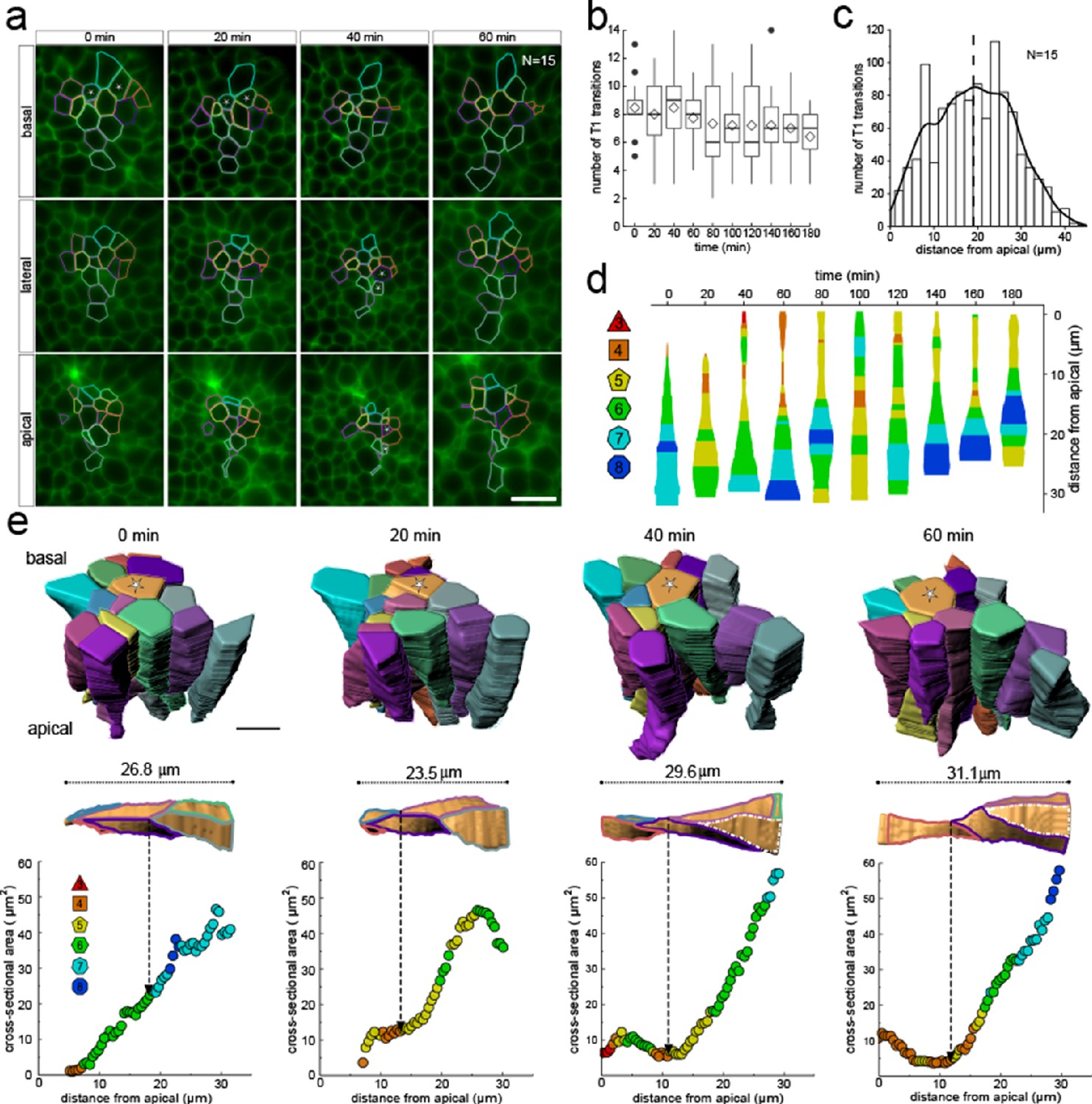
3D cell neighbour dynamics in growing epithelia.
(a) Apical, basal and lateral cross-sections from a light-sheet microscopy timelapse of a murine E12.5 distal lung bud expressing the ShhGC/+; ROSAmT/mG reporter. The specimen was imaged every 20 min over 3 hr. Cell membrane outlines illustrate fluid cell neighbour relationships along the apical-basal axis and over time. T1 transitions are marked with white stars; see panel e for cell colour code. Scale bar 14 µm. (b) Number of T1L transitions for all cells (N=15) over time. Diamonds represent the mean. Morphometric quantifications of planar segmentations along the apical-basal axis were used to examine T1L transition dynamics. (c) Spatial distribution along the apical-basal axis of T1L transitions for all cells and time points. (d) Temporal evolution of neighbour relationships along the apical-basal axis for a single cell. Schematic cell width corresponds to cross-sectional area. (e) (top row) 3D iso-surface segmentations of 15 epithelial cells. Scale bar 10 µm. (bottom row) Cross-sectional area and cell neighbour number along the apical-basal axis for a given cell (marked with a white star). Dotted lines indicate contact with a cell that was not segmented.
Appendix 1—figure 1
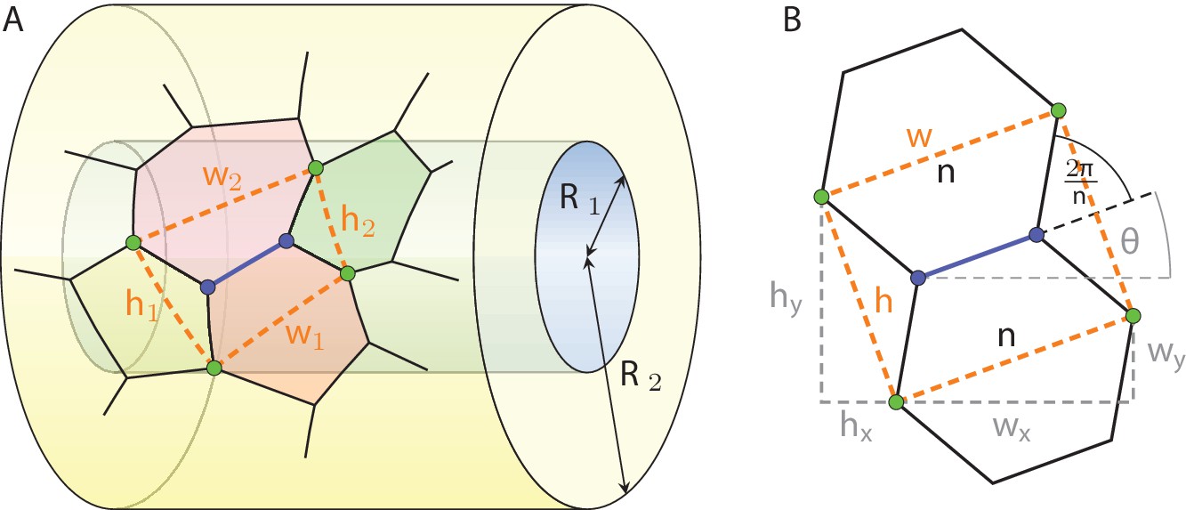
Definition of the vicinity of a cell edge in a geometric projection on a tubular epithelium.
Appendix 1—figure 2
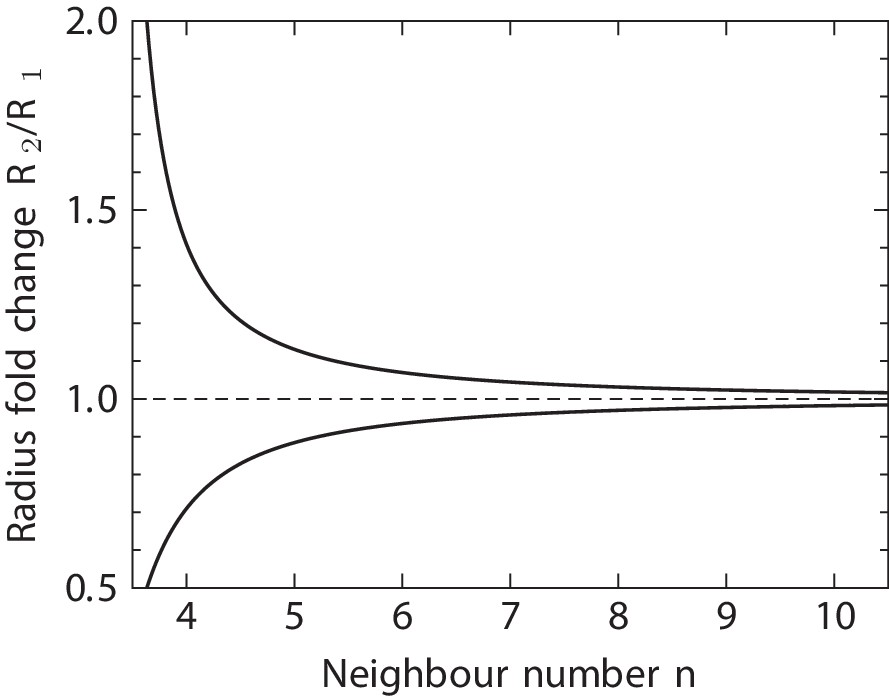
Predicted radius fold change in a tubular epithelium between a pair or consecutive T1 transitions per cell.
Additional files
Download links
A two-part list of links to download the article, or parts of the article, in various formats.
Downloads (link to download the article as PDF)
Open citations (links to open the citations from this article in various online reference manager services)
Cite this article (links to download the citations from this article in formats compatible with various reference manager tools)
3D cell neighbour dynamics in growing pseudostratified epithelia
eLife 10:e68135.
https://doi.org/10.7554/eLife.68135


