Unsupervised Bayesian Ising Approximation for decoding neural activity and other biological dictionaries
- Department of Medical Physics, Centro Atómico Bariloche and Instituto Balseiro, Argentina
- Department of Physics, Emory University, United States
- Department of Biology, Emory University, United States
- Initiative in Theory and Modeling of Living Systems, United States
Figures
Figure 1
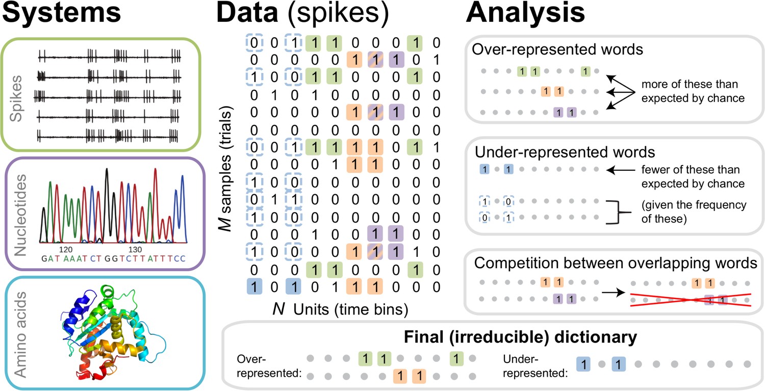
The dictionary reconstruction problem.
In many biological systems, such as understanding the neural code, identifying protein-DNA binding sites, or predicting 3-D protein structures, we need to infer dictionaries — the sets of statistically over- or under-represented features in the datasets (relative to some null model), which we refer to as words in the dictionary. To do so, we represent the data as a matrix of binary activities of biological units (spike/no spike, presence/absence of a mutation, etc.), and view different experimental instantiations as samples from an underlying stationary probability distribution. We then use the uBIA method to identify the significant words in the data. Specifically, uBIA systematically searches for combinatorial activity patterns that are over- or under-represented compared to their expectation given the marginal activity of the individual units. If multiple similar patterns can (partially) explain the same statistical regularities in the data, they compete with each other for importance, resulting in an irreducible dictionary of significant codewords. In different biological problems, such dictionaries can represent neural control words, DNA binding motifs, or conserved patterns of amino acids that must be neighbors in the 3-D protein structure.
Figure 2
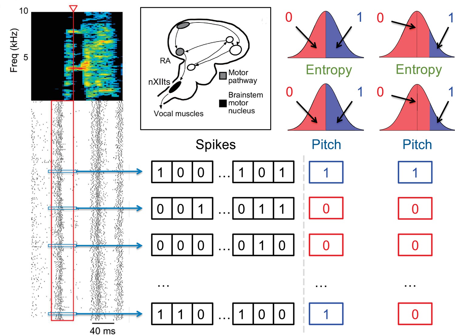
Quantification of the neural activity and the behavior.
A spectrogram of a single song syllable in top-left corner shows the acoustic power (color scale) at different frequencies as a function of time. Each tick mark (bottom-left) represents one spike and each row represents one instantiation of the syllable. We analyze spikes produced in a 40ms premotor window (red box) prior to the time when acoustic features were measured (red arrowhead). These spikes were binarized as 0 (no spike) or 1 (at least one spike) in 2ms bins, totaling 20 time bins. The different acoustic features (pitch, amplitude, spectral entropy) were also binarized. For different analyses in this paper, 0/1 can denote the behavioral feature that is below/above or above/below its median, or as not belonging/belonging to a specific percentile interval. The inset shows the area RA within the song pathway, two synapses away from the vocal muscles, from which these data were recorded.
Figure 3
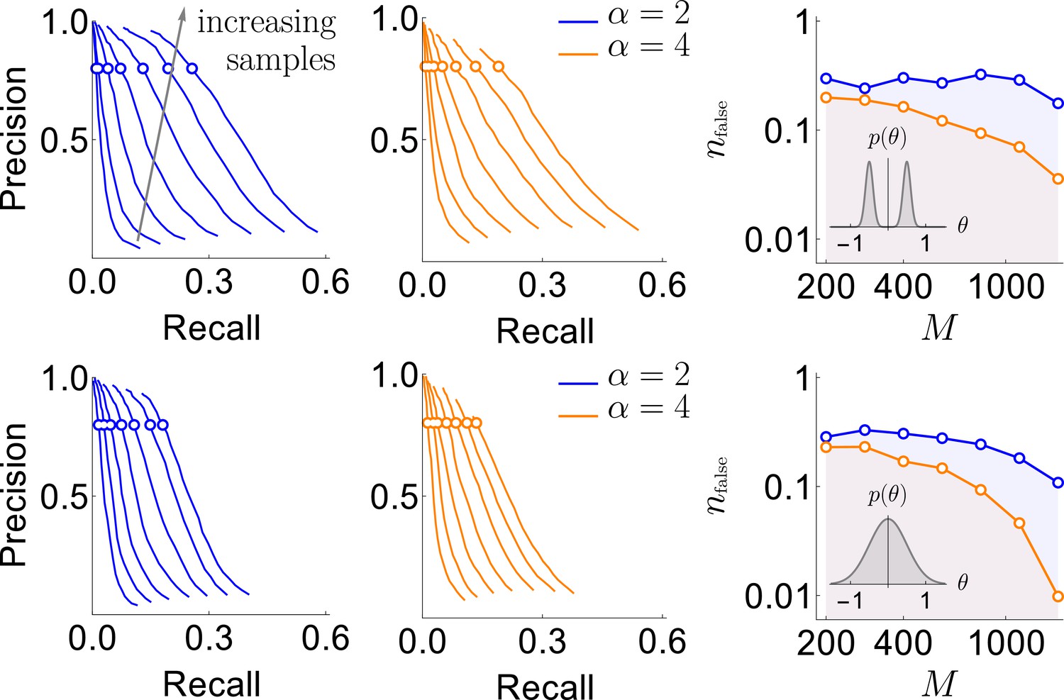
Results of the synthetic data analysis.
Performance on synthetic data as a function of the density of interactions α, the distributions for the strength of interactions, and the number of samples (logarithmically spaced). The first and the second columns correspond to precision-recall curves for the different density of interactions (significant words) per variable, , within the true generative model. The top and the bottom rows corresponds to the interaction strengths selected from the sum of two Gaussian distributions, or a single Gaussian, as described in the text. For the first two columns, we vary the significance threshold in marginal magnetization , such that the full false discovery rate on the shuffled data . In the third column we show the value of that corresponds to the precision of 80% as a function of (the number of samples), so that the precision is larger than in the shaded region. This region is quite large and overlaps considerably for the four cases analyzed, illustrating robustness of the method.
Figure 4
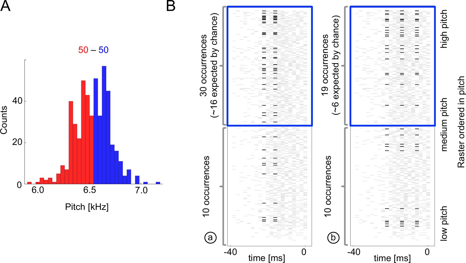
Sample multispike codewords.
(A) Probability distribution an acoustic parameter (fundamental frequency, or pitch). For this analysis, we consider the output to be when the pitch is above median (blue), and zero otherwise (red). (B) Distribution of two sample codewords (a two-spike word in the left raster, and a three-spike word in the right raster) conditional on pitch. In each raster plot, a row represents 40ms of the spiking activity preceding the syllable, with a grey tick denoting a spike. Every time a particular pattern is observed, its ticks are plotted in black. Note that these two spike words are codewords since they are overrepresented for above-median pitch (blue box) compared both to the null model based on the marginal expectation of individual spikes, and to the presence of the patterns in the low pitch region. Labels (a) and (b) identify these patterns in Figure 5B.
Figure 5
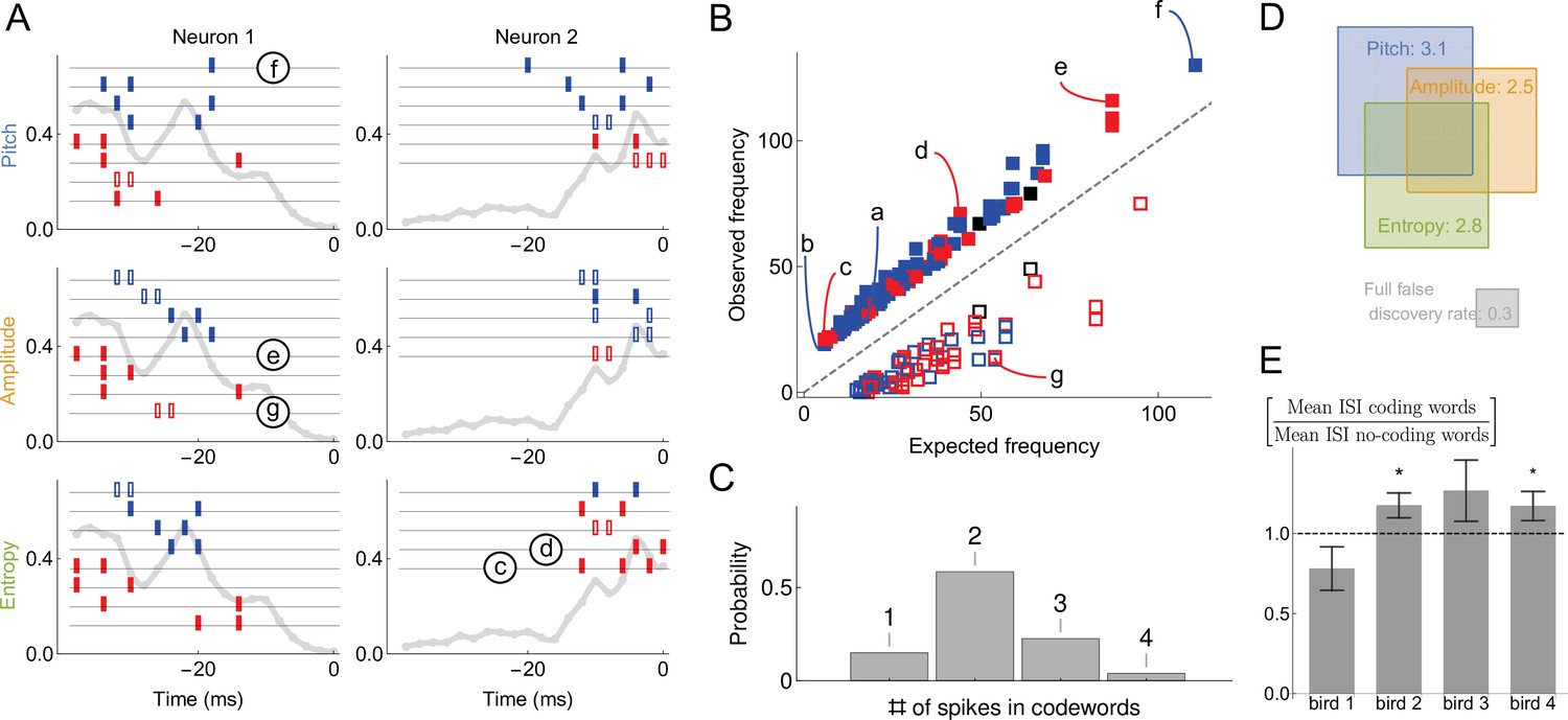
Statistical properties of neural dictionaries.
(A) Sample neural-behavioral dictionaries for two neurons from two different birds (columns) and for three different acoustic features of the song (rows: pitch, amplitude, and the spectral entropy). The light gray curve in the background and the vertical axis corresponds to the probability of neural firing in each 2ms bin (the firing rate). The rectangular tics represents the timing of spikes in neural words that predict the acoustic features. For example, a two spike word with tics at points corresponds to the probability that the word is a codeword for the acoustic feature with a probability statistically significantly higher than 1⁄2. Codewords for high (low) output, that is, above (below) the median, are shown in blue (red). Full (empty) symbols correspond to over(under)-occurrence of the codeword-behavior combinations compared to the null model. Finally full (empty) black symbols represent words that over(under)-occur in the blue code and under(over)-occur in the red code. Words labeled (c)-(g) are also shown in (B). (B) Frequency of occurrence of statistically significant codewords for different acoustic features in different neurons. Only first 200 codewords shown for clarity. Plotting conventions same as in (A), and letters label the same codewords as in (A) and in Figure 4B. (C) Proportion of -spike codewords found in the dictionaries analyzed. An -spike word corresponds to an -dimensional word in the neural-behavioral dictionary. Most of the significant codewords have two or more spikes in them. (D) Mean number of significant codewords, averaged across all neurons and acoustic features. An average neuron has 5.6 codewords in our dataset, of which 3.1 code for the pitch, 2.5 for the amplitude, and 2.8 for the spectral entropy, with the number of words coding for pairs of features or for all three of them indicated by the overlap of rectangles in the Venn diagram. For comparison, our estimated false discovery rate is 0.3 words, so that only ∼0.3 spurious words are expected to be discovered in each individual dictionary. We note that about a third of all analyzed dictionaries are empty, so that those that have words in them typically have more than illustrated here. (E) Mean inter-spike interval (ISI) for the codewords (spike words that code for behavior) vs. all spike words that are significantly over- or under-represented, but do not code for behavior. Averages in each of the four analyzed birds are shown, illustrating that the ISI statistics of the coding and non-coding words are different, but the differences themselves vary across the birds. Star denotes 95% confidence. Other properties of the dictionaries (mean number of spikes in codewords, fraction of codewords shared by three vocal features, proportion of under/over-occurring codewords), do not differ statistically significantly across the birds.
Figure 6
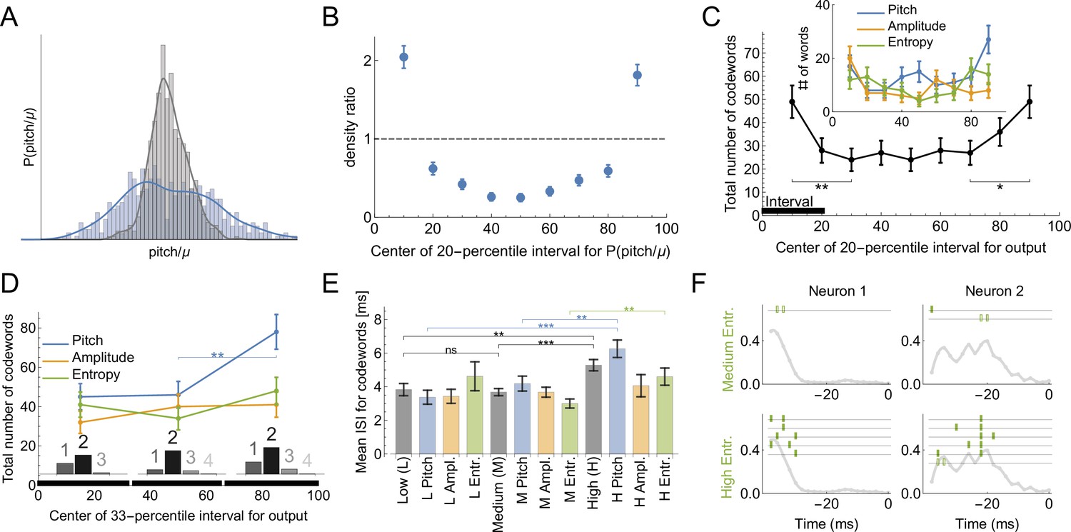
Codes for vocal motor exploration.
(A) Distribution of syllable pitch relative to the mean for exploratory and performance behaviors (blue, intact birds, vs. grey, LMAN-lesioned animals, see main text). (B) Ratio of the histograms in (A) evaluated in the quintiles of the exploratory (blue) distribution centered around [10%,20,...90%] points. (C) Total number of codewords when considering the vocal output as 1 if it belongs to a specific 20-percentile interval of the output distribution, and 0 otherwise. We observe that there are significantly more codewords for the exploratory behavior (tails of the distribution compared to the middle intervals). Notice that the shape of the curves parallels that in (B), suggesting that exploration drives the diversity of the codewords. (D) Number of codewords when considering the vocal output as 1 if it belongs to a 33-percentile (non-overlapping) interval of the output distribution, and 0 otherwise. Here there are significantly more codewords when coding for high pitch. Further, the codewords found for each of the three intervals are mostly multi-spike (histograms show the distribution of the order of the codewords for each percentile interval). (E) For codewords for the 33-percentile intervals, we compare the mean inter-spike intervals (ISIs). Codewords for high outputs (especially for pitch and spectral entropy) have a significantly larger mean ISI. (F) We illustrate dictionaries of two neurons for the medium and the high spectral entropy ranges. Notice that the high entropy range has significantly more codewords.
Figure 7
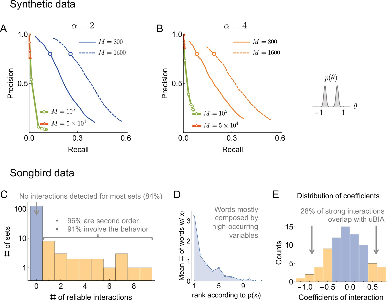
Comparison of Ganmor et al.method to uBIA.
(A, B) For the synthetic data that we consider in the paper (Figure 3, interactions arising from the sum of two Gaussians), we obtained precision vs recall curves for the Ganmor et al. method (green and red) using a sweep over the absolute value of the inferred interaction threshold and comparing the detected interactions to the true ones. We also show the corresponding uBIA curves (blue) from Figure 3 for . As illustrated, the Ganmor approach requires two orders of magnitude more data to begin discovering interactions and still does not reach the performance of uBIA for datasets with realistic sizes. (C) For the songbird data, the Ganmor et al. approach did not detect any interactions for most datasets. Of the 82 interactions that were detected, most corresponded to pairwise interaction between the behavior and the time bin. (D) Words identified by the Ganmor et al. were largely detected based on high marginal probability, consistent with an inability to detect higher order patterns directly. (E) The most significant detected interactions (largest interaction coefficients) generally overlap with words detected by uBIA.
Figure 8
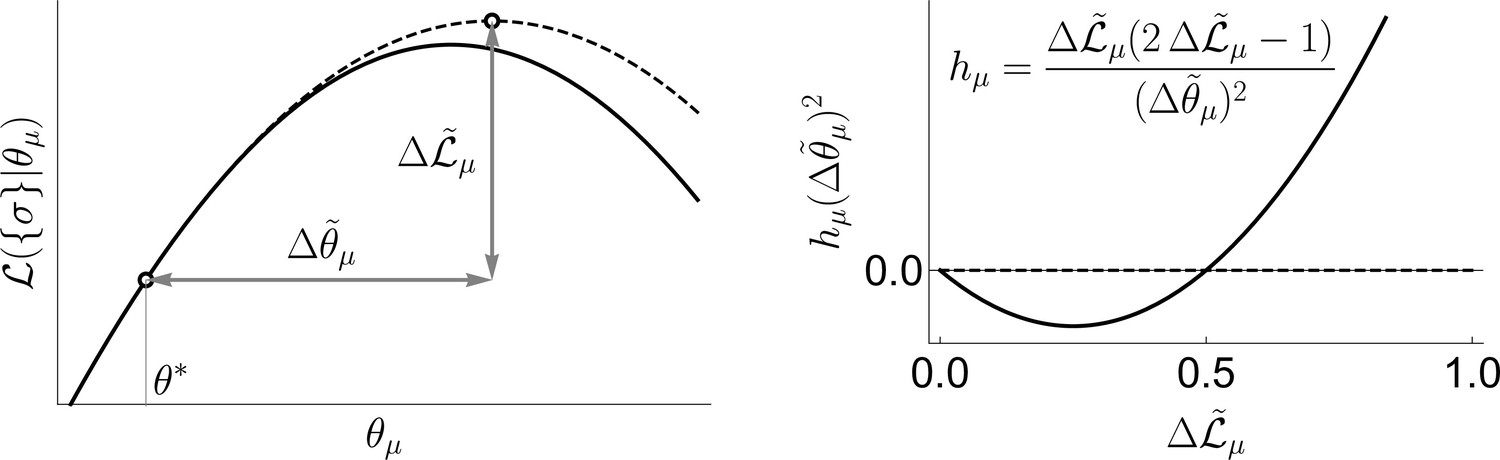
Geometric interpretation of the fields in the uBIA method, in relation to the log-likelihood function .
The uBIA method makes an approximate guess (dashed line in left panel) of how much in log-likelihood we would win be fitting a parameter , and how far in parameter space we would need to go, (see left panel). The sign of the field only depends on the improvement in log-likelihood, being positive beyond a threshold (inclusion of a word). This complexity penalty comes from the Bayesian approach in this strong regularized regime. On the other hand, the farther we go in parameter space, the smaller in absolute value the field becomes (see right panel).
Figure 9
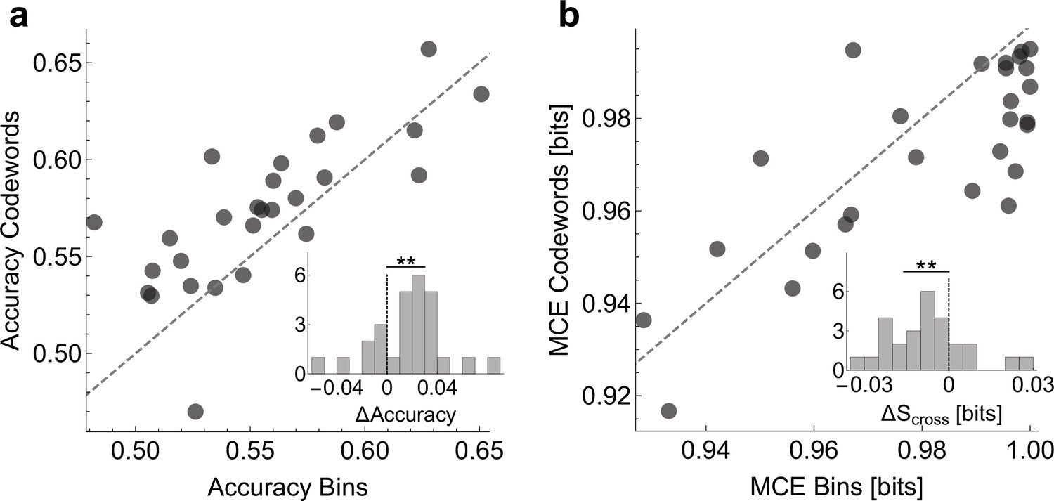
Prediction accuracy with uBIA dictionaries.
We compare prediction of the behavior using logistic regression models that have as features (i) neural activity in all the time bins at 2ms resolution versus (ii) only the detected relevant codewords. (A) Scatter plot of accuracy of models of both types, evaluated using twofold cross-validation. Inset shows that the different between the prediction is significant with according to the paired t-test. (B) Scatter plots of the mean cross-entropy between the data and the models for the two model classes. Inset: Even though the models that use the codewords are simpler (have fewer terms), they are able to predict better (with lower cross-entropy) according to the paired t-test.
Additional files
Download links
A two-part list of links to download the article, or parts of the article, in various formats.
Downloads (link to download the article as PDF)
Open citations (links to open the citations from this article in various online reference manager services)
Cite this article (links to download the citations from this article in formats compatible with various reference manager tools)
Unsupervised Bayesian Ising Approximation for decoding neural activity and other biological dictionaries
eLife 11:e68192.
https://doi.org/10.7554/eLife.68192


