Figures and data in Learning developmental mode dynamics from single-cell trajectories | eLife

Figures
Videos
Additional files

12 figures, 4 videos and 1 additional file

Figures

Figure 1 with 1 supplement

Download asset Open asset

From single-cell tracking data to sparse mode amplitude representations.

(A) Microscopic imaging data of early zebrafish development (adapted from Figure 1b in Kobitski et al., 2015) shows cell migration from an initially homogeneous pole of cells (left) toward an elongated structure that indicates the head-tail axis of the fully developed organism. Scale bar, $100 μ m$ . (B) Experimental single-cell tracking data from Shah et al., 2019 (blue dots) during similar developmental time points (±20 min) as in A. $t = 0$ min for the indicated time points in B corresponds to a developmental time of 4 hours post fertilization. The $z$ -axis points from the ventral pole (VP) to the animal pole (AP). (C) Coarse-grained relative cell density $ρ (r, t)$ (color) and associated coarse-grained flux $J (r, t)$ (streamlines) determined from single cell positions and velocities from data in B via Equation 2a. Thickness of streamlines is proportional to the logarithm of the spatial average of $| J |$ (see Video 1). (D) Dynamic harmonic mode representation of the relative density $ρ (r, t)$ (Equation 4, left panel) and of the flux $J (r, t)$ (Equation 5, middle and right panel) for fields shown in C. The modes $j_{l m}^{(1)}$ correspond to compressible, divergent cell motion, the modes $j_{l m}^{(2)}$ describe incompressible, rotational cell motion. Mode amplitudes become negligible for $l \geq 5$ (Video 2). For all panels, horizontal black lines delineate blocks of constant harmonic mode number $l$ and black triangles denote the end of epiboly phase.

Figure 1—figure supplement 1

Download asset Open asset

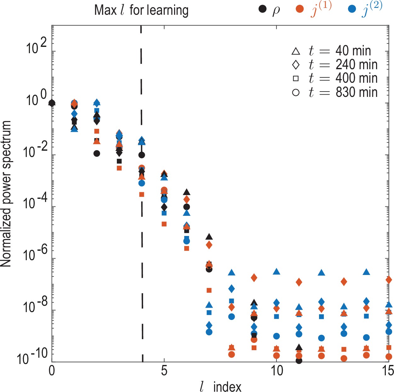
Convergence of spectral representation.

Decay of power spectra for coarse-grained experimental density and flux fields. Rotationally invariant spatial power spectra as a function of the mode $l$ index were computed for the density field $ρ$ as $P_{ρ, l} = \sum_{m = - l}^{l} ρ_{l m}^{2}$ and for modes contributing to cell fluxes ( $j^{(1)}$ and $j^{(2)}$ ) as $P_{j k, l} = \sum_{m = - l}^{l} [j_{l m}^{(k)}]^{2}$ for $k = 1, 2$ . Spectra were computed at representative timepoints $t = 40, 240, 400, 830$ min and normalized by their maximum value. The observed decay indicates that a spectral representations of the coarse-grained fields is meaningful, and shows that the mode cut-off chosen for the learning ( $l \leq 4$ ) amounts to discarding approximately 1% of spectral power in each field.

Figure 2 with 4 supplements

Download asset Open asset

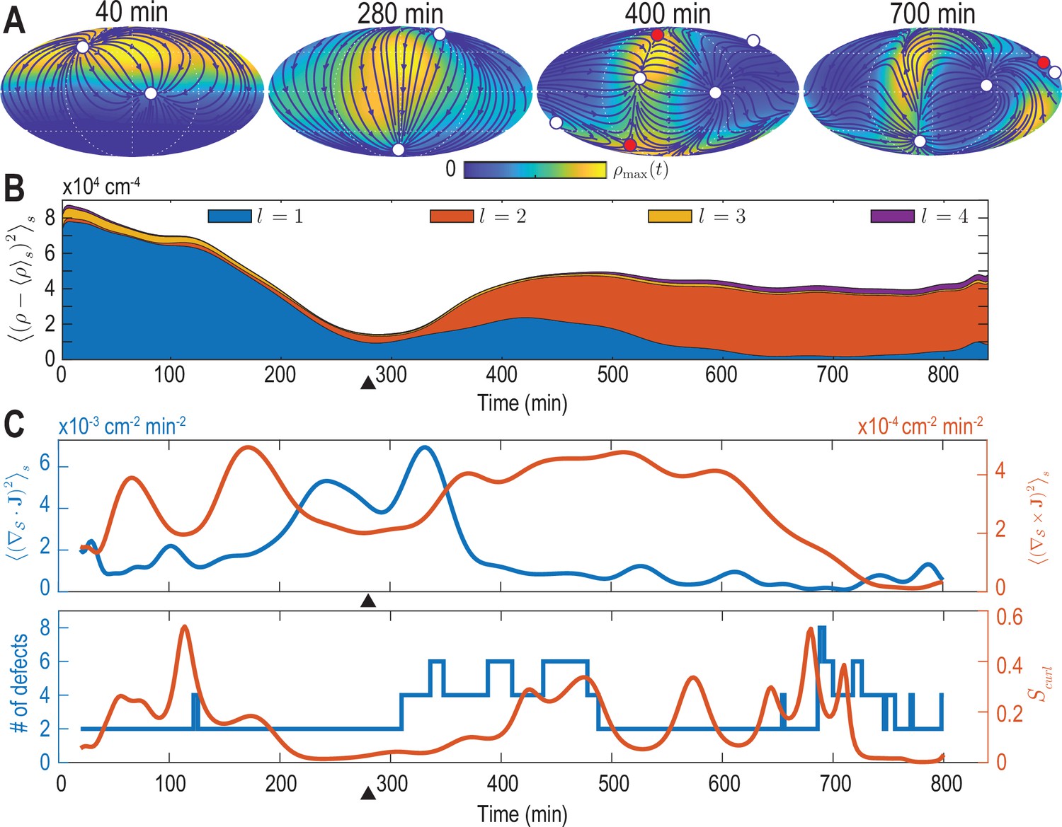
Mode signatures of developmental symmetry breaking and topological defects in cellular flux.

(A) Two-dimensional Mollweide projection of the compressed coarse-grained density field $ρ (r, t)$ (colormap) and of the coarse-grained cell flux $J (r, t)$ (streamlines) at different time points of zebrafish gastrulation.White circles depict topological defects of charge +1 in the flux vector field, red circles depict defects with charge -1. The total defect charge is 2 at all times. Defects are seen to ‘lead’ the large-scale motion of cells and later localize mostly along the curve defined by the forming spine. Animal pole (AP) and ventral pole (VP) are located at top and bottom, respectively. (B) Density fluctuations as a function of developmental time (see Equation 9), broken down in contributions from different harmonic modes $l$ . The underlying symmetry breaking is highlighted prominently by this representation: During the first 75% of epiboly (0–280 min) cells migrate away from, but are still mostly located near the animal pole, presenting a density pattern with polar symmetry ( $l = 1$ ). During the following convergent extension phase cells converge towards a confined elongated region that is ‘wrapped’ around the yolk, corresponding to a density pattern with nematic symmetry ( $l = 2$ ). Black triangles indicate transition from epiboly to convergent extension. (C) Comparison of surface averaged divergence $\nabla_{S} \cdot J$ and curl $\nabla_{S} \times J$ of the cellular flux computed via Equation 10a and Equation 10b, respectively (top). A relative curl amplitude $S_{c u r l}$ computed from these quantities via Equation 11 correlates with the appearance of an increased number of topological defects in the cell flux (bottom), suggesting that incompressible, rotational cell flux is associated with the formation of defects.

Figure 2—figure supplement 1

Download asset Open asset

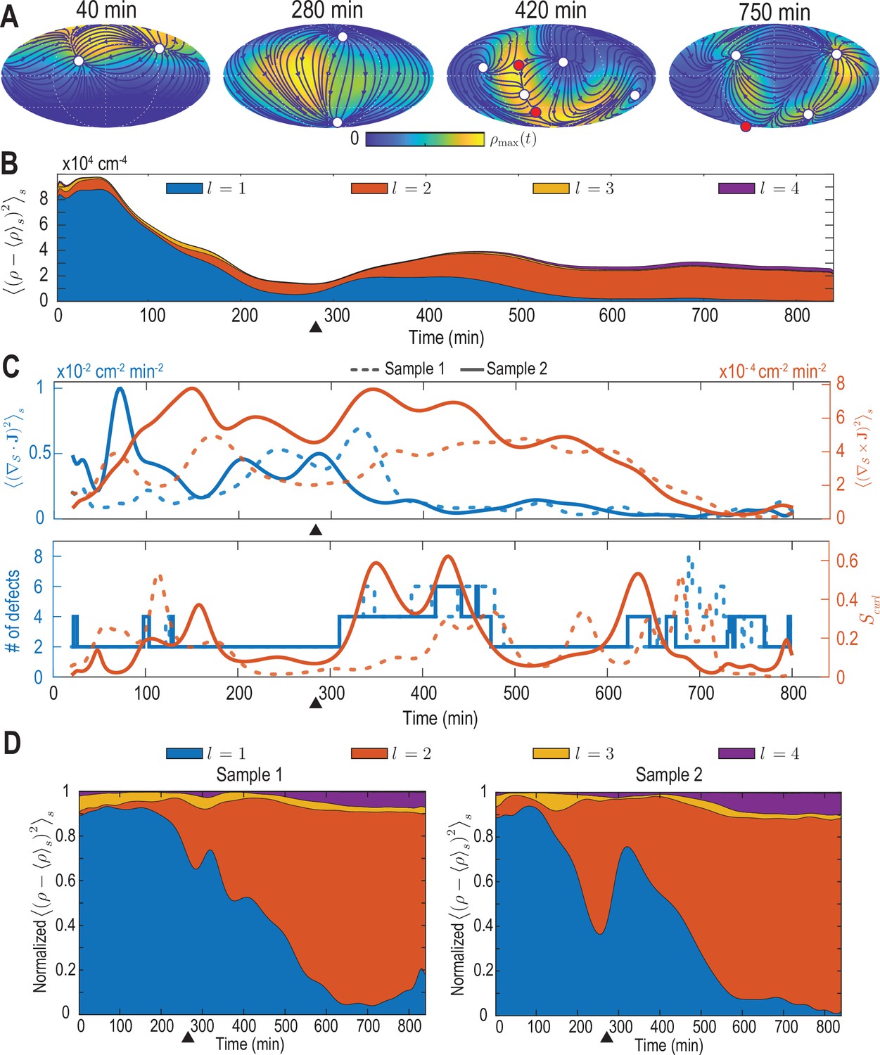
Analysis of the harmonic mode representation for a second experimental dataset.

(A–C) Analysis presented in Figure 2A–C of the main text performed on a second cell-tracking dataset (‘Sample 2’). In C, solid lines indicate results for Sample 2, dashed lines correspond to the results for the dataset discussed in the main text (‘Sample 1’). (D) Contributions to density fluctuations from both samples, broken down into contributions from different modes with harmonic mode number $l$ and normalized at each time point by the total fluctuation intensity. Black triangles indicate the completion of epiboly.

Figure 2—figure supplement 2

Download asset Open asset

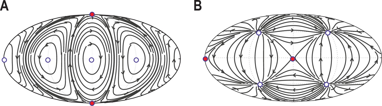
Validation of automated defect tracking.

Demonstration of the defect tracking on two example tangential vector fields on a spherical surface. (A) Vector field defined by $J = Φ_{(2, 2)}$ . (B) Vector field defined by $J = Ψ_{(2, - 1)} + 0.1 Φ_{(2, 2)}$ . Black lines depict the streamlines defined by these vector fields. White circles depict topological defects of charge +1, red circles depict defects with charge -1. For further details of the tracking approach see Materials and Methods.

Figure 2—figure supplement 3

Download asset Open asset

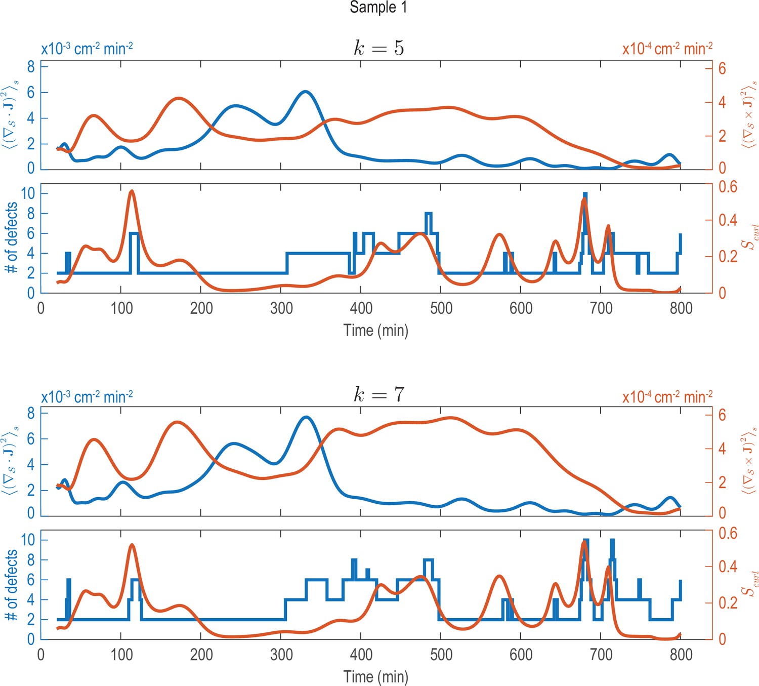
Analysis of fluxes and defects for different coarse-graining length scales (Sample 1).

Analysis shown in Figure 2C performed on data that was coarse-grained with different coarse-graining length scales, represented by the parameter $k$ (see Appendix 1—figure 2). Choosing larger ( $k = 5$ ) or smaller ( $k = 7$ ) coarse-graining length scales than used in Figure 2C ( $k = 6$ ), key signatures extracted from the data (dominant phases of divergent and rotary flows and a correlation between increased defect dynamics and cellular fluxes with curl) can still be robustly recovered.

Figure 2—figure supplement 4

Download asset Open asset

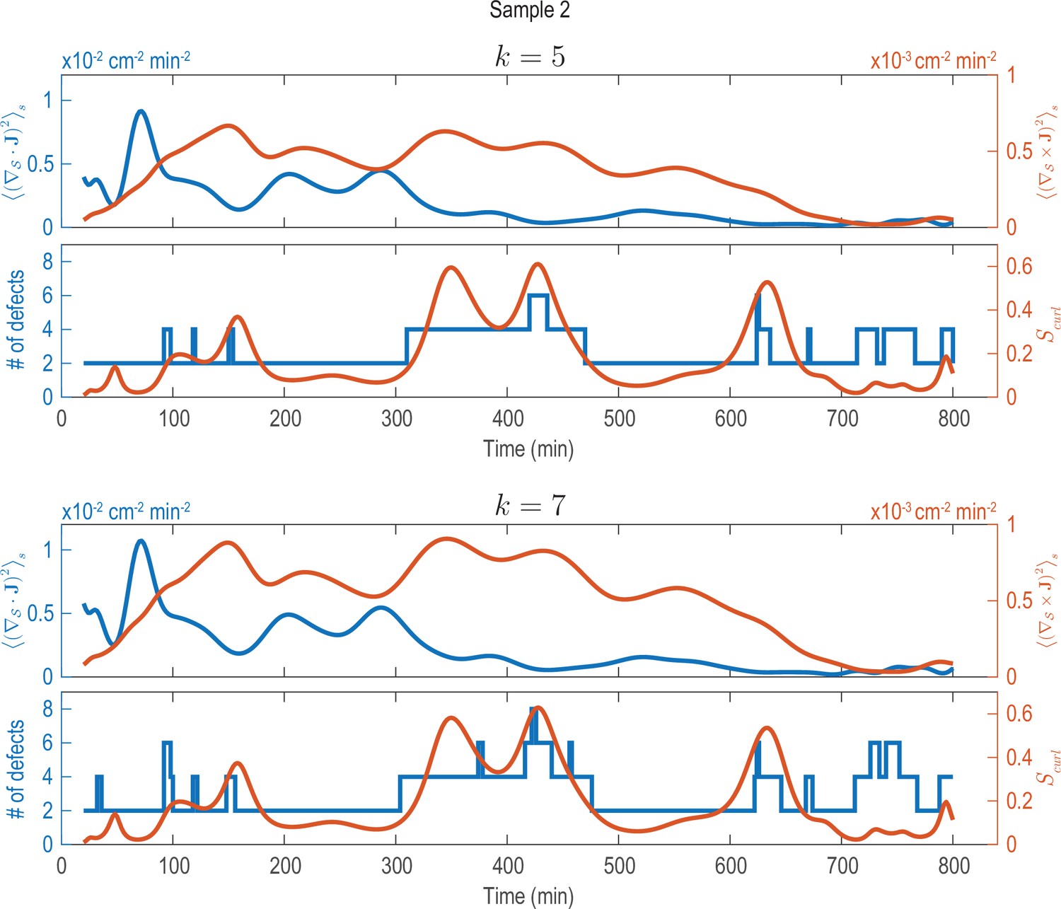
Analysis of fluxes and defects for different coarse-graining length scales (Sample 2).

Analysis shown in Figure 2—figure supplement 1C (solid lines) performed on data that was coarse-grained with different coarse-graining length scales, represented by the parameter $k$ (see Appendix 1—figure 2). Choosing larger ( $k = 5$ ) or smaller ( $k = 7$ ) coarse-graining length scales than used in Figure 2—figure supplement 1C ( $k = 6$ ), key signatures extracted from the data (dominant phases of divergent and rotary flows and a correlation between increased defect dynamics and cellular fluxes with curl) can still be robustly recovered.

Figure 3

Download asset Open asset

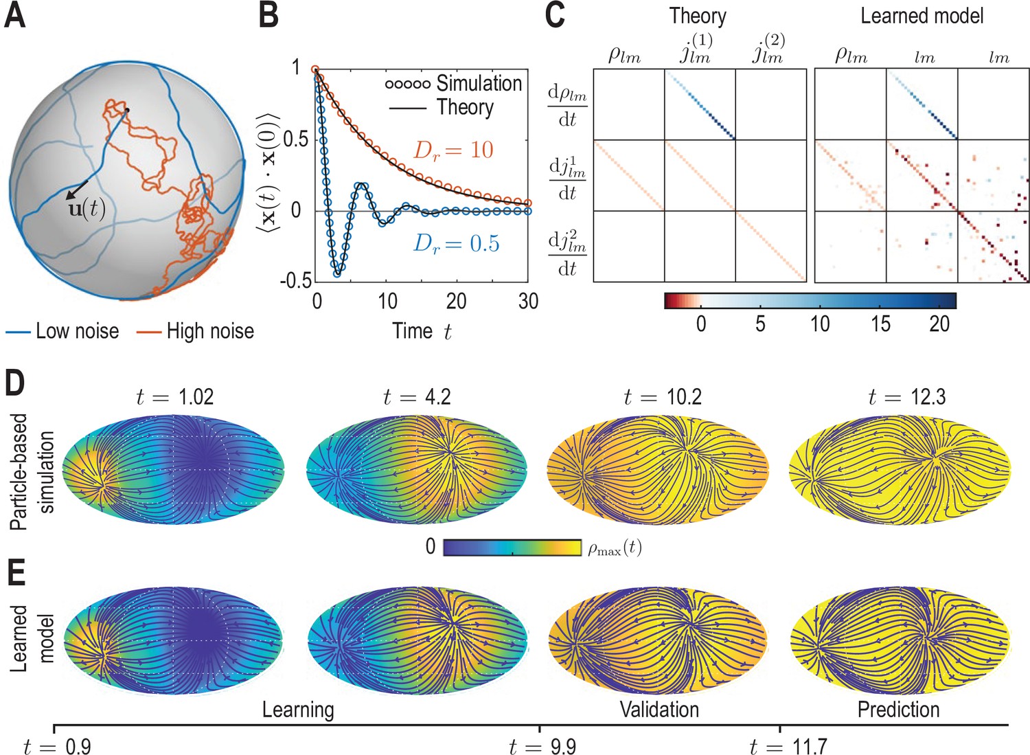
Learning active Brownian particle (ABP) dynamics on a sphere.

(A) ABPs move on a unit sphere (radius $R_{0} = 1$ ) with angular speed $v_{0} = 1$ along a tangential unit vector $u (t)$ that is subject to stochastic in-plane fluctuations (see Appendix 3 for further details). Example single-particle trajectories are shown in the high-noise (orange, $D_{r} = 10$ in units of $R_{0} v_{0}$ ) and in the low-noise regime (blue, $D_{r} = 0.5$ ). Time $t$ is measured in units of $R_{0} / v_{0}$ in all panels. (B) Position correlation function $⟨ x (t) \cdot x (0) ⟩$ averaged over $3 \times 10^{4}$ independent ABP trajectories show distinct oscillations of period $\approx 2 π$ in the low-noise regime, as ABPs orbit the spherical surface more persistently (see Video 3). Standard error of the mean is smaller than symbol size. (C) Analytically predicted (left) and inferred (right) dynamical matrices $M$ (see Equation 12) describing the mean-field dynamics of a large collection of non-interacting ABPs (see Equation 13a, Equation 13b, Equation 13c and Appendix 3) show good quantitative agreement. (D) Mollweide projections of coarse-grained ABP simulations with $v_{0} = 1$ and $D_{r} = 0.5$ using cell positions from the first time point in the zebrafish data (Figure 1) as the initial condition: At each position 60 particles with random orientation were generated and their ABP dynamics simulated, amounting to approximately $1.2 \times 10^{5}$ particles in total. The density fields homogenize over time, where the maximum density at $t = 12.3$ has decayed to about 5% of the maximum density at $t = 1.02$ . Blue lines and arrows indicate streamlines of the cell flux $J (r, t)$ . (E) Simulation of the learned linear model, Equation 12 with $M$ shown in (C) (right), for the same initial condition as in D. Marked time points indicate intervals of learning, validation and prediction phases of the model inference (see Appendix 4).

Figure 4 with 1 supplement

Download asset Open asset

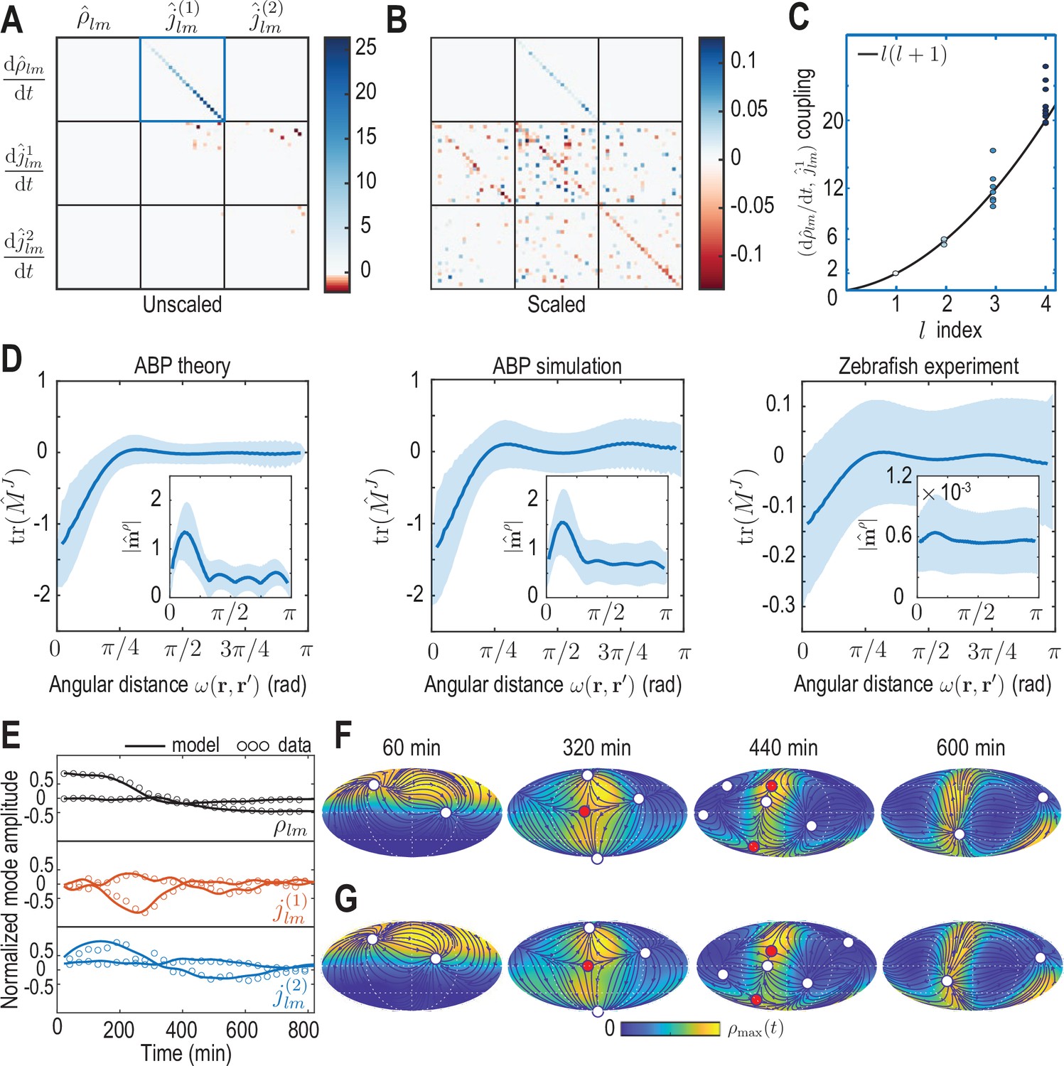
Model learning for experimental data of collective cell motion during early zebrafish development.

(A) Visualization of the constant mode coupling matrix $M$ that was learned from experimental data (see Appendix 4) and describes the dynamics of the mode vector $a = {[ρ_{l m} (t), j_{l m}^{(1)} (t), j_{l m}^{(2)} (t)]}^{T}$ via Equation 12. Dimensionless fields are defined by ${\hat{ρ}}_{l m} = R_{s}^{2} ρ_{l m}$ and ${\hat{j}}_{l m}^{(i)} = R_{s} Δ t j_{l m}^{(i)}$ ( $i = 1, 2$ ) with $R_{s} = 300 μ m$ and $Δ t = 2$ min. (B) Scaling the learned matrix $M$ by the Mean Absolute Deviation (MAD) of the modes (see Appendix 4) reveals structures reminiscent of the mode coupling matrix learned for ABPs (Figure 3C). (C) The learned model recovers mass conservation in mode space (Equation 6). (D) Comparison of theoretical and inferred real-space kernels (see Equation 14 and Appendix 4) for the ABP dynamics and for the experimental data of collective cell motion. The trace of the non-dimensional kernel ${\hat{M}}^{J} (r, r^{'})$ (the only non-zero eigenvalue, Appendix 4—figure 2) indicates a localized flux-flux coupling with a similar profile among both systems. The oscillating magnitude of the non-dimensionalized density-flux kernel $| {\hat{m}}^{ρ} (r, r^{'}) |$ (insets) in the ABP system indicates a gradient-like coupling and is consequence of the persistent ABP motion. In the experimental data, a first peak around $ω = π / 4$ is also visible, but less pronounced. All kernel properties were computed by averaging over pairs of positions $r, r^{'}$ that are separated by the same angular distance $ω = \arccos (r \cdot r^{'}) \in [0, π]$ . Solid lines indicate mean, shaded areas indicate standard deviation. (E) Comparison of experimental mode dynamics (circles) with numerical solution (solid line) of the minimal model Equation 12 for learned matrix $M$ visualized in A. For clarity, the comparison is shown for the two dominant modes of each set of harmonic modes $ρ_{l m}, j_{l m}^{(1)}$ and $j_{l m}^{(2)}$ . (F, G) Mollweide projections of the experimental data (F) and of the numerical solution of the learned model (G) show very good agreement (Video 4). Blue lines and arrows illustrate streamlines defined by the cell flux $J (r, t)$ , circles depict defects with topological charge +1 (white) and -1 (red).

Figure 4—figure supplement 1

Download asset Open asset

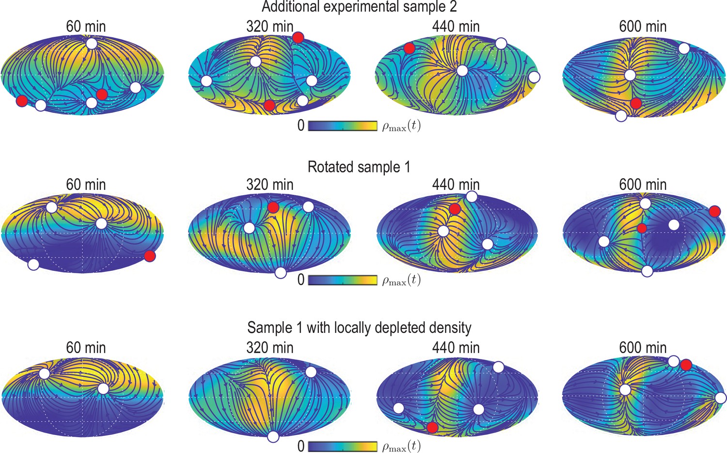
Simulating the learned model with different initial conditions.

Mollweide projections from simulations of the model Equation 12 with $M$ depicted in Figure 4B that was learned for experimental data from sample 1, but using different initial conditions (from top to bottom): initial condition from experimental data set sample 2 (Figure 2—figure supplement 1); initial condition from sample 1 rotated by 10° away from the animal pole; initial condition from sample one with $ϵ = 10$ % of the density at the animal pole removed. For the latter, the initial density field of sample one is multiplied by a factor $1 - ϵ f_{6} (θ)$ , where $f_{6} (θ)$ denotes the $k = 6$ density coarse-graining kernel (see Appendix 1) evaluated at polar angle $θ$ . Blue lines and arrows illustrate streamlines defined by the cell flux $J (r, t)$ , circles depict defects with topological charge +1 (white) and -1 (red).

Appendix 1—figure 1

Download asset Open asset

Illustration of the action of the coarse-graining tensor kernel $K {(r, r^{'})}_{i j^{'}}$ Equation 19.

Left: $K_{i j^{'}}$ acts in the two tangent space at points $r$ and $r^{'}$ that are separated by an angular distance $ω = acos (r \cdot r^{'})$ . Each tangent plane has corresponding basis vectors, $e_{i}$ $e_{i^{'}}$ for $i = 1, 2$ . Right: The tensor kernel $K_{i j^{'}} \sim e_{i} \cdot e_{j^{'}}$ projects vectors $u$ in the tangent space of $r^{'}$ and generates a vector $v$ tangent at $r$ .

Appendix 1—figure 2

Download asset Open asset

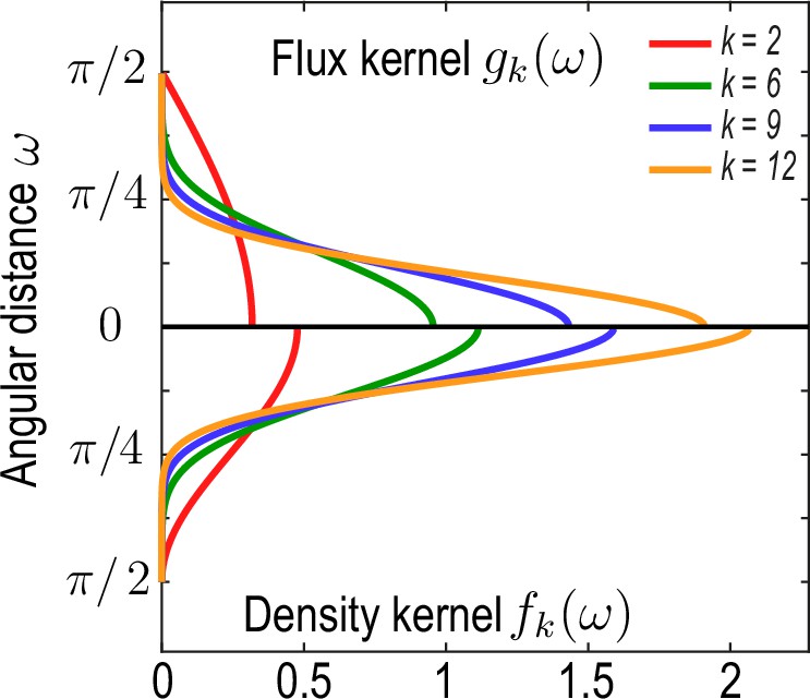
Family of kernel functions $f_{k} (ω)$ and $g_{k} (ω)$ given in Equation 26a.

These functions represent weights of the coarse-graining kernels Equation 22a and Equation 22b that are defined such that the kernels satisfy the consistency relation Equation 19. $ω = acos (r \cdot r^{'})$ denotes angular distances between $r$ and. $r^{'}$ Coarse-graining of a conserved number of particles on a sphere to determine a density field $ρ$ (Equation 2a, main text) requires a different weighting – $f_{k} (ω)$ – than the coarse-graining of an associated flux $J$ (Equation 2b , main text), which requires a weighting $g_{k} (ω)$ instead to ensure that coarse-grained fields obey mass conservation Equation 18. A characteristic coarse-graining length scale associated with these kernels is the half-width at half-maximum (HWHM), which is related to $k$ by HWHM $= \arccos (2^{- 1 / k})$ .

Appendix 2—figure 1

Download asset Open asset

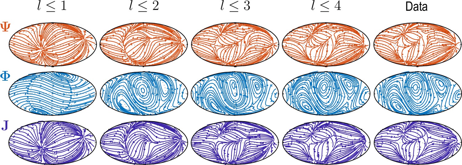
Sequentially adding vector spherical harmonics $Ψ_{l m}$ and $Φ_{l m}$ – equivalent to increasing $l_{max}$ in Equation 5 – resolves increasing levels of details present in experimental flux fields ("Data").

Main features of the data are captured already by a relatively small number of modes ( $l_{max} = 4$ used throughout this work).

Appendix 2—figure 2

Download asset Open asset

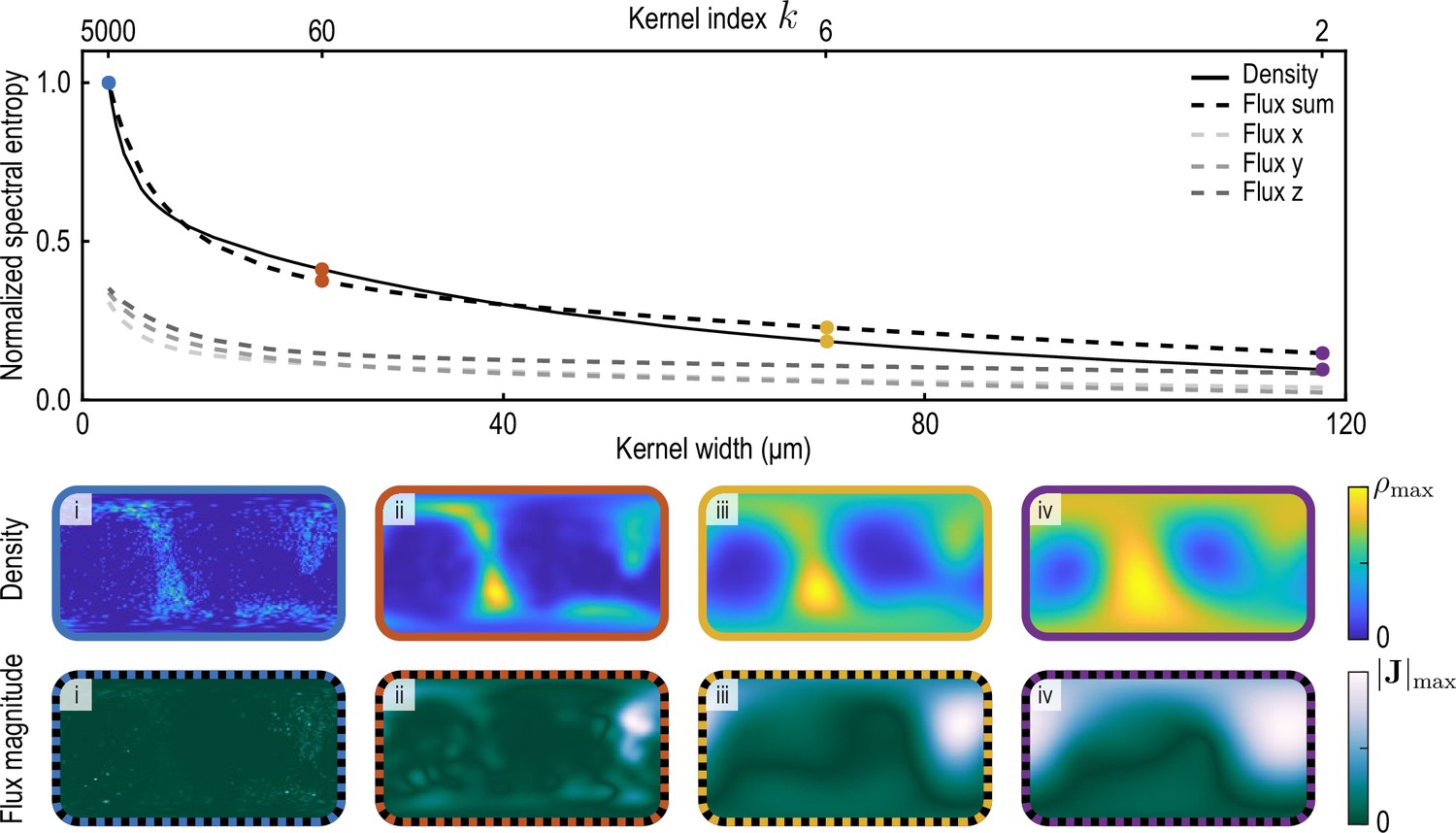
Normalized spectral entropy as a function of the coarse-graining kernel width (top) computed for density $ρ$ and flux field $J$ using Equation 34.

To evaluate the spectral entropy for the vector-valued flux, we define $S (J) := S (J_{x}) + S (J_{y}) + S (J_{z})$ (‘Flux sum’). The coarse-graining width – the half-width at half-maximum (HWHM) of the coarse-graining kernels Equation 22a and Equation 22b with weight functions Equation 26a – is varied by varying the kernel index $k$ , where $HWHM = \arccos (2^{- 1 / k})$ (see Appendix 1—figure 2). The fields $ρ$ and $| J |$ are shown in the two bottom rows for different values of $k$ i. $k = 5000$ (blue, data used to compute the reference spectral entropies $S_{0} (ρ)$ and $S_{0} (J)$ ) ii. $k = 60$ (brown) iii. $k = 6$ (yellow, used in main text) iv. $k = 2$ (purple).

Appendix 2—figure 3

Download asset Open asset

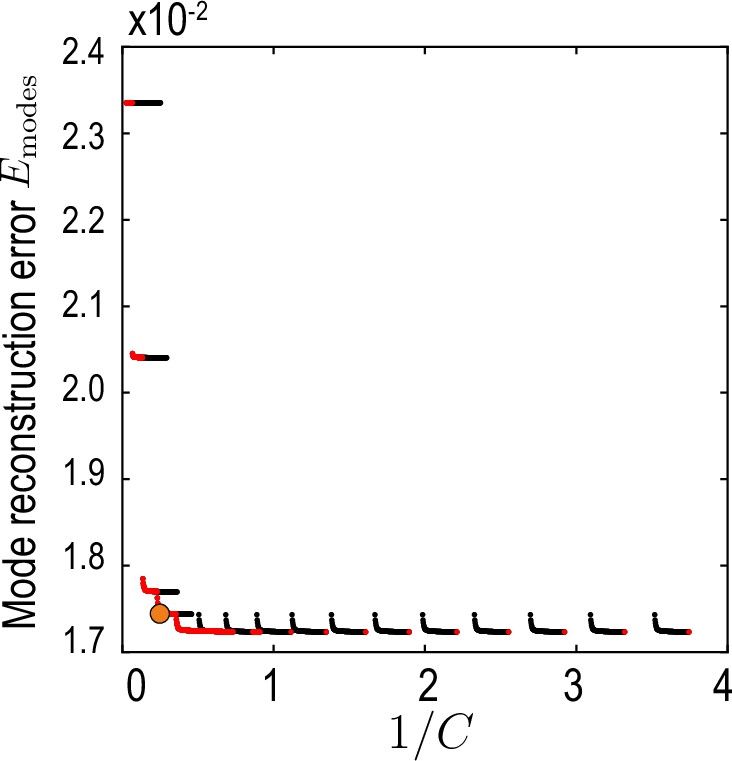
Relative average mode reconstruction error $E_{modes} (n_{max}, l_{max})$ Equation 36.

As a function of the inverse of the compression $C$ defined in Equation 35. Red points indicate the Pareto front (Jin and Sendhoff, 2008) of this compression-accuracy approximation trade-off. Orange circle indicates the final value used for our analysis.

Appendix 2—figure 4

Download asset Open asset

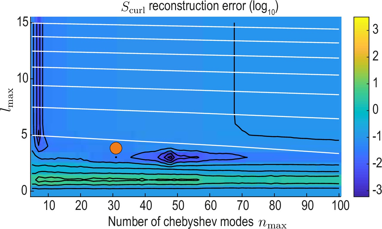
$S_{curl}$ reconstruction error landscape (log scale) as a function of $l_{max}$ and $n_{max}$ .

Black contour lines indicate iso-error lines (see Equation 37, $E_{curl} =$ const.), whereas white contour lines indicate iso-compression levels (see Equation 35, $C =$ const.). Orange circle indicates the final value used for our analysis.

Appendix 4—figure 1

Download asset Open asset

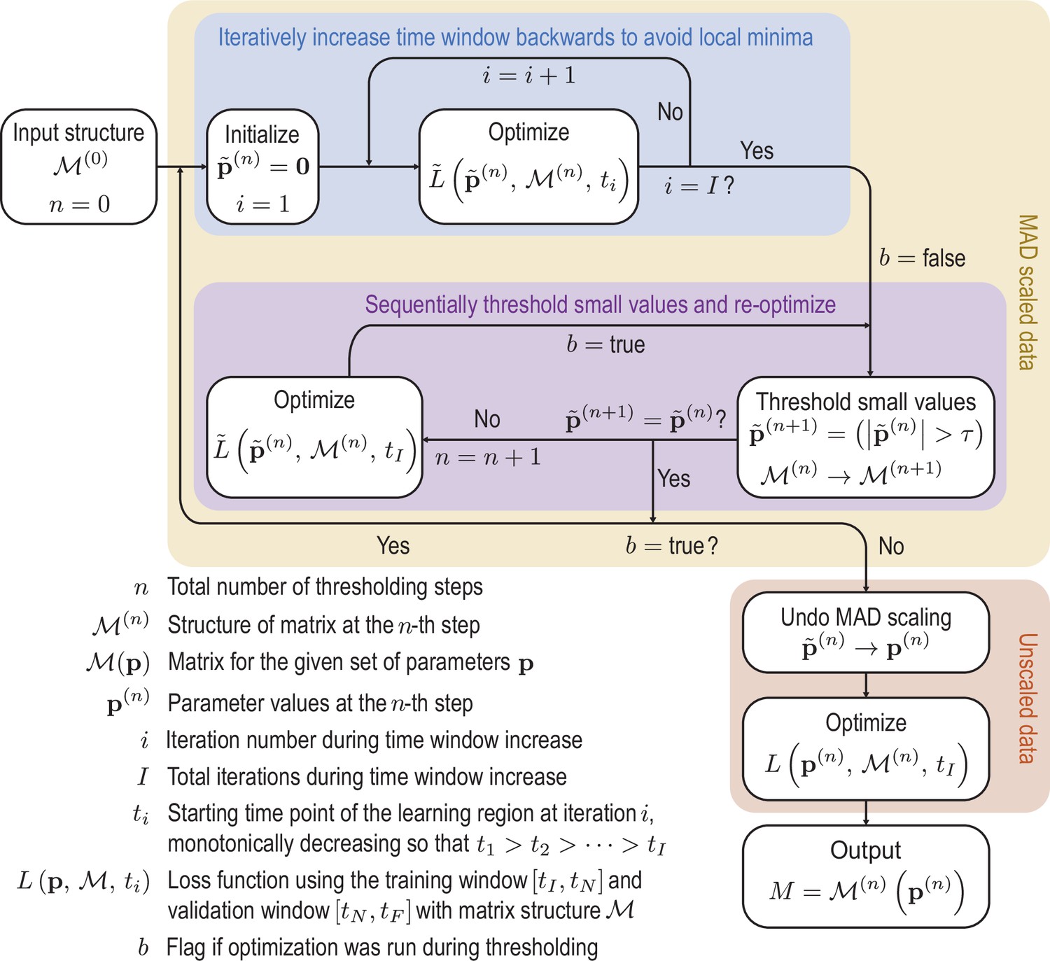
Initially the data is rescaled using the median absolute deviation (MAD) defined in Equation 50 to account for variation in scales across the modes.

Scaled variables are denoted by tildes. To avoid local minima of the optimization function, we iteratively feed more data into the cost function. Next we sequentially threshold the small terms in the matrix until convergence is reached. These procedures are repeated until the sparsity pattern converges. Finally the scaling is undone and the parameters are optimized on the unscaled data to produce the final matrix. Schematic of the learning procedure.

Appendix 4—figure 2

Download asset Open asset

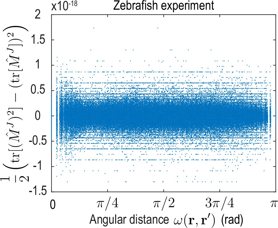
The $3 \times 3$ -matrix invariant $I_{2} = \frac{1}{2} (tr [{(M^{J})}^{2}] - {(tr [M^{J}])}^{2})$ sampled for pairs of positions $r$ , $r^{'}$ vanishes to machine precision for the dynamical matrix $M$ learned on the zebrafish data.

This invariant can be expressed in terms of matrix eigenvalues as $I_{2} = λ_{1} λ_{2} + λ_{1} λ_{3} + λ_{2} λ_{3}$ . Additionally, $λ_{1} λ_{2} λ_{3} = \det (M^{J}) = 0$ (see discussion below Equation 53), which implies only one eigenvalue is non-zero. Evaluating I₂ for the kernel matrix $M^{J}$ encoded by the theoretical (see Equation 13b and Equation 13c) and inferred (see Figure 3C, main text) dynamical matrix $M$ of the ABP dynamics yields similar results.

Videos

Video 1

Download asset

posterframe for video — Time evolution of the pre-processed cell tracking data (point cloud, see Materials and methods), and of the density field $ρ (r, t)$ (colormap) and associated flux $J (r, t)$ (streamlines) corresponding to the harmonic modes ${ρ_{l m}, j_{l m}^{(1)}, j_{l m}^{(2)}}$ shown in Figure 1D.

This mode representation was determined by the coarse-graining and projection procedure described in the main text. Streamline thickness is proportional to the logarithm of the average flux amplitude ${⟨ | J | ⟩}_{s}$ . For visualization purposes, cell distances to the origin were rescaled by a factor of $1.2 R_{s} / ⟨ R (t) ⟩$ , where $⟨ R (t) ⟩$ is the average cell distance from center at time $t$ and $R_{s} = 300 μ m$ is the mid-surface radius.

Video 2

Download asset

posterframe for video — Reconstruction of the hydrodynamics fields in real space by adding consecutive scalar and vector spherical harmonic modes of progressively higher order $l$ .

Surface coloring depicts the density field $ρ (r, t)$ , the associated flux $J (r, t)$ is indicated by streamlines. Streamline thickness is proportional to the logarithm of the average flux amplitude ${⟨ | J | ⟩}_{s}$ . The shown fields correspond to the time point $t = 420$ min in Video 1.

Video 3

Download asset

posterframe for video — Coarse-grained dynamics of active Brownian particles on the unit sphere in the low-noise ( $D_{r} = 0.5$ ) and high-noise ( $D_{r} = 10$ ) regime.

Data from $N = 3 \times 10^{4}$ independent ABP simulations was coarse-grained using the kernels $f_{k} (ω)$ and $g_{k} (ω)$ ( $k = 6$ ) described in Appendix 1. Initial ABP positions were sampled from an axisymmetric distribution with $p (θ) \propto \cos θ 1_{{θ §lt; π / 2}}$ . Mollweide projections in the left and right column are color-coded for density and flux magnitude $| J (r, t) |$ , respectively. Colormaps are normalized by the maximum values of density and flux magnitude fields across all time points.

Video 4

Download asset

posterframe for video — Comparison of dynamics of the experimental and learned density $ρ (r, t)$ (colormap) and flux fields $J (r, t)$ (streamlines) represented in a Mollweide projection.

White circles depict topological defects of charge +1 in the vector field $J (r, t)$ , red circles depict defects with charge -1. The total defect charge is 2 at all times. Top row depicts the coarse-grained (see Equation 2a) and projected (see Equations 4–7) experimental data, snapshots in the bottom row are obtained by reintegrating the ordinary differential equation model Equation 12 using the learned matrix $M$ (see Figure 4A). The colorbar is at each time point scaled to the interval [0, $\max_{r} ρ (r, t)$ ].

Additional files

Transparent reporting form: https://cdn.elifesciences.org/articles/68679/elife-68679-transrepform1-v2.pdf
Download elife-68679-transrepform1-v2.pdf

Download links

A two-part list of links to download the article, or parts of the article, in various formats.

Downloads (link to download the article as PDF)

Open citations (links to open the citations from this article in various online reference manager services)

Mendeley

Cite this article (links to download the citations from this article in formats compatible with various reference manager tools)

Nicolas Romeo
Alasdair Hastewell
Alexander Mietke
Jörn Dunkel

(2021)

Learning developmental mode dynamics from single-cell trajectories

eLife 10:e68679.

https://doi.org/10.7554/eLife.68679

Sign up for email alerts

Privacy notice