Value signals guide abstraction during learning
- Computational Neuroscience Labs, ATR Institute International, Japan
- Institute of Cognitive Neuroscience, University College London, United Kingdom
- School of Information Science, Nara Institute of Science and Technology, Japan
- Department of Computing Science, University of Alberta, Canada
- RIKEN Center for Artificial Intelligence Project, Japan
Figures
Figure 1 with 2 supplements

Learning task and behavioural results.
(A) Task: participants learned the fruit preferences of pacman-like characters, which changed on each block. (B) Associations could form in three ways: colour – stripe orientation, colour – mouth direction, and stripe orientation – mouth direction. The left-out feature was irrelevant. Examples of the two types of fruit associations. The four combinations arising from two features with two levels were divided into symmetric (2x2) and asymmetric (3x1) cases. f1-3: features 1 to 3; fruit:rule refers to the fruit as being the association rule. Both block types were included to prevent participants from learning rules by simple deduction. If all blocks had symmetric association rules and participants knew this, they could simply learn one feature-fruit association (e.g. green-vertical), and from there deduce all other combinations. Both the relevant features and the association types varied on a block-by-block basis. (C), Trial-by-trial ratio-correct improved as a measure of within-block learning. Dots represent the mean across participants, while error bars indicate the SEM, and the shaded area represents the 95% CI (N = 33). Participant-level ratio correct was computed for each trial across all completed blocks. Source data is available in file Figure 1—source data 1. (D), Learning speed was positively correlated with time, among participants. Learning speed was computed as the inverse of the max-normalised number of trials taken to complete a block. Thin gray lines represent least square fits of individual participants, while the black line represents the group-average fit. The correlation was computed with group-averaged data points (N = 11). Average data points are plotted as coloured circles, the error bars are the SEM. (E), Confidence judgements were positively correlated with learning speed, among participants. Each dot represents data from one participant, and the thick line indicates the regression fit (N = 31 [2 missing data]). The experiment was conducted once (n = 33 biologically independent samples), **p<0.01.
-
Figure 1—source data 1
Csv: panel C.
- https://cdn.elifesciences.org/articles/68943/elife-68943-fig1-data1-v2.csv
-
Figure 1—source data 2
Csv: panel D.
- https://cdn.elifesciences.org/articles/68943/elife-68943-fig1-data2-v2.csv
-
Figure 1—source data 3
Csv: panel E.
- https://cdn.elifesciences.org/articles/68943/elife-68943-fig1-data3-v2.csv
Figure 1—figure supplement 1
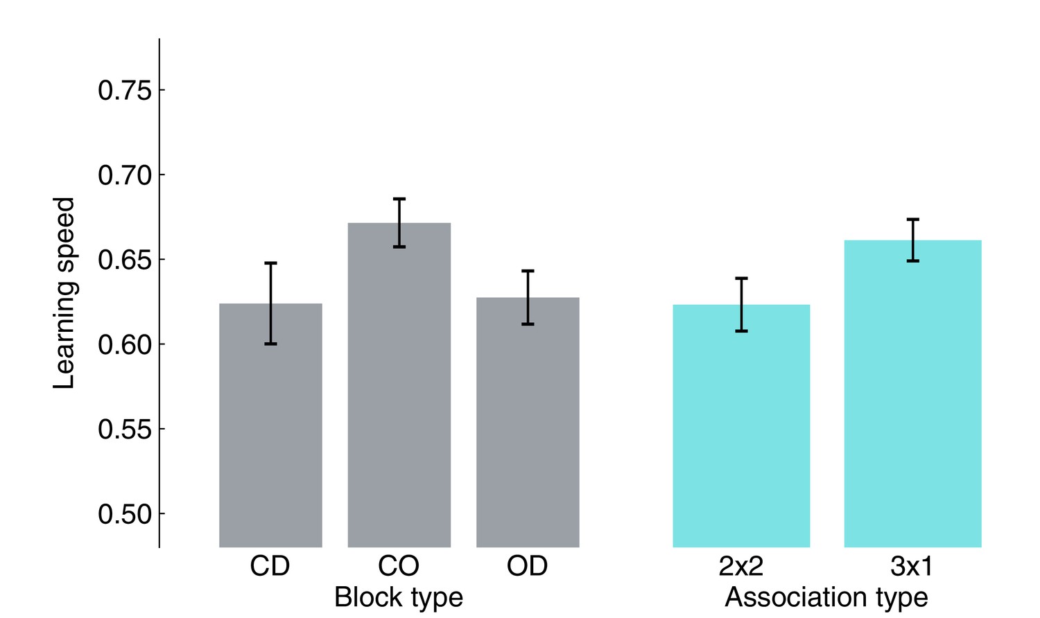
Small (non-significant trends) influence of block/association type on learning speed.
Average learning speed was computed by pooling block-wise learning speed from all participants for each block or association type. None of the pairwise tests survived multiple comparison correction (FDR). Bars represent the population mean, error bars the SEM.
Figure 1—figure supplement 2
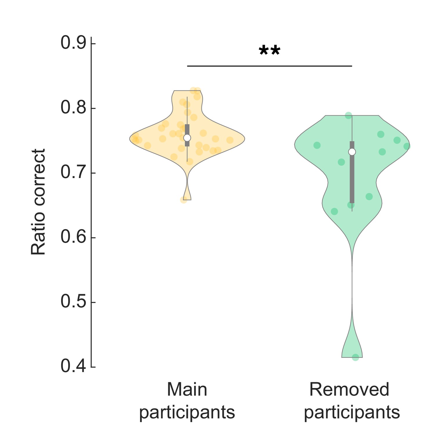
Behaviour analysis of excluded participants.
Excluded participants made more mistakes overall (lower ratio of correct responses). Wilcoxon rank sum test, z = 2.76, p = 0.006.
Figure 2 with 1 supplement
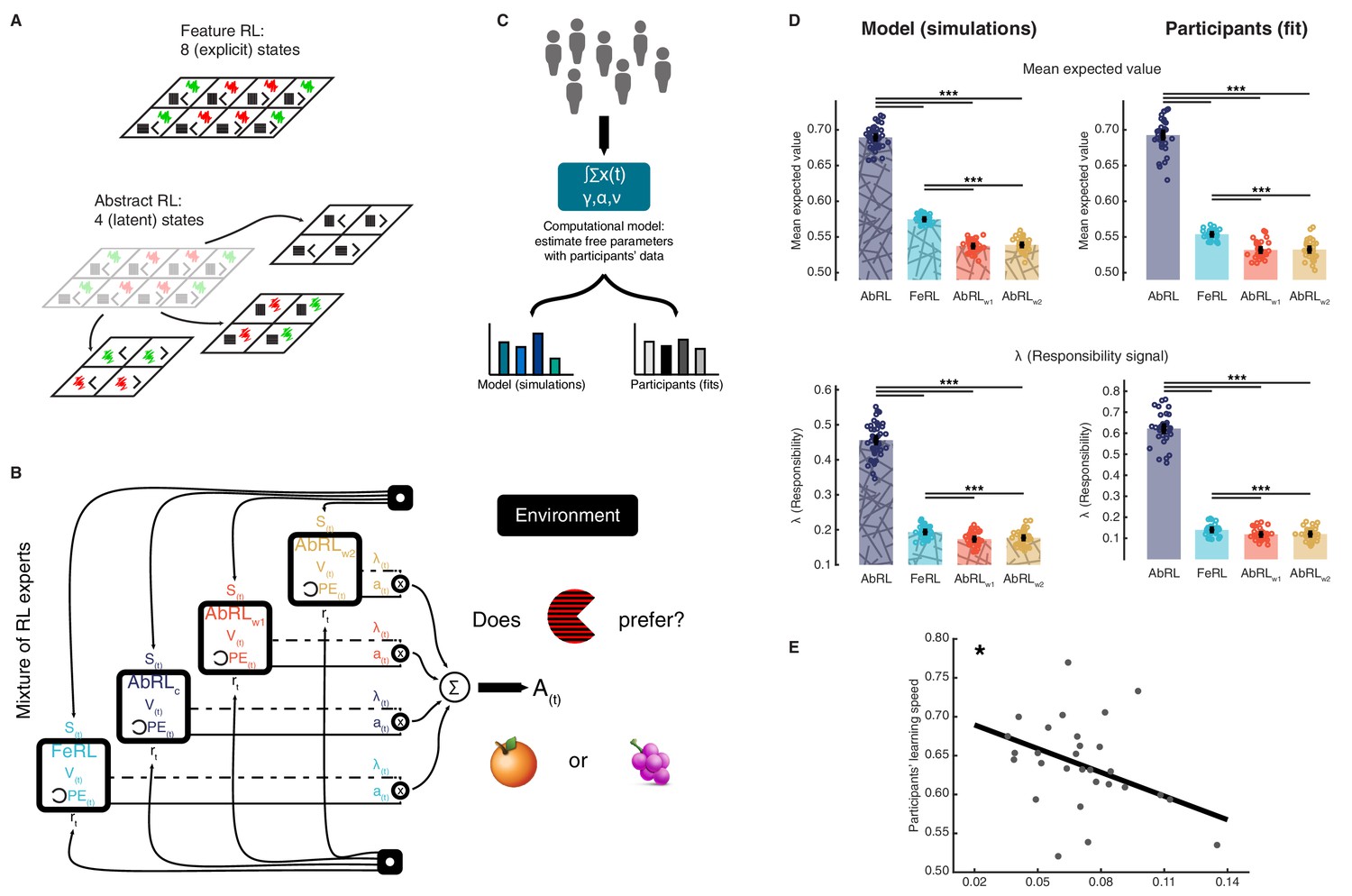
Mixture of reinforcement learning (RL) experts and value computation.
(A) Outline of the representational spaces of each RL algorithm comprising the mixture-of-experts architecture. (B) Illustration of the model architecture. See Methods for a formal description of the model. All experts had the same number of hyperparameters: the learning rate α (how much the latest outcome affected agent beliefs), the forgetting factor γ (how much prior RPEs influenced current decisions), and the RPE variance v, modulating the sharpness with which the mixture-of-expert RL model should favour the best performing algorithm in the current trial. (C) The approach used for data analysis and model simulation. The model was first fitted to participant data with Hierarchical Bayesian Inference (Piray et al., 2019). Estimated hyperparameters were used to compute value functions of participant data, as well as to generate new, artificial choice data and to compute simulated value functions. (D) Averaged expected value across all states for the chosen action in each RL expert, as well as responsibility signal for each model. Left: simulated data, right: participant empirical data. Dots represent individual agents (left) or participants (right). Bars indicate the mean and error bars depict the SEM. Statistical comparisons were performed with two-sided Wilcoxon signed rank tests. ***p<0.001. AbRL: Abstract RL, FeRL: Feature RL, AbRLw1: wrong-1 Abstract RL, AbRLw2: wrong-2 Abstract RL. (E) RPE variance was negatively correlated with learning speed (outliers removed, N = 29). Dots represent individual participant data. The thick line shows the linear regression fit. The experiment was conducted once (n = 33 biologically independent samples), * p<0.05.
-
Figure 2—source data 1
Csv: panel D, mean expected value, model.
- https://cdn.elifesciences.org/articles/68943/elife-68943-fig2-data1-v2.csv
-
Figure 2—source data 2
Csv: panel D, mean expected value, subjects.
- https://cdn.elifesciences.org/articles/68943/elife-68943-fig2-data2-v2.csv
-
Figure 2—source data 3
Csv: panel D, lambda, model.
- https://cdn.elifesciences.org/articles/68943/elife-68943-fig2-data3-v2.csv
-
Figure 2—source data 4
Csv: panel D, lambda, subjects.
- https://cdn.elifesciences.org/articles/68943/elife-68943-fig2-data4-v2.csv
-
Figure 2—source data 5
Csv: panel E.
- https://cdn.elifesciences.org/articles/68943/elife-68943-fig2-data5-v2.csv
Figure 2—figure supplement 1

Model comparison (accounting for model complexity).
Mixture-of-Experts RL (MoE-RL), Feature RL (FeRL), and Abstract RL (AbRL) where fit and compared to each other with Hierarchical Bayesian Inference [HBI] (Piray et al., 2019), at the single participant and block level. (A) Percentage of participants in which the target model best fitted the choice data. The percentage was computed for each block separately (in time, block 1, 2, etc.), then averaged. Bars represent the mean, error bars the SEM. (B) Percentage of blocks (all participants and blocks pooled) in which the target model best fitted the choice data. Bars represent the percentage. (C) Block-specific break-down of the number of participants for which the MoE-RL, the FeRL, or the AbRL provided the best fit.
Figure 3 with 4 supplements
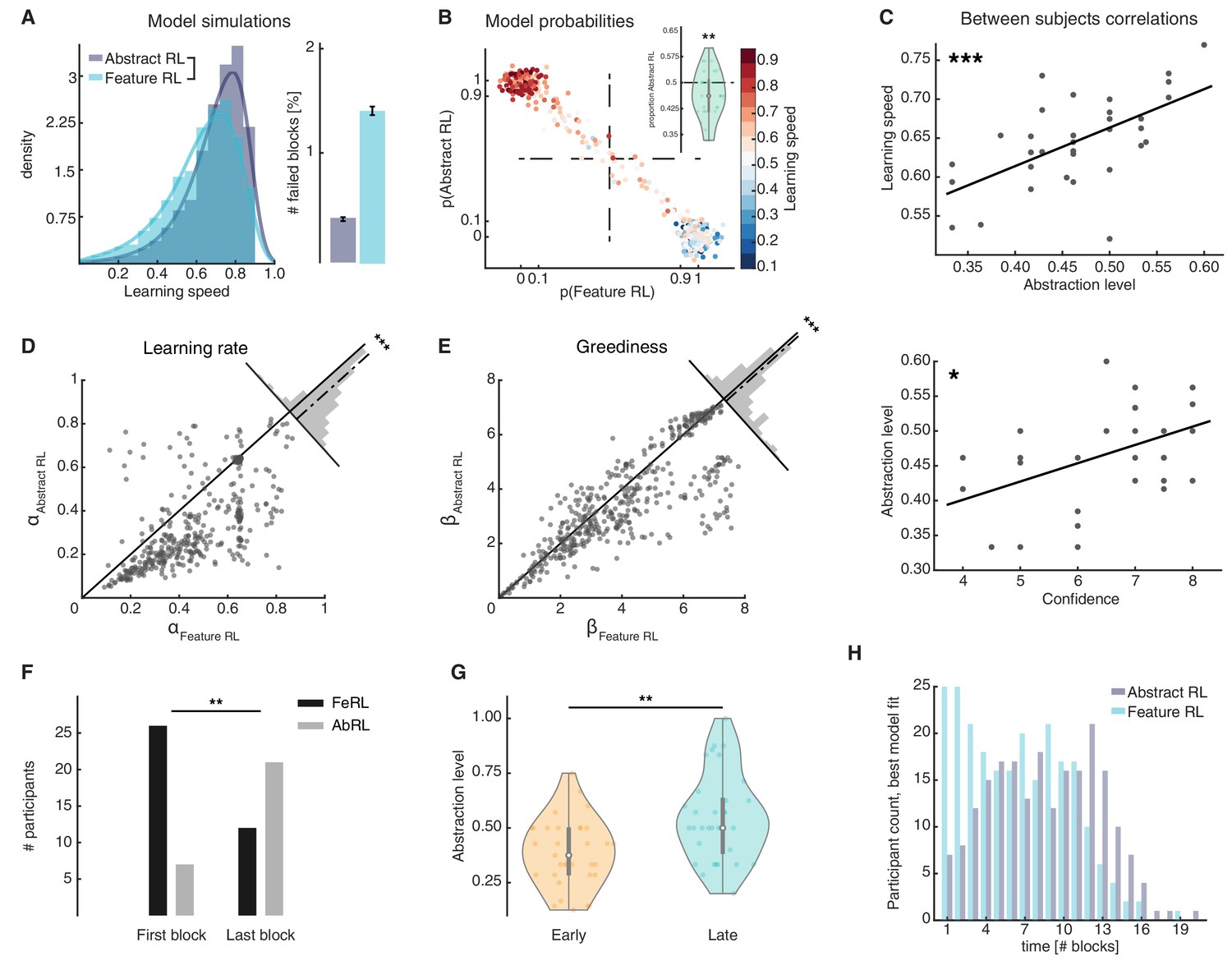
Feature RL vs Abstract RL are related to learning speed and the use of abstraction increases with experience.
(A) Simulated learning speed and % of failed blocks for both Abstract RL and Feature RL. To make simulations more realistic, arbitrary noise was injected into the simulation, altering the state (see Materials and methods). N = 100 simulations of 45 agents. Right plot: bars represent the mean, error bars the SEM. (B) The relationship between the block-by-block, best-fitting model and learning speed of participants. Each dot represents one block from one participant, with data aggregated across all participants. Note that some dots fall beyond p=one or p=0. This effect occurs because dots were scattered with noise in their x-y coordinates for better visualisation. (C) Between participant correlations. Top: abstraction level vs learning speed. The abstraction level was computed as the average over all blocks completed by a given participant (code: Feature RL = 0, Abstract RL = 1). Bottom: confidence vs abstraction level. Dots represent individual participants (top: N = 33, bottom: N = 31, some dots are overlapping). (D) Learning rate was not symmetrically distributed across the two algorithms. (E) Greediness was not symmetrically distributed across the two algorithms. For both (D and E), each dot represents one block from one participant, with data aggregated across all participants. Histograms represent the distribution of data around the midline. (F) The number of participants for which Feature RL or Abstract RL best explained their choice behaviour in the first and last blocks of the experimental session. (G) Abstraction level was computed separately with blocks from the first half (early) and latter half (late) session. (H) Participants count for the best fitting model, in each block. The experiment was conducted once (n = 33 biologically independent samples), * p<0.05, ** p<0.01, *** p<0.001.
-
Figure 3—source data 1
Csv: panel A left, model simulations histogram of learning speed.
- https://cdn.elifesciences.org/articles/68943/elife-68943-fig3-data1-v2.csv
-
Figure 3—source data 2
Csv: panel A right, model simulations % failed blocks.
- https://cdn.elifesciences.org/articles/68943/elife-68943-fig3-data2-v2.csv
-
Figure 3—source data 3
Csv: panel B, scatter plot of model probabilities.
- https://cdn.elifesciences.org/articles/68943/elife-68943-fig3-data3-v2.csv
-
Figure 3—source data 4
Csv: panel B, violin plot of proportion Abstract RL.
- https://cdn.elifesciences.org/articles/68943/elife-68943-fig3-data4-v2.csv
-
Figure 3—source data 5
Csv: panel C.
- https://cdn.elifesciences.org/articles/68943/elife-68943-fig3-data5-v2.csv
-
Figure 3—source data 6
Csv: panel D.
- https://cdn.elifesciences.org/articles/68943/elife-68943-fig3-data6-v2.csv
-
Figure 3—source data 7
Csv: panel E.
- https://cdn.elifesciences.org/articles/68943/elife-68943-fig3-data7-v2.csv
-
Figure 3—source data 8
Csv: panels F and G.
- https://cdn.elifesciences.org/articles/68943/elife-68943-fig3-data8-v2.csv
-
Figure 3—source data 9
csv: panel H.
- https://cdn.elifesciences.org/articles/68943/elife-68943-fig3-data9-v2.csv
Figure 3—figure supplement 1
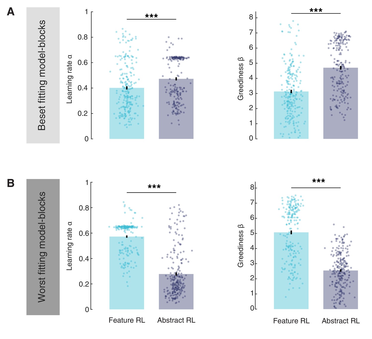
Comparison of learning rate α and greediness β in Feature RL and Abstract RL best-fitting and worst-fitting blocks.
(A) The comparison was done across blocks derived from the model that provided a better fit. Here, the learning rate and greediness in Feature RL blocks was lower than in Abstract RL blocks. Statistical comparisons were performed with Wilcoxon rank-sum two-sided tests. Learning rate: z = −3.88, p = 0.0001; Greediness: z = −8.69, p = 3.5x10⁻¹⁸. (B) The comparison was done across blocks derived from the model that provided a worse fit. The pattern of results reversed, with lower learning rate and greediness for the Abstract RL model. Statistical comparisons were performed with Wilcoxon rank-sum two-sided tests. Learning rate: z = 13.65, p = 2x10−42; greediness: z = 12.91, p = 4.1x10−38. This discrepancy is likely due to the fact that in the blocks in which Abstract RL fits best the data, Feature RL would have very high learning rates / greediness to accommodate behaviour within fewer trials. Conversely, because the blocks in which Feature RL fits the data best also tend to have learning speed (more trials taken to complete), Abstract RL must display much lower learning speeds since the horizon is longer (but with few states). Bars correspond to the mean, error bars the SEM.
Figure 3—figure supplement 2
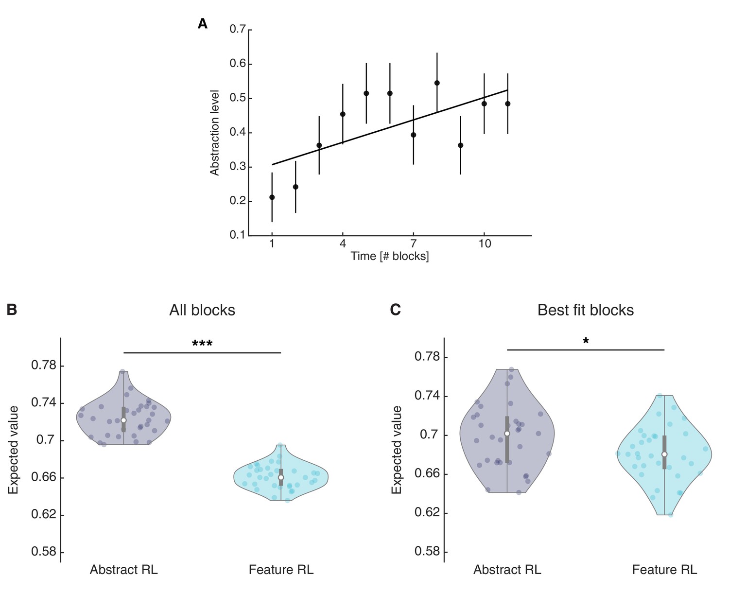
Abstraction index for single blocks and expected value for the chosen action in Abstract RL and Feature RL.
(A) Abstraction index was computed by allocating a value of 0 to blocks labelled as ‘Feature RL’ and one to blocks labelled as ‘Abstract RL’, for each participant. This was done for the first 11 blocks, which were completed by all participants. The plot indicates that, at the group level, there was a tendency towards increasingly higher abstraction later in time. Each dot represents the population mean, error bars the SEM. The least square line fit, robust regression, and p-value were computed on the 11 mean data points. Robust regression slope = 0.022, t31 = 2.34, p = 0.044. (B) Mean expected value computed from all blocks, when fitted with either Abstract RL or Feature RL. (C) Mean expected value computed from the best fitting algorithms on a given block. That is, Abstract RL (resp. Feature RL) refers to the expected value for the chosen action in blocks where Abstract RL (resp. Feature RL) was the best fitting algorithm. Two (B) and one (C) outliers were removed. Each coloured dot represents the average expected value for the chosen options for a single participant - in either Abstract RL (grey) or Feature RL (cyan). Shaded areas represent the density plot, central white dot the median, the dark central bar the interquartile range, and thin dark lines the lower and upper adjacent values. (B) two-sided t-test, t30 = 35.66, p = 4.03x10⁻²⁶. (C) two-sided t-test, t31 = 2.31, p = 0.028.
Figure 3—figure supplement 3
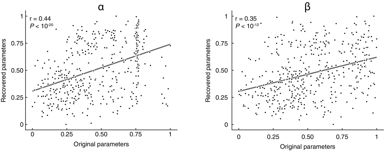
Parameter recovery.
We first simulated choice data through the models, using the best-fitting parameters. Simulated data was then fed again to the fitting procedure using HBI, separately for each model, in the presence of noise (the update was sometimes not done for the real, correct state but rather for an alternative, random state). Parameters were recovered for each participant, block, and model. Recovered and original parameter values were then pooled across the models and plotted. Values were normalized in the interval [0, 1] for visualisation purposes (note that the normalisation does not affect the strength of the correlation).
Figure 3—figure supplement 4
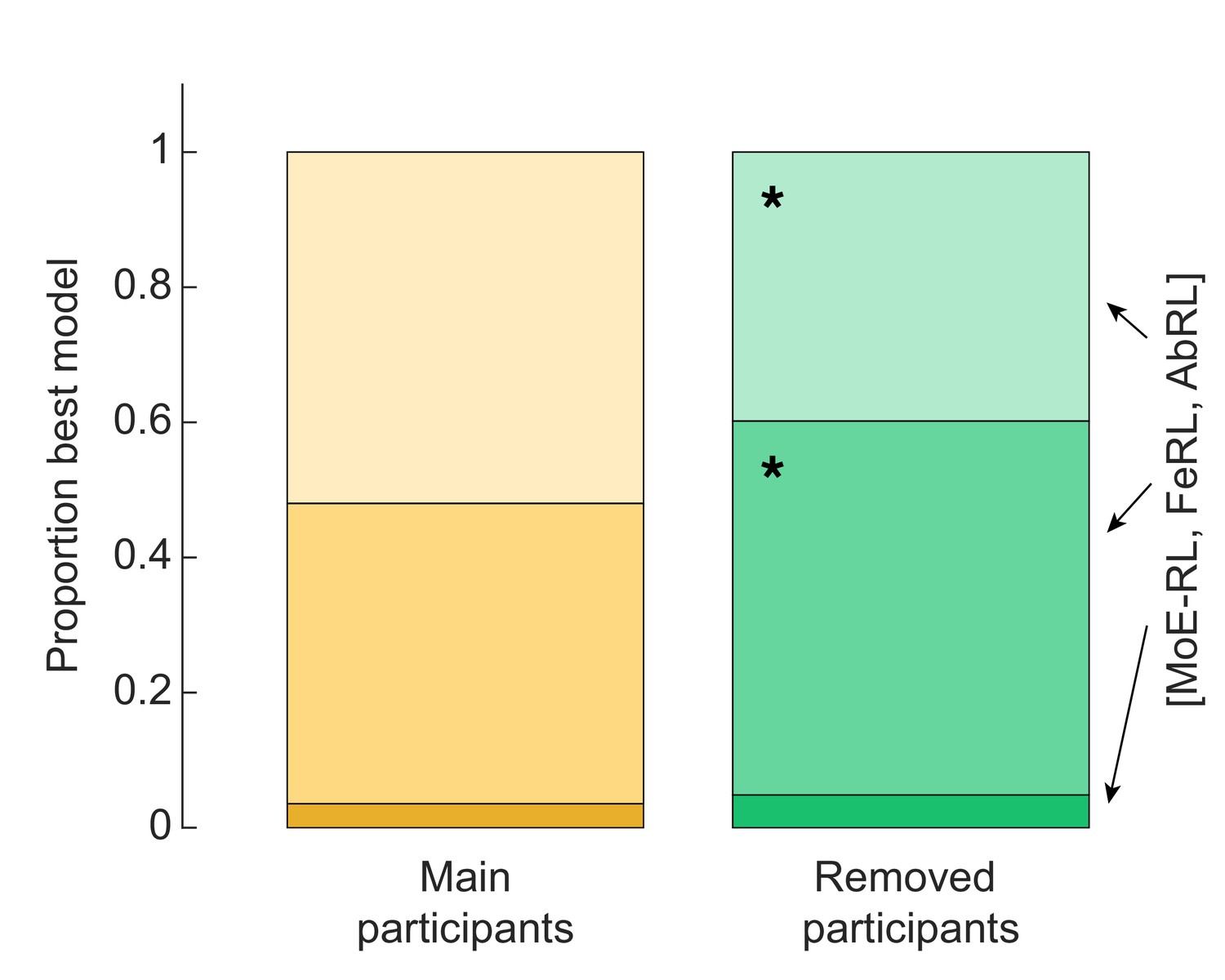
Strategy analysis of excluded participants.
Excluded participants tended to rely more often on a Feature RL strategy. Binomial test Feature RL: base rate of 0.44 calculated from the main participants group, P(57|103) = 0.029. Binomial test Abstract RL: base rate of 0.52 calculated from the main participants group, P(41|103) = 0.014.
Figure 4 with 2 supplements
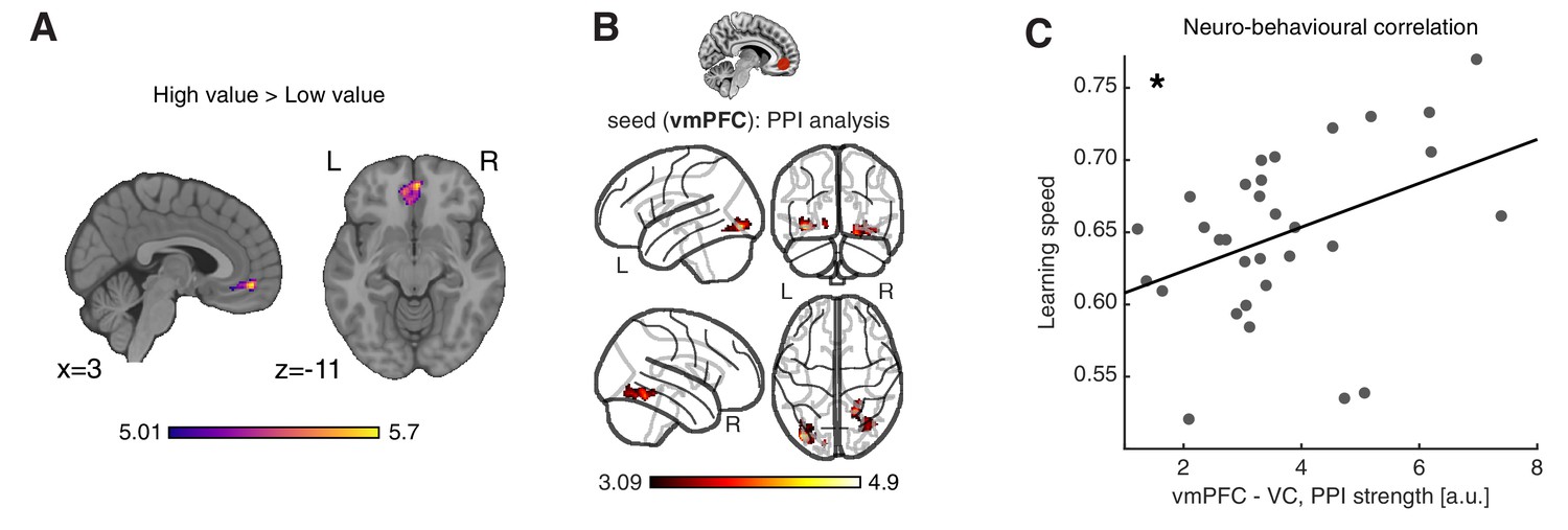
Neural substrates of value construction during learning.
(A) Correlates of anticipated value at pacman stimulus presentation time. Trials were labelled according to a median split of the expected value for the chosen action, as computed by the best fitting model, Feature RL or Abstract RL, at the block level. Mass univariate analysis, contrast ‘High-value’ > ‘Low-value’. vmPFC peaks at [2 50 -10]. The statistical parametric map was z-transformed and plotted at p(FWE) < 0.05. (B) Psychophysiological interaction, using as seed a sphere (radius = 6 mm) centred around the participant-specific peak voxel, constrained within a 25 mm sphere centred around the group-level peak coordinate from contrast in (A). The statistical parametric map was z-transformed and plotted at p(fpr) < 0.001 (one-sided, for positive contrast - increased coupling). (C) The strength of the interaction between the vmPFC and VC was positively correlated with participant’s ability to learn block rules. Dots represent individual participant data points, and the line is the regression fit. The experiment was conducted once (n = 33 biologically independent samples), * p<0.05.
-
Figure 4—source data 1
Csv: panel C.
- https://cdn.elifesciences.org/articles/68943/elife-68943-fig4-data1-v2.csv
Figure 4—figure supplement 1
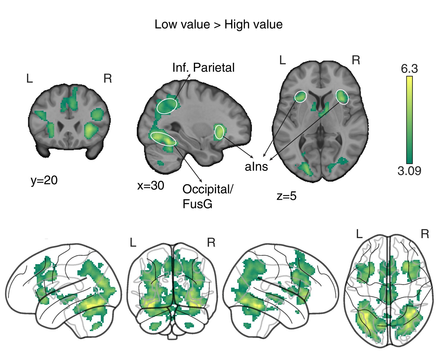
‘Low value’ > ‘High value’ GLM contrast.
Neural correlates of (predicted) low value at visual stimulus presentation time. Trials were labelled according to a median split of the expected value for the chosen option as computed by the best fitting model, at the participants and block level. The statistical parametric map was z-transformed, and false-positive means of cluster formation (fpr) correction was applied. p(fpr) < 0.001, Z > 3.09.
Figure 4—figure supplement 2
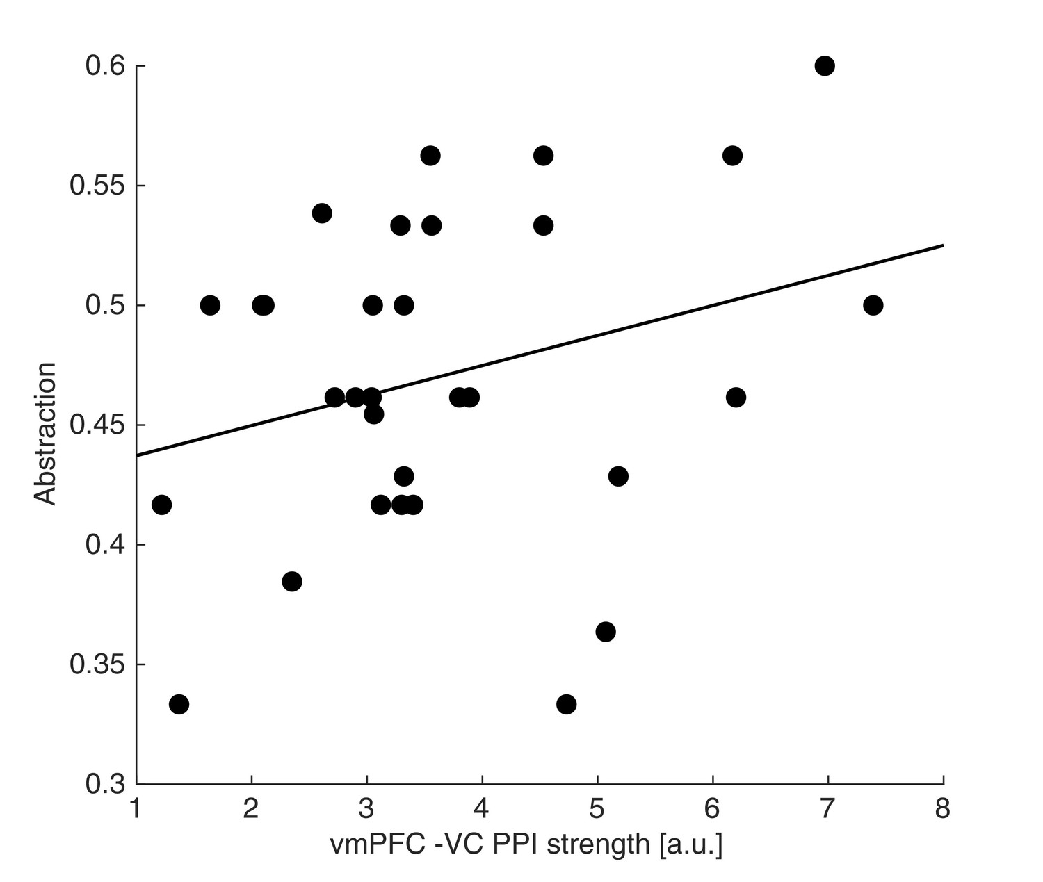
Neuro-behavioural correlation between VC-vmPFC coupling and abstraction.
The strength of the interaction between the vmPFC and VC showed a weak positive association with the abstraction level across participants. Dots represent individual participant data points, and the line is the regression fit. The experiment was conducted once (n = 33 biologically independent samples), robust regression fit: N=31, slope = 0.013, t31 = 1.56, p = 0.065 (one-sided).
Figure 5 with 3 supplements

Neural substrate of abstraction.
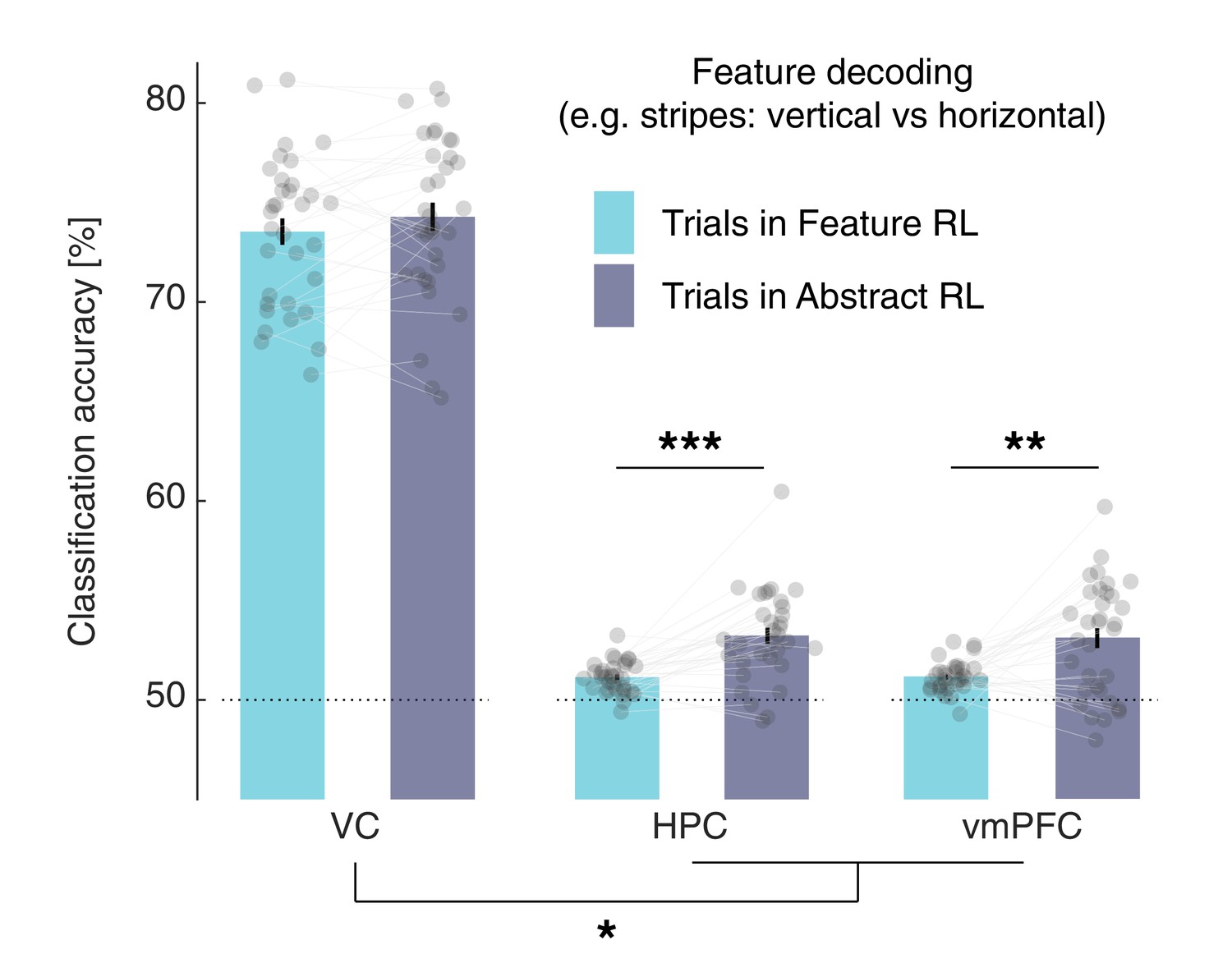
(A) Regions of interest for univariate and multivariate analyses. The HPC was defined through automated anatomical labelling (FreeSurfer). The vmPFC was functionally defined as the cluster of voxels found with the orthogonal contrast ‘High value’ > ‘Low value’, at P(unc) < 0.0001. (B) ROI activity levels corresponding to each learning mode were extracted from the contrasts ‘Feature RL’ > ‘Abstract RL’, and ‘Abstract RL’ > ‘Feature RL’. Coloured bars represent the mean, and error bars the SEM. (C) Multivariate (decoding) analysis in three regions of interest: VC, HPC, vmPFC. Binary decoding was performed for each feature (e.g. colour: red vs green), by using trials from blocks labelled as Feature RL or Abstract RL. Colour bars represent the mean, error bars the SEM, and grey dots represent individual data points (for each individual, taken as the average across all three classifications, i.e., of all features). Results were obtained from leave-one-run-out cross-validation. The experiment was conducted once (n = 33 biologically independent samples), * p<0.05, ** p<0.01. (D) Classification was performed for each feature pair (e.g. colour: red vs green), separately for blocks in which the feature in question was relevant or irrelevant to the block’s rule. The statistical map represents the strength of the reduction in accuracy between trials in which the feature was relevant compared to irrelevant, averaged over all features and participants. (E) Classification of the rule (2x2 blocks only). For each participant, classification was performed as fruit 1 vs fruit 2. In (D–E ), statistical parametric maps were z-transformed, false-positive means of cluster formation (fpr) correction was applied. p(fpr) < 0.01, Z > 2.33.
-
Figure 5—source data 1
Csv: panel B.
- https://cdn.elifesciences.org/articles/68943/elife-68943-fig5-data1-v2.csv
-
Figure 5—source data 2
Csv: panel C.
- https://cdn.elifesciences.org/articles/68943/elife-68943-fig5-data2-v2.csv
Figure 5—figure supplement 1
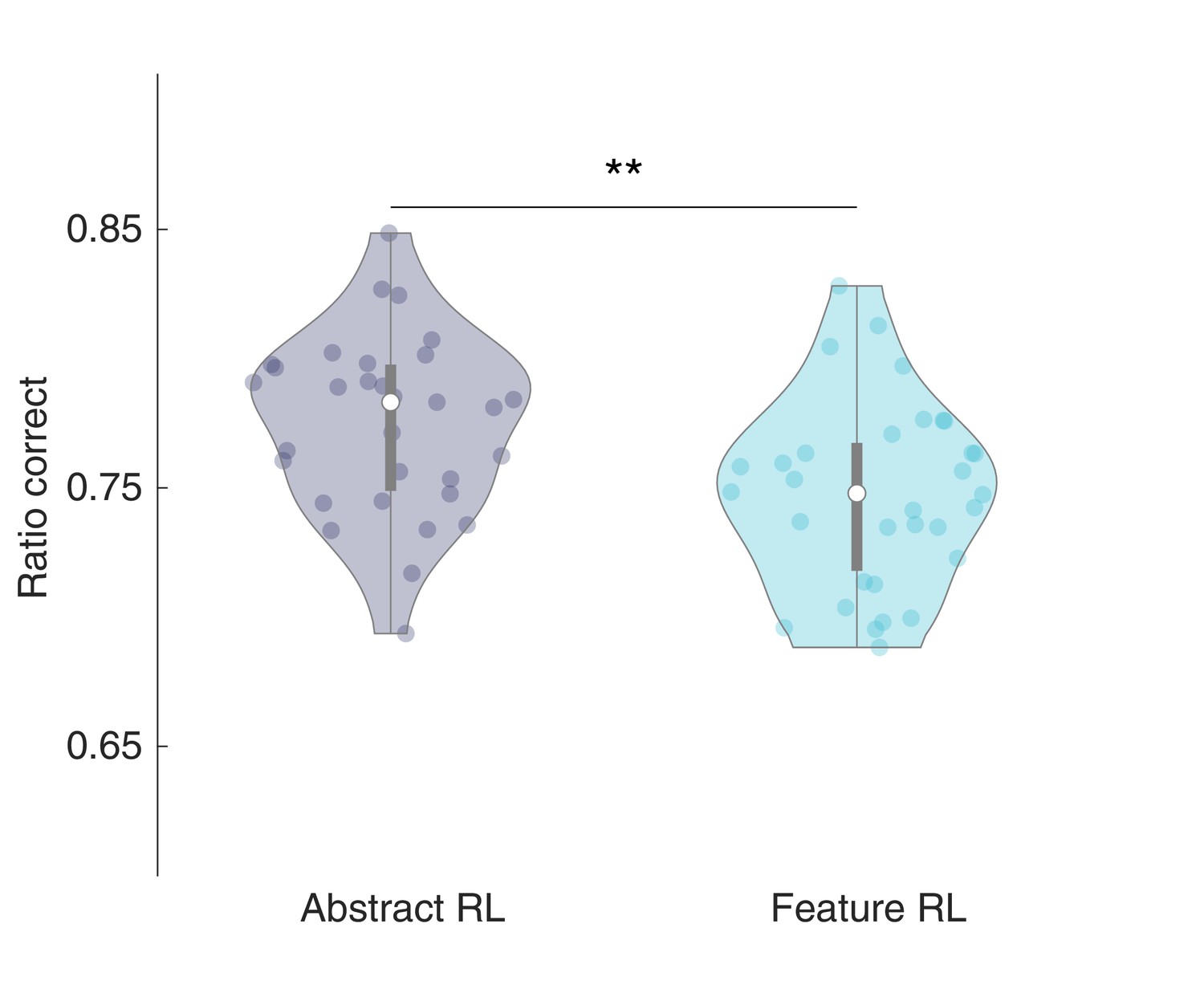
Ratio correct in Feature RL and Abstract RL.
Mean ratio of correct choices total choices, for trials labelled as Feature RL and Abstract RL (i.e., the best fitting algorithm on a given block). A total of three (Abstract RL: two, Feature RL: one) outliers were removed. Each coloured dot represents the average across selected blocks for a single participant - in either Abstract RL (grey) or Feature RL (cyan). Shaded areas represent the density plot, central white dot the median, the dark central bar the interquartile range, and thin dark lines the lower and upper adjacent values. Two-sided t-test, t29 = 3.23, p = 0.003 (**).
Figure 5—figure supplement 2
Value functions correlations and reaction time differences in Feature RL and Abstract RL trials.
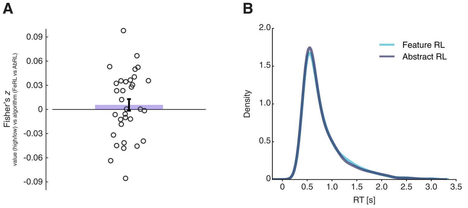
(A) Fisher-transformed coefficients (Spearman ρ) of the correlation between high/low value and Feature RL / Abstract RL across trials. The coloured bar represents the population mean, the error bar the SEM, and dots individual participants’ data. The two labels used in the main GLM were uncorrelated. Wilcoxon sign rank test against median 0, z = 0.72, p = 0.47. (B) Reaction time (RT) data pooled over all participants for trials in blocks labelled as ‘Feature RL’ or ‘Abstract RL’. RT was not significantly different between the two strategies. Wilcoxon sign rank test between the two distributions, z = 1.48, p = 0.14.
Figure 5—figure supplement 3
K-fold cross-validation in feature decoding, using Feature RL and Abstract RL trials separately.
The split of the data in training and test subsets was done (N=20) by randomly selecting 80% of the Nmin trials across the two levels of the target feature and the two conditions (Feature RL and Abstract RL). Thus, in each fold, the same number of trials for each feature and condition was used to train the classifier, avoiding possible accuracy confounds due to varying numbers of trials used for training. As in the primary analysis reported in the main text, classification accuracy was significantly higher in Abstract RL compared with Feature RL trials in both the HPC and vmPFC (two-sided Wilcoxon signed rank test, HPC: z = −4.21, p(FDR) < 0.001, vmPFC: z = −3.15, p(FDR) = 0.002), but not in VC (z = −1.30, p(FDR) = 0.20). The difference in feature decodability was significantly larger in the HPC and vmPFC compared to the VC (LMEM model ‘y ~ ROI + (1|participants)’, y: difference in decodability, t97 = 2.52, p = 0.013).
Figure 6 with 1 supplement

Artificially adding value to a feature’s neural representation.
(A) Schematic diagram of the follow-up multivoxel neurofeedback experiment. During the neurofeedback procedure, participants were rewarded for increasing the size of a disc on the screen (max session reward 3000 JPY). Unbeknownst to them, disc size was changed by the computer program to reflect the likelihood of the target brain activity pattern (corresponding to one of the task features) measured in real time. (B) Blocks were subdivided based on the feature targeted by multivoxel neurofeedback as ‘relevant’ or ‘irrelevant’ to the block rules. Scatter plots replicate the finding from the main experiment, with a strong association between Feature RL / Abstract RL and learning speed. Each coloured dot represents a single block from one participant, with data aggregated from all participants. (C) Abstraction level was computed for each participant from all blocks belonging to: (1) left, the latter half of the main experiment (as in Figure 3G, but only selecting participants who took part in the multivoxel neurofeedback experiment); (2) centre, post-neurofeedback for the ‘relevant’ condition; (3) right, post-neurofeedback for the ‘irrelevant’ condition. Coloured dots represent participants. Shaded areas indicate the density plot. Central white dots show the medians. The dark central bar depicts the interquartile range, and dark vertical lines indicate the lower and upper adjacent values. (D) Bootstrapping the difference between model probabilities on each block, separately for ‘relevant’ and ‘irrelevant’ conditions. The experiment was conducted once (n = 22 biologically independent samples), * p<0.05, *** p<0.001.
-
Figure 6—source data 1
Csv: panel B, irrelevant blocks.
- https://cdn.elifesciences.org/articles/68943/elife-68943-fig6-data1-v2.csv
-
Figure 6—source data 2
Csv: panel B, relevant blocks.
- https://cdn.elifesciences.org/articles/68943/elife-68943-fig6-data2-v2.csv
-
Figure 6—source data 3
Csv: panel C.
- https://cdn.elifesciences.org/articles/68943/elife-68943-fig6-data3-v2.csv
-
Figure 6—source data 4
Csv: panel D.
- https://cdn.elifesciences.org/articles/68943/elife-68943-fig6-data4-v2.csv
Figure 6—figure supplement 1
Neurofeedback experiment results.
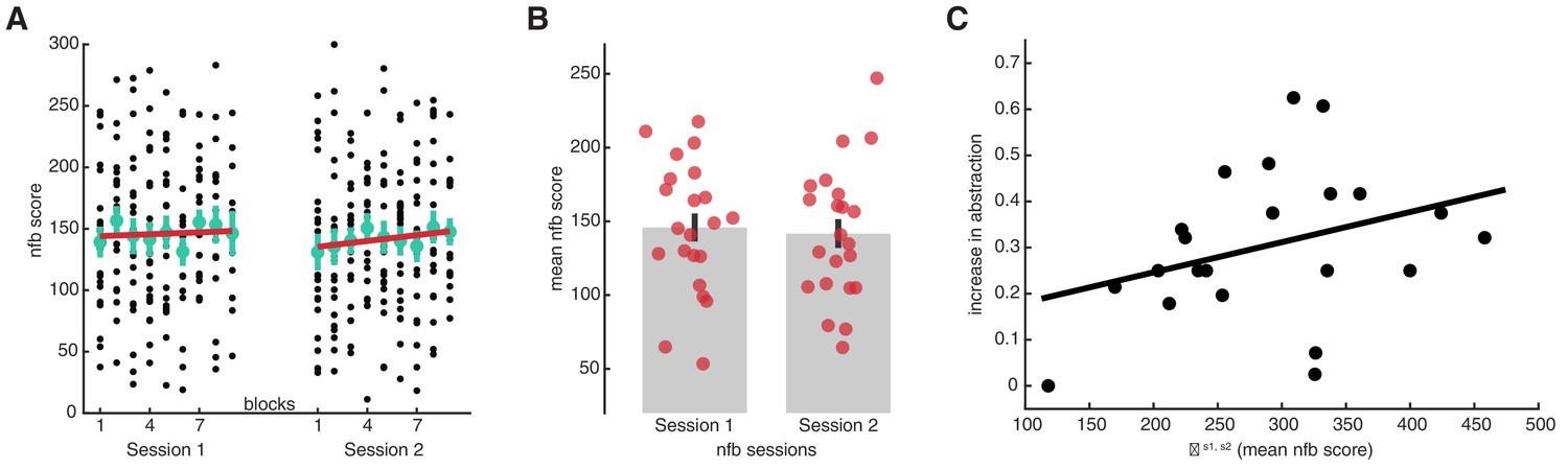
(A) Neurofeedback (nfb) scores from each block of training, for sessions 1 and 2. Black dots represent data from individual participants, as the score obtained within a block of nfb training. Large green dots represent the mean, and the error bars the SEM. The red line is a linear fit on the mean data points. Robust regression fits, session 1: slope = 0.75, t7 = 0.60, p = 0.57; session 2: slope = 1.67, t7 = 1.98, p = 0.088. (B) Average nfb scores attained in each session. The red circles represent individual participants, the grey bars group means, and the black error bars the SEM. (C) Correlation between the sum of mean nfb scores (session 1 + session 2) and the subsequent increase in abstraction. The increase in abstraction was calculated as the difference between the abstraction level in the ‘relevant’ blocks and the abstraction level at the beginning of the main learning task. Black circles represent individual participants, and the black line a linear fit. N = 22, Spearman’s rho = 0.39, p = 0.036 (one-sided test for positive correlation). Source data files. Source data files for each figure are available with this manuscript.
Additional files
Download links
A two-part list of links to download the article, or parts of the article, in various formats.
Downloads (link to download the article as PDF)
Open citations (links to open the citations from this article in various online reference manager services)
Cite this article (links to download the citations from this article in formats compatible with various reference manager tools)
Value signals guide abstraction during learning
eLife 10:e68943.
https://doi.org/10.7554/eLife.68943


