Figures and data in Mechanical vibration patterns elicit behavioral transitions and habituation in crawling Drosophila larvae | eLife

Figures
Additional files

7 figures and 3 additional files

Figures

Figure 1

Download asset Open asset

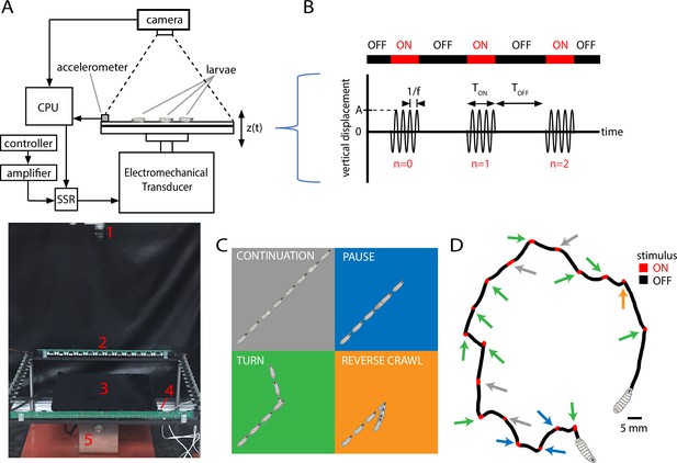
Vibration stimulus delivery and avoidance behavior classification.

(A) Top: schematic of the experimental setup, where larvae crawl on a vertically vibrated agar gel supported by aluminum and steel plates. An electromechanical transducer provides vibration, while a CCD camera records 2D crawling of $\approx 20$ red-light-illuminated animals simultaneously. See ‘Methods and materials’ for details. Bottom: photograph of the experimental setup, with red numbering labeling (1) camera, (2) LED array, (3) crawling substrate, (4) accelerometer, and (5) mechanical shaker. (B) Stimulus pattern in a typical experiment. Beginning at time $t = 0$ , pulses of sinusoidal vibration are delivered for a duration of $T_{O N}$ , and repeated at times $t = n (T_{O F F} + T_{O N}) = n T$ , where $n$ is an integer referring to nth application of the stimulus. The initial vibration is referred to as the $n = 0$ stimulus, the next as $n = 1$ , etc. Vibration strength is described by the frequency $f$ and the peak (dimensionless) acceleration $Γ$ . In the top horizontal bar, red indicates stimulus ON, and black indicates stimulus OFF. (C) Schematic of four behavioral responses to non-nociceptive vibration: continuation (gray), pause (blue), turn (green), and reverse (orange). In each illustration, the larva crawls forward from the bottom left, and a stimulus is delivered in the center. Pictures in the sequence are equally spaced in time. (D) Representative trajectory of a single larva crawling for 300 s during a vibration experiment ( $f = 500$ Hz, $Γ = 2$ , $T_{O N} = 10$ s, $T_{O F F} = 20$ s). The four behaviors are indicated by arrows matching the behavior’s color from (C). The regions with the stimulus ON appear shorter than the OFF segments because larvae come to a stop before adjusting direction, and this can take at least several seconds.

Figure 1—source code 1 Code from MATLAB that determines the behavioral state of crawling larvae. The program uses input data from the MAGAT Analyzer software (Gershow et al., 2012).: https://cdn.elifesciences.org/articles/69205/elife-69205-fig1-code1-v1.zip
Download elife-69205-fig1-code1-v1.zip

Figure 2

Download asset Open asset

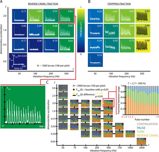
Fractional strong and weak behavioral responses depend on vibration strength.

(A) Reversal behavior heat map. Vibration parameters were $T_{O N} = 10$ s, $T_{O F F} = 20$ s, with $Γ$ ranging from $0 - 2$ and frequency between 50 and 500 Hz. $F_{0, R E V}$ , the fraction of larvae that reverse crawl after the first ( $n = 0$ ) vibration pulse is printed for each $f - Γ$ square region, alongside graphs of $F_{R E V} (t)$ , averaged over all experiments. Color indicates the $F_{0, R E V}$ value. All graphs have the same scale in $F$ and $t$ . Each ( $f, Γ$ ) result is based on five experiments, each with $\approx 20$ larvae (total 1300 animals), and lasting 600 s. Note that the $f$ and $Γ$ axes are not on a linear scale. Uncertainties in $F_{0, R E V}$ are not listed, but are $< 0.001$ for all values. (B) Stopping behavior heat map. From the same experiments as (A), but considering $F_{S T O P}$ , the fraction of larvae showing any avoidance behavior (pause, turn, or reversal). As vibration strength increases (along either the $f$ or $Γ$ axes), the fraction of avoidant larvae increases. (C) Inset: fractional deployment of the behavioral repertoire during habituation. $F_{R E V}$ (orange), $F_{T U R N}$ (green), $F_{P A U S E}$ (blue), and $F_{C O N T}$ (gray) during a 3-s window after pulse initiation, as a function of the pulse number $n$ . Over time the stronger avoidance behavior diminishes in favor of weaker avoidance and nonavoidance. $Γ = 2$ , $f = 500$ Hz. Larger graph: behavioral repertoire over a range of vibration space. Fractional use of behaviors as a function of vibration pulse number ( $n$ ) for repeated vibrations ( $T_{O N} = 10$ s, $T_{O F F} = 30$ s), for many specific $f$ , $Γ$ combinations. Each experimental condition is represented by a $F$ vs. $n$ plot, and the response of 100 larvae is averaged, for a total of 2900 animals. Lines bridging adjacent graphs indicate whether the two sets of vibration conditions induce a significantly different reverse crawl probability following the $n = 0$ pulse, colored either yellow for p<0.05 and black for p>0.05 (Fisher’s exact test). Red dots on the graphs indicate a reverse crawl probability significantly greater than the baseline (zero vibration) response probability (Fisher’s exact test).

Figure 3

Download asset Open asset

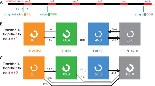
Habituation to repeated pulses is an essentially one-way process for individuals.

(A) Schematic of the stimulus pattern and example analysis. The stimulus consisted of vibration ( $f = 500$ Hz, $Γ = 2$ ) with repeated pulses of width $T_{O N} = 10$ s, repeated after $T_{O F F} = 20$ s. The behavior of each individual, in the 3 s following the onset of each vibration pulse, was assigned to one of four categories: reverse crawl (orange), turn (green), pause (blue), or continuation (gray). In the example shown, a larva reverse crawls in response to the $n = 0$ pulse, then turns in response to the next, and continues in response to the $n = 5$ pulse. (B, C) Behavioral transitions during repeated stimuli for individual larvae. For a given behavior observed in response to pulse $n$ , the arrows represent the percentage of larvae that exhibit each of the four behaviors in response to pulse $n + 1$ (B) or $n + 5$ (C). White circular arrows represent repeating the same behavior, and the thickness of the black arrows is proportional to the fraction of animals that make the respective transition. The sum of the repeat arrows and all outgoing arrows is 100 for each behavior. Larvae were observed in five separate experiments, for a total of 107 animals making $\approx 1800$ behavioral transitions.

Figure 4

Download asset Open asset

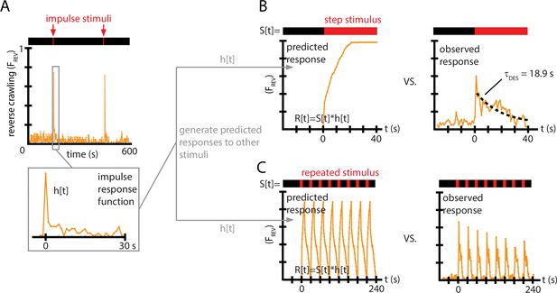
Impulse response experiments show that avoidance response to vibration is nonlinear and adaptive.

(A) The fraction of larvae performing reverse crawling ( $F_{R E V}$ (t)) while exposed to very short bursts of strong vertical vibration ( $f = 500$ Hz, $Γ = 2$ , $T_{O N} = 1$ s, $T = 300$ s). Inset shows a time-expanded view of the response, labeled as $h [t]$ to denote the impulse response function (IRF) used to make predictions for other stimulus inputs. (B) Avoidant response ( $F_{R E V}$ ) to continuous vibration, as predicted by a linear, time-invariant (LTI) model using the impulse responses $h [t]$ from (A) (left), and as observed empirically (right) (i.e., $T_{O F F} = 0$ ) with $f = 500$ Hz and $Γ = 2$ . (C) Avoidant response ( $F_{R E V}$ ) to repeated pulse vibration ( $f = 500$ Hz, $Γ = 2$ , $T_{O N} = 10$ s, $T_{O F F} = 20$ s), as predicted by a linear, LTI model using the impulse responses $h [t]$ from (A) (left), and as observed empirically (right). The LTI calculation fails to predict the empirical behavior due to de-sensitization (B) and slow re-sensitization (C). Each plot is the average from five experiments using 20 larvae each (total 100 animals).

Figure 5

Download asset Open asset

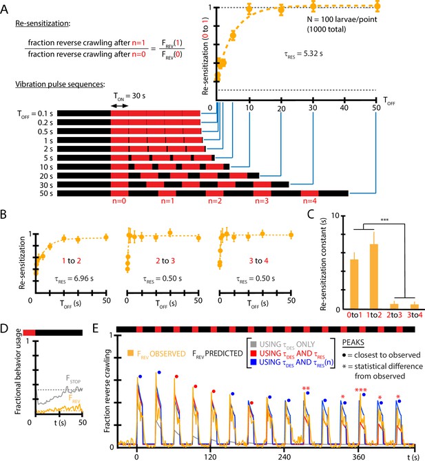
Re-sensitization after removal of mechanical stimulus depends on prior vibration pulses.

(A) Visualization of vibration pulse sequence experiments used to determine re-sensitization to the stimulus. Time $t = 0$ indicates the start of the initial ( $n = 0$ ) vibration pulse period, lasting $T_{O N} = 30$ s (red). The stimulus is removed between pulses for varying amounts of time $T_{O F F}$ . Recovery of sensitization is determined for each pulse $n$ by computing the ratio $F_{n, R E V}$ to $F_{n - 1, R E V}$ , normalized to account for incomplete recovery for short $T_{O F F}$ times. Lower dashed line indicates baseline (no stimulus) reversal fraction. (B) Re-sensitization as a function of the time $T_{O F F}$ , determined for the $n = 1$ , $n = 2$ , $n = 3$ , and $n = 4$ pulses. Vibration intensity was $f = 500$ Hz, $Γ = 2$ . Each data point is the average from five experiments of $\approx 20$ animals each, for a total of 1000 larvae from 50 experiments. Error bars are SEM. (C) Re-sensitization time constants as a function of vibration pulse number $n$ . $τ_{r e s}$ was determined from fits of the data in (A) and (B) (Equation 4). After two vibration pulses, the re-sensitization is significantly faster (***p<0.001, Student’s t-test). (D) Behavioral response to the ON→OFF stimulus transition: $F_{R E V} (t)$ and $F_{S T O P} (t)$ , where $t = 0$ indicates the stimulus OFF transition. $F_{R E V}$ is unaffected. Vibration conditions ( $f = 500$ Hz, $Γ = 2$ , $T_{O N} = 50$ s, $T_{O F F} = 30$ s). Data points are the average of $F_{S T O P}$ (gray) and $F_{R E V}$ (orange) up to the $n = 9$ pulse. Dashed lines indicate the baseline behavior fractions while the stimulus is ON. (E) Comparison of habituation models with $τ_{d e s}$ , $τ_{r e s}$ , and $τ_{r e s}$ vs. $n$ dependence (blue) to empirical strong avoidance behavior $F_{R E V} (t)$ (orange), as well as more limited models with only $τ_{d e s}$ (gray) or only $τ_{d e s}$ and $τ_{r e s}$ (red). Colored circle markers above each peak indicate which model was closest to the empirical peak value, while * symbols indicate whether the model peak value was significantly different than the empirical peak value (Fisher’s exact test, *p<0.05, **p<0.01, ***p<0.001, gray trace not included).

Figure 5—source code 1 Code in Igor Pro for performing fits to determine desensitization and re-sensitization time constants from reversal count data.: https://cdn.elifesciences.org/articles/69205/elife-69205-fig5-code1-v1.zip
Download elife-69205-fig5-code1-v1.zip

Figure 6

Download asset Open asset

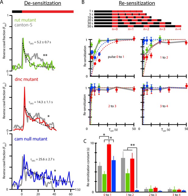
Memory-deficient mutants have distinct habituation and de-habituation time constants.

(A) De-sensitization: reverse crawl behavior usage in response to continuous vibration stimulation. $F_{R E V}$ vs. $t$ (where $t = 0$ marks the vibration onset) for three mutants: rut (green), dnc (red), and cam0 (blue). Gray traces are the Canton-S wild-type response from Figure 4B. Vibrations were $f = 500$ Hz and $Γ = 2$ . Each trace is based on five experiments, with 20 larvae in each. (B) Re-sensitization to vibration following repeated pulses. Top: schematic of experiments performed. Bottom: plots of $F_{n, R E V} / F_{n - 1, R E V}$ vs. $T_{O F F}$ after the nth pulse for rut (green), dnc (red), and cam0 (blue). Gray traces are the Canton-S wild-type response from Figure 5. Vibrations were $f = 500$ Hz and $Γ = 2$ . Each point is based on 5 experiments, with 20 larvae in each, for a total of 75 experiments and $\approx 1500$ larvae. Error bars indicate SEM. (C) Desensitization and Re-sensitization time constants as functions of pulse number $n$ for the same three mutants, based on fits to the data in (B). Error bars indicate SEM. *p<0.05 and **p<0.01.

Figure 7

Download asset Open asset

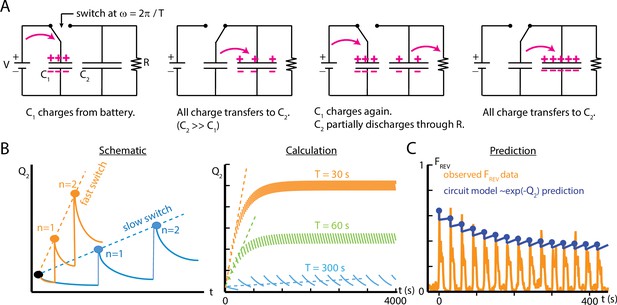
An electric circuit models possible mechanisms for larval habituation.

(A) The capacitor switch circuit, where a small capacitor C₁ is continually charged by a battery $V$ , and discharges to a larger capacitor C₂ each time the switch changes. The charge Q₂ is related to the probability $P$ of observing an external event ( $Q_{2} = - \ln P$ ). (B) Functions $Q_{2} (t)$ created by varying the duration of the charging phase of the circuit, $T$ , while holding the circuit elements constant. Left: a visual schematic of such functions. Right: $Q_{2} (t)$ generated by simulating the circuit behavior. In each case, after enough switches, the charge saturates when the charging from C₁ to C₂ balances the charge dissipated through $R$ for each cycle. For values of $T$ much smaller than $R C_{2}$ , this saturation will only occur at a large $n$ . (C) Comparison of the circuit model to empirical data of reverse crawl probability ( $f = 500$ Hz, $Γ = 2$ , $T_{O N} = 10$ s, $T_{O F F} = 20$ s, same data shown in Figure 4C). The circuit values are $V = 1$ , $C_{1} = 1.2$ , $C_{2} = 160$ , $R = 1$ , with the switch operating with period $T = 30$ . The peak values from the circuit model do not significantly differ from the empirical peaks (p>0.05, Fisher’s exact test).

Additional files

Transparent reporting form: https://cdn.elifesciences.org/articles/69205/elife-69205-transrepform1-v1.docx
Download elife-69205-transrepform1-v1.docx
Source code 1 Matlab script, which should be run in the MAGAT Analyzer environment after loading movie files, that determines the behavioral state of crawling larvae, in particular identifying reverse-crawl behavior.: https://cdn.elifesciences.org/articles/69205/elife-69205-code1-v1.zip
Download elife-69205-code1-v1.zip
Source code 2 Functions in Igor Pro that perform fits to larva crawling data, used to extract desensitization and re-sensitization time constants.: https://cdn.elifesciences.org/articles/69205/elife-69205-code2-v1.zip
Download elife-69205-code2-v1.zip

Download links

A two-part list of links to download the article, or parts of the article, in various formats.

Downloads (link to download the article as PDF)

Article PDF

Open citations (links to open the citations from this article in various online reference manager services)

Mendeley

Cite this article (links to download the citations from this article in formats compatible with various reference manager tools)

Alexander Berne
Tom Zhang
Joseph Shomar
Anggie J Ferrer
Aaron Valdes
Tomoko Ohyama
Mason Klein

(2023)

Mechanical vibration patterns elicit behavioral transitions and habituation in crawling Drosophila larvae

eLife 12:e69205.

https://doi.org/10.7554/eLife.69205

Sign up for email alerts

Privacy notice