Spatial transcriptomic and single-nucleus analysis reveals heterogeneity in a gigantic single-celled syncytium
- Max Planck Institute for Evolutionary Anthropology, Germany
- Department of Biosystems Science and Engineering, ETH Zürich, Switzerland
- Max Planck Institute for Dynamics and Self-Organization, Germany
- Physics Department, Technical University of Munich, Germany
- Roche Institute for Translational Bioengineering (ITB), Roche Pharma Research and Early Development, Roche Innovation Center, Switzerland
- University of Basel, Switzerland
Figures
Figure 1 with 1 supplement
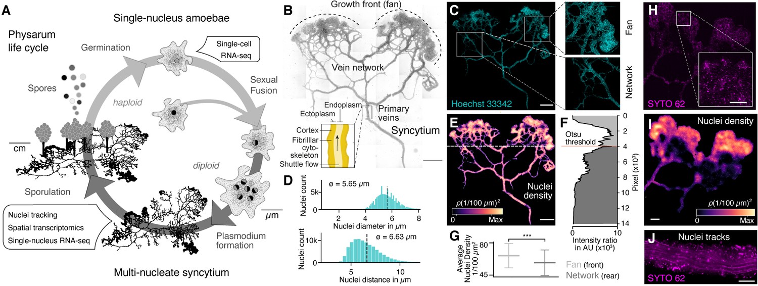
The slime mold Physarum polycephalum forms a multinucleate syncytium with mobile nuclei.
(A) Simplified life cycle of P. polycephalum indicating which experiments were performed in this study. (B) Plasmodium of P. polycephalum grows as a hierarchical network composed of contractile veins and a microstructured growth front. Tiled brightfield image of a fixed plasmodium is shown as reference. Scale bar: 1000 µm. (C) Hoechst-stained nuclei across the syncytium from (B) a growth front (top right) and a primary vein (bottom right). Scale bar: 1000 µm. (D) Histograms of nuclei diameter (top) and density (bottom) estimates are shown. Mean values are provided as insets. (E) Density map of nuclei after StarDist segmentation and kernel density estimation shows inhomogeneously distributed nuclei (see Materials and methods for further details). Scale bar: 1000 µm. (F) Averaged relative density estimates across the x-axis of the plasmodium are visualized along the y-axis of the plasmodium. A threshold by Otsu, 1979 was estimated to unbiasedly find a change in the density distribution separating the plasmodium in a network and a fan region. (G) Boxplots visualize the average nuclei density for the fan or network region identified in (F). p-value<0.001: *** (independent t-test, p=3.51 × 10⁻¹⁰). (H) Tiled life image of a plasmodium stained with SYTO 62 and a magnified fan region (inset). Scale bar: 500 µm. (I) Density map of nuclei shows that nuclei are not distributed homogeneously. Scale bar: 500 µm. (J) Maximum intensity projection over a period of 5 s of nuclei motion visualized by streamlines. See Video 1. Scale bar: 100 µm.
Figure 1—figure supplement 1
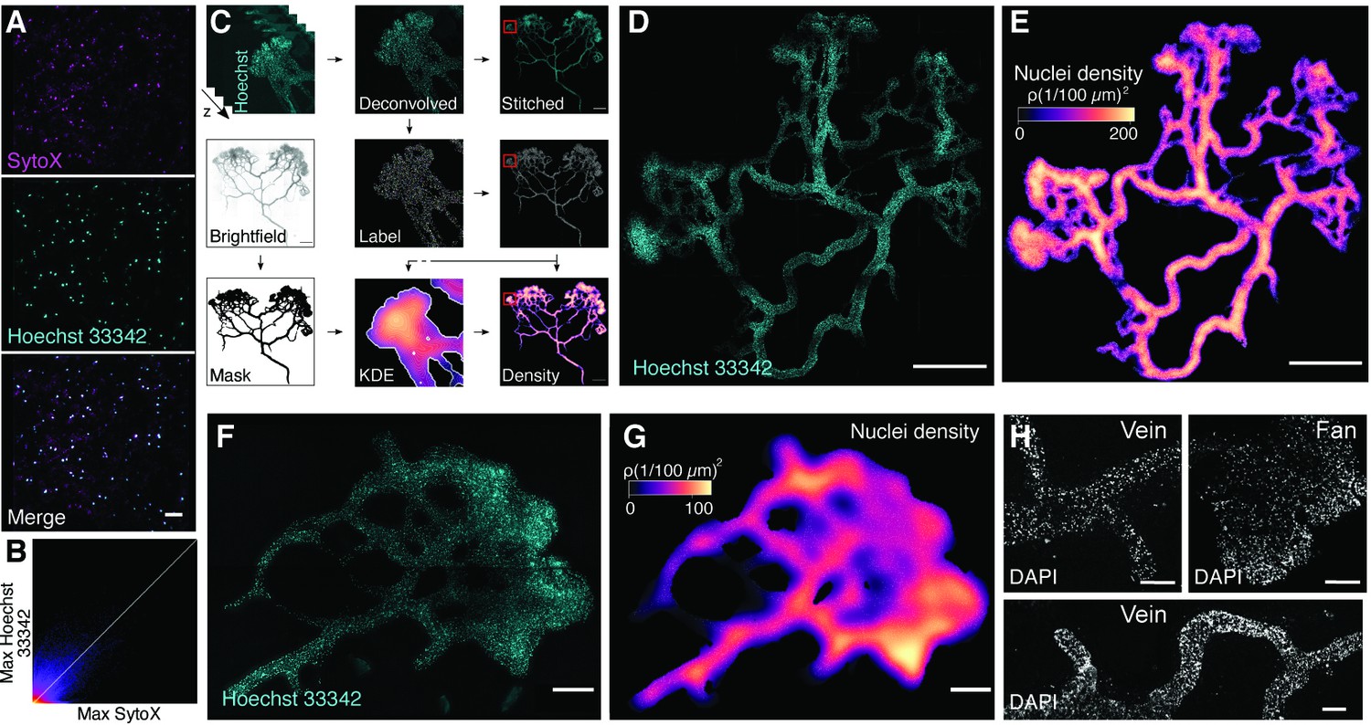
Nuclei are not homogeneously distributed across the multinucleate plasmodium.
(A) Colocalization tests of Hoechst and SYTO. Maximum projections are shown for SYTOX, Hoechst 33342, and the merged image (top to bottom). Scale bar: 50 µm. (B) Maximum 2D projection histogram revealing high correlation of SYTO and Hoechst (white line indicates Pearson’s R value 0.73). (C) Methodology workflow for imaging data analysis. Stitched: combining subimages to full-sized image; KDE, kernel density estimation. (D) Hoechst-stained nuclei across a fixed plasmodium. Scale bar: 1000 µm. (E) Density map of nuclei for the plasmodium shown in (B) after StarDist segmentation and kernel density estimation (Weigert et al., 2020). Scale bar: 1000 µm. (F) Hoechst-stained nuclei across a fixed plasmodium. Scale bar: 200 µm. (G) Density map of nuclei for the plasmodium shown in (F) after StarDist segmentation and kernel density estimation (Weigert et al., 2020). Scale bar: 200 µm. (H) DAPI-stained nuclei across a fixed plasmodium. Different regions of the plasmodium are shown. Scale bar: 500 µm.
Figure 2 with 3 supplements
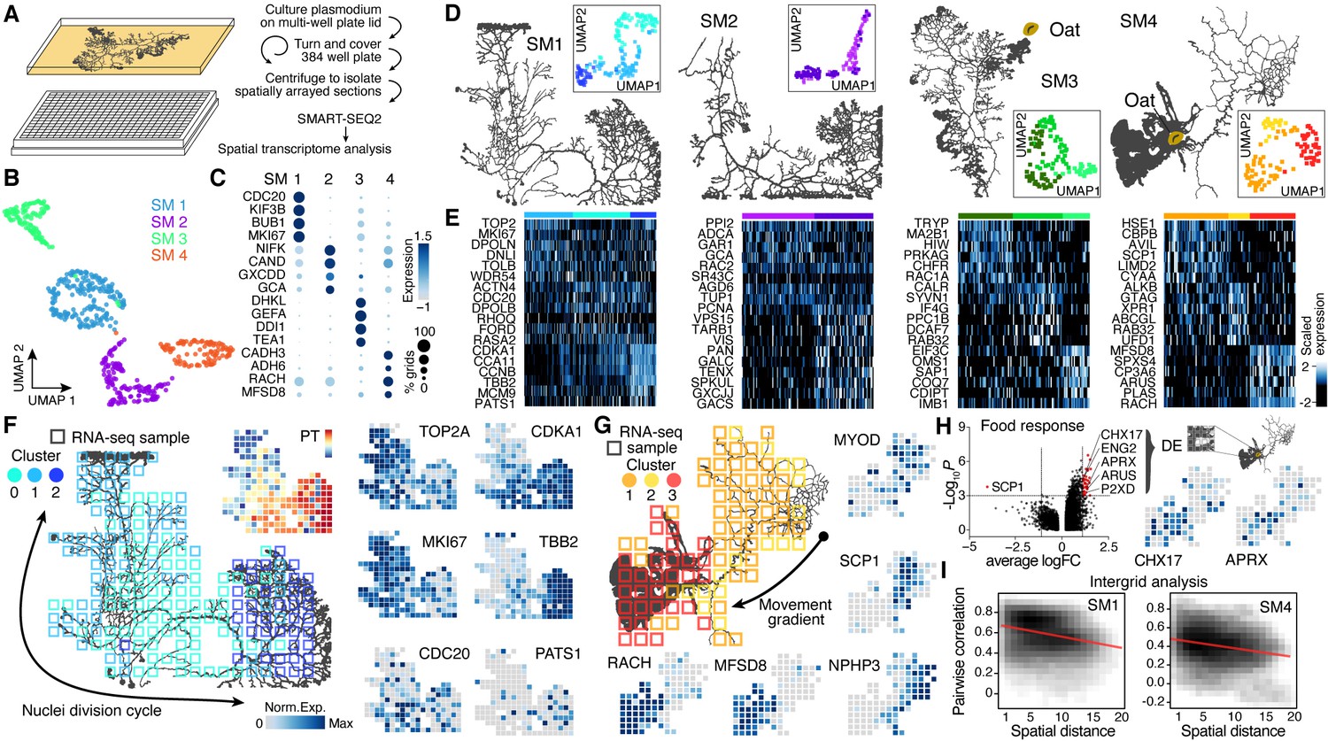
Spatial transcriptomics reveals region-specific gene expression in the plasmodial slime mold syncytia.
(A) Schematic of experimental setup. (B) Four slime mold plasmodia were grown overnight from a microplasmodia culture. Uniform Manifold Approximation and Projection (UMAP) embedding reveals general differences between slime molds. (C) Dotplot visualizes scaled gene expression intensity (dot color) and frequency (dot size) for top slime mold-specific marker genes, respectively. (D) Morphology overview of slime mold plasmodia investigated. SM1 and 2 were directly investigated after grown from microplasmodia culture, whereas oat flakes were supplied to SM3 and 4 and experiments were performed either just before the slime mold reached the food (SM3) or 4 hr after it reached the oat flake and had started re-expanding (SM4). UMAP embeddings next to each plasmodium reveal gene expression differences across grids for individual slime molds. (E) Heatmap representations of gene expression intensities for cluster markers (rows) across all grids (columns). Grids are ordered by cluster identity shown in (D). (F) Sampling grid on the 384-well plate overlaid by the plasmodium of SM1 at the time when sampled (left). Different colors represent the clustering result from (D). Right: marker genes from (E) are visualized as feature plots onto the sampling grid. (G) Sampling grid on the 384-well plate overlaid by the plasmodium of SM4 at the time when sampled (top left). Different colors represent the clustering result from (D). Bottom: marker genes from (E) are visualized as feature plots onto the sampling grid. (H) Volcano plot (left) reveals differentially expressed (DE) genes specific to grids where the plasmodium was in direct contact with a food source (oat flake). Feature plots (right) visualize the spatial arrangement for two of the DE genes of the volcano plot. (I) Density plots visualize the relation between the pairwise distance against the pairwise Pearson’s correlation across all samples of the grid of SM1 (left) and SM4 (right), respectively. Statistically significant negative correlations are identified and marked by a red line.
Figure 2—figure supplement 1

Spatial transcriptomics experiments allow to identify gene expression differences across plasmodial slime mold syncytia.
(A) Camera images showing four slime mold plasmodia just before spun into 384-well plates, respectively. Oat flakes had been removed for SM3 and 4. (B) Exemplary image of a 384-well plate after spinning SM1 into separate wells of the plate. (C) Principal components analysis (PCA) results for the combined RNA-seq dataset of all four slime molds. Each dot represents a single sample (well of the 384-well plate). (D) Feature plots show expression of exemplary genes that are shared between plasmodia. See Figure 2B for more information. (E) Uniform Manifold Approximation and Projection (UMAP) embedding of Harmony (Korsunsky et al., 2019) (left) and Seurat CCA (Stuart et al., 2019) (right) corrected data. (F) Louvain clusters identified for each embedding in (E), respectively, are shown (top) and are visualized for the respective other embedding (bottom) to compare the different corrected datasets. (G) Cluster-specific genes for Harmony-corrected data are shown as features on the UMAP embedding in Figure 2B. (H) UMAP embedding obtained by excluding unannotated transcripts (total: 15,120 transcripts) for all spatially resolved grids as shown in Figure 2B (top). The same grids were embedded by using all transcripts (total: 27,781 transcripts) (bottom). Different colors represent plasmodial origin. (I) Fan scores were calculated and are visualized as features on the grids of SM1−4. (J) Top 10 fan score grids of each plasmodium were extracted and unbiasedly embedded by UMAP. Hierarchical clustering results in two clusters (top) with SM3 being specific to cluster 2 (bottom). (K) Sampling grid on the 384-well plate overlaid by the plasmodium of SM2 at the time when sampled. Different colors represent the clustering result from Figure 2D. (L) Sampling grid on the 384-well plate overlaid by the plasmodium of SM3 at the time when sampled. Different colors represent the clustering result from Figure 2D. (M) Density plot visualizes the relation between the pairwise distance against the pairwise Pearson’s correlation across all grids of SM2. A statistically significant negative correlation is identified and marked by a red line. (N) Density plot visualizes the relation between the pairwise distance against the pairwise Pearson’s correlation across all grids of SM3. No clear correlation is identified as indicated by a red line.
Figure 2—figure supplement 2
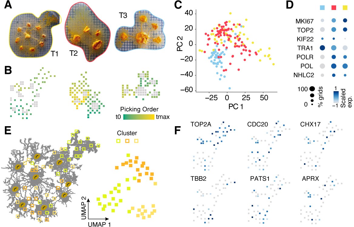
Spatial transcriptomics experiments with manual picking of plasmodial pieces.
(A) Camera images showing three slime mold plasmodia prior to consecutively picking individual pieces of roughly 2 × 2 mm into separate reaction tubes while keeping track of the picking location. Colored outlines are used to mark T1-3 on the following panels. (B) Sampling grids across the plasmodia in (A) with oat flakes visualized as gray squares to allow an optical overlay with the images in (A). The picking order is visualized as a feature onto the grids. (C) Principal components analysis (PCA) scatter plot of PC1 and 2 reveals separation of plasmodium T3 from the other two plasmodia. Same color legend as in (A) is depicted. (D) Dotplot representation of nuclei division genes that are identified to be top marker genes of plasmodium T1 and T2. Same color legend as in (A) is depicted. (E) Left: sampling grids are visualized as an overlay with the shape of plasmodium T1 and are colored by the clustering result. Right: Uniform Manifold Approximation and Projection (UMAP) embedding of sampling grids of T1. Colors depict cluster identity. (F) Gene expression is visualized as a feature on the UMAP embedding in (E). Early (TOP2A), medium (CDC20), and late (TBB2/PATS1) nuclei division cycle markers are shown. Coexpression of CHX17 and APRX is found in a region with high oat flake density.
Figure 2—figure supplement 3
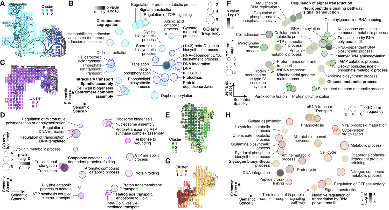
Gene Ontology (GO) analysis of cluster-specific genes across plasmodial slime mold syncytia.
(A) Cluster overview represented as a feature on the grids of SM1. (B) SM1 GO enrichments obtained by using GOseq on cluster-specific marker genes (Young et al., 2010) are visualized as dotplots using Revigo (Supek et al., 2011) with dot distances reflecting similarity of GO terms. Bold letters highlight SM1-specific terms. (C) Cluster overview represented as a feature on the grids of SM2. (D) Dotplot visualization of GO enrichments for SM2 as described in (B). (E) Cluster overview represented as a feature on the grids of SM3. Bold letters highlight SM3-specific terms. (F) Dotplot visualization of GO enrichments for SM3 as described in (B). (G) Cluster overview represented as a feature on the grids of SM4. Bold letters highlight SM4-specific terms. (H) Dotplot visualization of GO enrichments for SM4 as described in (B).
Figure 3 with 1 supplement
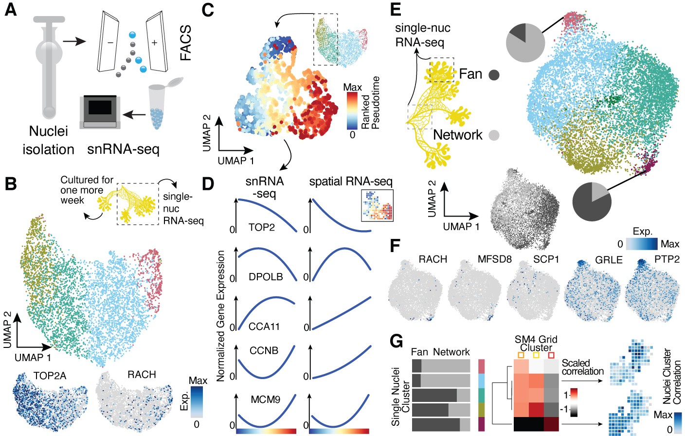
Single-nucleus RNA-sequencing uncovers nuclei diversification within the syncytia.
(A) Nuclei extraction using a douncer with subsequent nuclei enrichment through FACS was performed prior to single-nucleus experiments. (B) Uniform Manifold Approximation and Projection (UMAP) embedding visualizes nuclei heterogeneity of a freshly grown plasmodium. Cluster-specific marker genes are visualized as features on the embedding. (C) Pseudotemporal ordering of nuclei extracted from clusters with high TOP2A expression in (B). Extracted nuclei were re-embedded by UMAP with pseudotime ranks shown on the embedding. (D) Gene expression changes of cluster marker (see Figure 2F) genes across pseudotime are shown for snRNA-seq (left) and spatially resolved grid RNA-seq data (right). (E) UMAP embedding reveals nuclei heterogeneity of a 1-week-old slime mold plasmodium with nuclei originating from different parts of the plasmodium. Pie charts reveal different nuclei proportions of two exemplary clusters. The UMAP inset encodes the origin of each nucleus by color. (F) Cluster marker genes for (E) are presented as feature plots on the embedding. (G) From left to right: bar chart representing proportions of nuclei origin per cluster shown in (E). Heatmap representation of scaled correlation values between the pseudobulk gene expression per cluster of the plasmodium in (E) and the pseudobulk gene expression per cluster for SM4 (Figure 2G). Arrows indicate for which clusters correlations against individual grids of SM4 were estimated with the result being presented as a feature on the grid embedding.
Figure 3—figure supplement 1
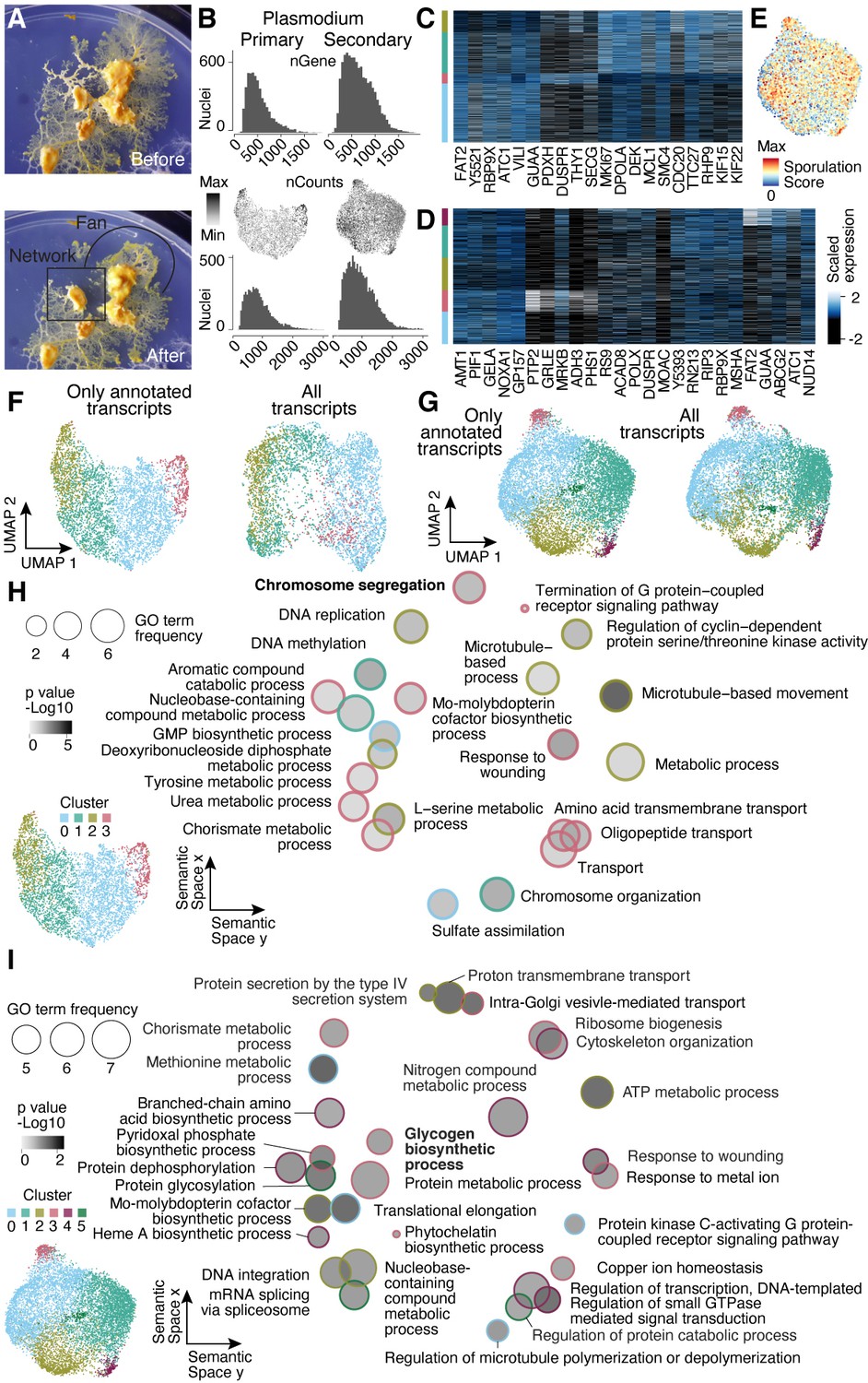
Nuclei heterogeneity revealed by single-nuclei RNA-seq.
(A) Camera images show the secondary plasmodium before and after sampling a fan- and network-enriched sample (encircled by black lines), respectively, for the snRNA-seq experiment. (B) Histograms visualize transcript (bottom) and gene (top) detection counts per nucleus for each plasmodium sampled. Center: feature plots show transcript detection counts on Uniform Manifold Approximation and Projection (UMAP) embedding. (C) Heatmap representation of marker gene expression for primary plasmodium clusters shown in Figure 4B. (D) Heatmap representation of marker gene expression for secondary plasmodium clusters shown in Figure 4E. (E) Sporulation score is shown as a feature onto the UMAP embedding in Figure 4E. The score was estimated as the sum of transcript counts for a list of fruiting body formation specific genes (Glöckner and Marwan, 2017). (F) UMAP embedding and clusters (indicated by different colors) obtained by excluding unannotated transcripts (total: 14,055 transcripts) for the primary plasmodium as shown in Figure 3B (left). The same nuclei were embedded by using all transcripts (total: 24,592 transcripts) with different colors representing the clusters in Figure 3B (right). (G) UMAP embedding and clusters (indicated by different colors) obtained by excluding unannotated transcripts (total: 14,483) for the secondary plasmodium (see Figure 3E) (left). The same nuclei were embedded by using all transcripts (total: 25,815) with different colors representing the clusters in Figure 3E (right). (H) Primary plasmodium-specific Gene Ontology (GO) enrichments (right) obtained by using GOseq on cluster-specific marker genes (see Figure 3B and inset bottom left; Young et al., 2010) are visualized as dotplots using Revigo (Supek et al., 2011) with dot distances reflecting similarity of GO terms. Bold letters highlight shared terms between primary plasmodium and SM1. (I) Dotplot visualization of GO enrichments for the secondary plasmodium as described in (B) (right). Bold letters highlight shared terms between the secondary plasmodium and SM4. See Figure 3E and inset (bottom left) for more cluster information.
Figure 4 with 1 supplement
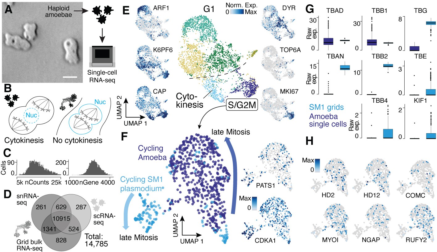
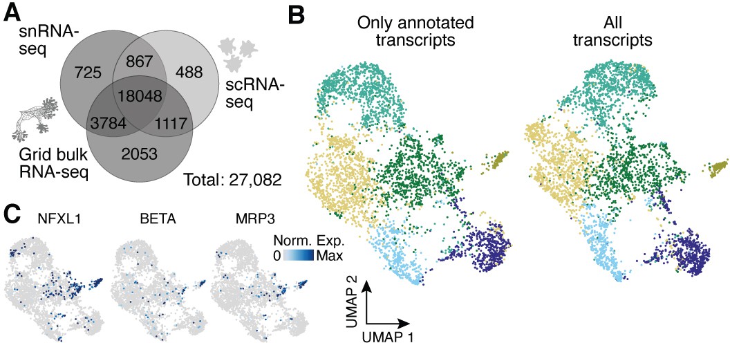
Single-nucleus amoebae are heterogeneous and differentially regulate cytokinetic programs compared with syncytial nuclei.
(A) Brightfield image of amoebae (single frame from Video 3). Scale bar: 10 µm. (B) Schematic illustrating mechanistic differences during mitosis in amoebae (left) and plasmodia (right). (C) Histograms reveal the distribution of the raw transcript counts per gene (left) and the number of different genes per cell detected (right) for amoeba scRNA-seq data. (D) Venn diagram shows the number of genes detected per experimental setup and their overlap. A 10% quantile cutoff was applied to remove sparsely expressed genes for the comparison. (E) Uniform Manifold Approximation and Projection (UMAP) embedding of single haploid amoeba cells (center). Cell cycle stages are indicated and gene expression intensities are visualized as features on the embedding (left/right). (F) UMAP embedding of single amoeba cells in G2M phase and samples of a cycling plasmodium (SM1). RNA-seq samples were integrated using Seurat’s built-in CCA ‘anchoring’ (Stuart et al., 2019) to allow a comparison between single-cell (10x Genomics) and bulk RNA-seq (SmartSeq2) data. Feature plots of PATS1 and CDKA1 reveal cell/nuclei cycle directionality for samples. Drawn arrows reveal directionality. (G) Cell cycle-related marker gene expression identified through cluster-specific gene expression analysis between amoeba cells and plasmodium grids in (F) is visualized as a boxplot for plasmodium and amoeba samples, respectively. TBAD and TBB1 are shown as reference for non-DE genes. (H) Amoeba-specific genes are visualized as feature plots on the UMAP embedding in (F).
Figure 4—figure supplement 1
Analysis of the impact of unannotated transcripts on amoeba cell heterogeneity.
(A) Venn diagram shows the number of genes detected per experimental setup and their overlap when using all transcripts of the transcriptome as compared to using only annotated transcripts in Figure 4D. A 10% quantile cutoff was applied to remove sparsely expressed genes for the comparison. (B) Uniform Manifold Approximation and Projection (UMAP) embedding and clusters (indicated by different colors) obtained by excluding unannotated transcripts (total: 13,802 transcripts) for single amoeba transcriptomes as shown in Figure 4E (left). The same cells were embedded by using all transcripts (total: 22,905 transcripts) with colors representing the clusters in Figure 4E (right). (C) Feature plots highlight additional cluster-specific marker genes for amoeba cluster 5.
Author response image 1
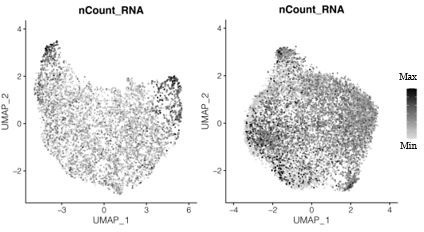
Transcript counts per nucleus for snRNA-seq data for the primary plasmodium (left) and the secondary plasmodium (right).
Videos
Video 1
Nuclei shuttle flow in a primary vein of a network region.
Live recording of SYTO62-stained nuclei in a primary vein of a network region of a Physarum plasmodium. Nuclei shuttle within the cytoplasmic flow. While some nuclei get trapped in the ectoplasm, others are released from the ectoplasm into the cytoplasmic flow. Differences in nuclei sizes originate from the single imaging plane of the three-dimensional tubes of the plasmodium and rarely by contamination of the autofluorescence of larger vesicles.
Video 2
Nuclei shuttle flow across a fan region.
Live recording of SYTO62-stained nuclei in a fan region of a Physarum plasmodium over one period of cytoplasmic shuttle streaming. Differences in nuclei sizes originate from the single imaging plane of the three-dimensional tubes of the plasmodium and rarely by contamination of the autofluorescence of larger vesicles.
Video 3
Living amoeba.
Brightfield live recording of haploid single-nucleus Physarum amoebae.
Additional files
-
Supplementary file 1
Sample overview.
- https://cdn.elifesciences.org/articles/69745/elife-69745-supp1-v1.xlsx
-
Supplementary file 2
Metadata for spatial transcriptomics dataset SM1.
Excel sheets containing sampling information, sequencing library pooling scheme, and metadata such as grid coordinates and sequencing depth per grid. Sequencing depth is provided as the number of paired reads per grid, and only the grids that are analyzed in the article are listed on sheet 3.
- https://cdn.elifesciences.org/articles/69745/elife-69745-supp2-v1.xlsx
-
Supplementary file 3
Metadata for spatial transcriptomics dataset SM2.
Excel sheets containing sampling information, sequencing library pooling scheme, and metadata such as grid coordinates and sequencing depth per grid. Sequencing depth is provided as the number of paired reads per grid, and only the grids that are analyzed in the article are listed on sheet 3.
- https://cdn.elifesciences.org/articles/69745/elife-69745-supp3-v1.xlsx
-
Supplementary file 4
Metadata for spatial transcriptomics dataset SM3.
Excel sheets containing sampling information, sequencing library pooling scheme, and metadata such as grid coordinates and sequencing depth per grid. Sequencing depth is provided as the number of paired reads per grid, and only the grids that are analyzed in the article are listed on sheet 3.
- https://cdn.elifesciences.org/articles/69745/elife-69745-supp4-v1.xlsx
-
Supplementary file 5
Metadata for spatial transcriptomics dataset SM4.
Excel sheets containing sampling information, sequencing library pooling scheme, and metadata such as grid coordinates and sequencing depth per grid. Sequencing depth is provided as the number of paired reads per grid, and only the grids that are analyzed in the article are listed on sheet 3.
- https://cdn.elifesciences.org/articles/69745/elife-69745-supp5-v1.xlsx
-
Supplementary file 6
Metadata for spatial transcriptomics dataset T1–3.
Excel sheets containing sampling information, sequencing library pooling scheme, and metadata such as grid coordinates and sequencing depth per grid. Sequencing depth is provided as the number of total reads per grid.
- https://cdn.elifesciences.org/articles/69745/elife-69745-supp6-v1.xlsx
-
Supplementary file 7
Cluster marker and Gene Ontology (GO) term enrichments.
Excel sheets containing cluster marker information and GOseq enrichments to explore the complete list of gene expression differences identified. Lists presented are sorted by the corresponding figure numbers.
- https://cdn.elifesciences.org/articles/69745/elife-69745-supp7-v1.xlsx
-
Transparent reporting form
- https://cdn.elifesciences.org/articles/69745/elife-69745-transrepform1-v1.docx
Download links
A two-part list of links to download the article, or parts of the article, in various formats.
Downloads (link to download the article as PDF)
Open citations (links to open the citations from this article in various online reference manager services)
Cite this article (links to download the citations from this article in formats compatible with various reference manager tools)
Spatial transcriptomic and single-nucleus analysis reveals heterogeneity in a gigantic single-celled syncytium
eLife 11:e69745.
https://doi.org/10.7554/eLife.69745


