Quantifying chromosomal instability from intratumoral karyotype diversity using agent-based modeling and Bayesian inference
- Carbone Cancer Center, University of Wisconsin-Madison, United States
- McArdle Laboratory for Cancer Research, University of Wisconsin-Madison, United States
- Department of Cell and Regenerative Biology, University of Wisconsin, United States
- Division of Hematology Medical Oncology and Palliative Care, Department of Medicine University of Wisconsin, United States
Figures
Figure 1 with 2 supplements
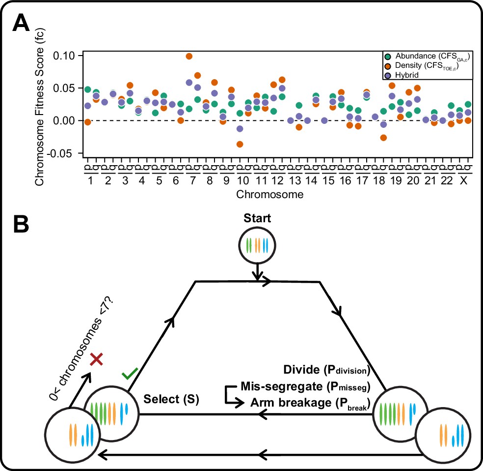
A framework for modeling CIN and karyotype selection.
(A) Chromosome arm scores for each model of karyotype selection. Gene Abundance scores are derived from the number of genes per chromosome arm normalized to the number of all genes. Chromosome arms 13 p and 15 p did not have an abundance score and were set to 0. Driver Density scores come from the pan-cancer chromosome arm scores derived in Davoli et al., 2013, and normalized to the sum of chromosome arm scores for chromosomes 1-22,X. Chromosome arms 13 p, 14 p, 15 p, 21 p, 22 p, and chromosome X did not have driver scores and were set to 0. Hybrid model scores are set to the average of the Driver and Abundance models. The neutral model (not displayed) is performed with all cell’s fitness constitutively equal to 1 regardless of karyotype. (B) Framework for the simulation of and selection on cellular populations with CIN. Cells divide (Pdivision starts at 0.5 in the exponential pseudo-Moran model and is constitutively equal to 1 for the constant Wright-Fisher model) and probabilistically mis-segregate chromosomes (Pmisseg ∈ [0, 0.001… 0.05]). After, cells experience selection under one of the selection models, altering cellular fitness and the probability (Pdivision) a cell will divide again (green check). Additionally, cells wherein the copy number of any chromosome falls to zero or surpasses 6 are removed (red x). After this, the cycle repeats. See Materials and methods for further details.
Figure 1—figure supplement 1
Expanded model of chromosome mis-segregation and karyotypic selection.
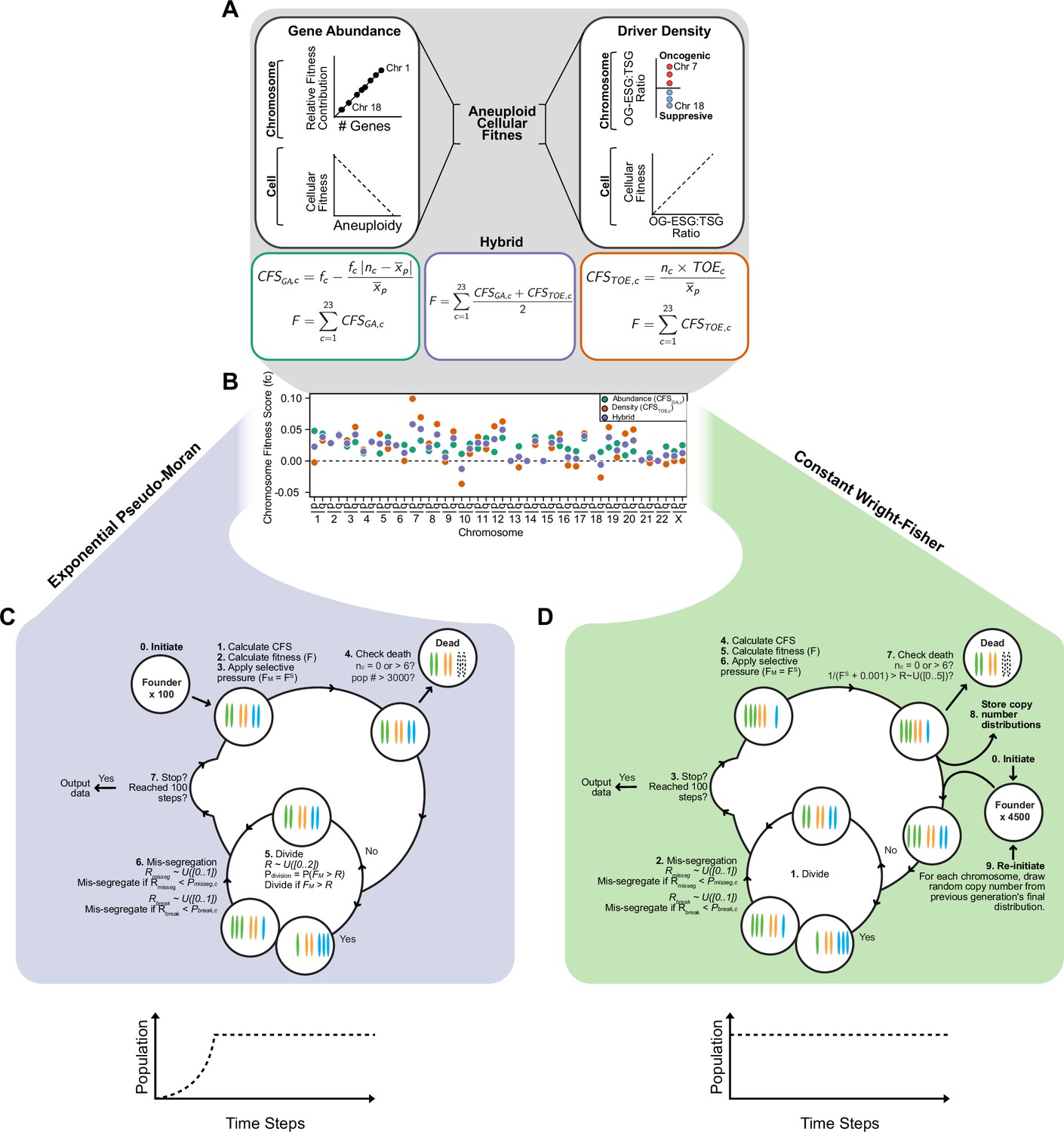
Models of selection on aneuploid karyotypes. Left. In the Gene Abundance model, chromosomes that encode a larger number of genes contribute more to cellular fitness (F). Thus, large chromosomes have a higher fitness score (fc). Deviation from the average ploidy of the population results in a reduced Contextual Fitness Score (CFS) for each chromosome, the sum of which represents the fitness of the cell. Right. In the Driver Density Model, the fitness contribution of a chromosome depends on the ratio of oncogenes and essential genes to tumor suppressors (OG-ESG:TSG). Gaining chromosomes with a higher OG-ESG:TSG ratio provides a fitness advantage while gaining more suppressive chromosomes invokes a fitness cost. These scores are still normalized to the ploidy of the average ploidy of the population to ensure that higher ploidy populations are not arbitrarily more fit. Middle. The Hybrid model takes the average of the fitness scores calculated in the other models. The neutral selection model (not shown) treats all karyotypes as equally fit. Base chromosome arm fitness scores for each model. Only the Hybrid and Driver Density model have negatively scored chromosomes, meaning their loss provides a fitness benefit. The neutral selection model does not require chromosome arm fitness scores. Simulating CIN in exponentially growing populations with pseudo-Moran limits. (0) Populations are founded by 100 founder cells and the simulation is initiated. (1) CFS values are calculated for each chromosome in a cell according to the chosen model. (2) Cellular fitness is calculated based on CFS values. (3) Selective pressure (S) is applied on cellular fitness values (F). (4) Cells are checked to see if any death conditions are met and if the population limit is met. (5) Cells probabilistically enter mitosis if their fitness value exceeds a random float (R) between 0 and 2. Thus Pdivision = P(FM >R). If a cell does not divide, it skips the next step. (6) If a cell enters mitosis, each chromosome has an opportunity to mis-segregate probabilistically. For each chromosome, a mis-segregation occurs if a random float (R), from 0 to 1, falls below Pmisseg. After a chromosome mis-segregation is determined, the chromosome arms may be individually segregated (i.e. reciprocal CNA) if a random float (R), from 0 to 1, falls below Pbreak. The cycle repeats and new CFS values are calculated, unless (7) stop conditions are met. When populations reach or exceed 3500 cells, a random half of the population is eliminated and the remaining cells continue the cycle. Simulating CIN in constant-size populations with Wright-Fisher dynamics. (0) Populations are initiated by 4500 euploid cells which (1) divide every step. (2) Chromosomes are mis-segregated as in the exponential pseudo-Moran model described above. (3) If stop conditions are met, the simulation ends and data are exported. If the cycle continues, (4) CFS values are calculated and used to (5) determine cellular fitness, after which, (6) selective pressure is applied. (7) Cells die if they lose both copies of a chromosome or exceed the upper limit of six. Additionally, to approximate Wright-Fisher dynamics, cells die if 1/(FS +0.001) exceeds a random float from 0 to 5. Thus, the baseline rate of cell death is ~0.2. (8) Each chromosome copy number is stored and the population is re-initiated with 4500 new cells. The copy numbers for each of new cell’s chromosomes are randomly and independently drawn from the copy number distributions of the previous generation. The cycle then repeats until the simulation ends (step 3).
Figure 1—figure supplement 2
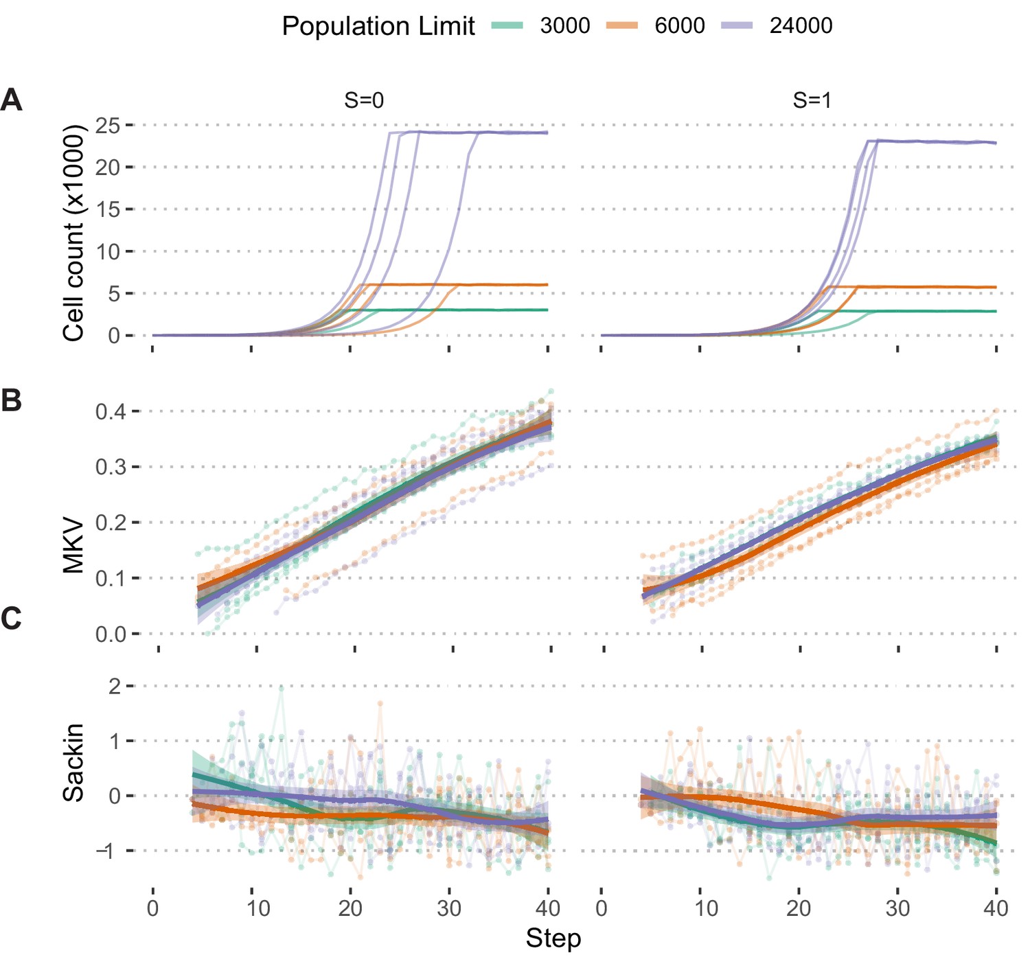
Population growth limits do not bias population measures.
(A) Growth curves of populations simulated under the Hybrid selection model and exponential pseudo-Moran growth model with S ∈[0,1] and Pmisseg misseg = 0.022 and limited to 3000, 6000, and 24,000 cells (n = 4 simulations each). (B) MKV (normalized to mean ploidy of the population) values steadily increase over time. (C) Loess regression curves show no significant deviations based on the population threshold, regardless of selection. Tree-tip-normalized Sackin index values for each population over time. No significant deviations based on the population threshold, regardless of selection.
Figure 2 with 2 supplements
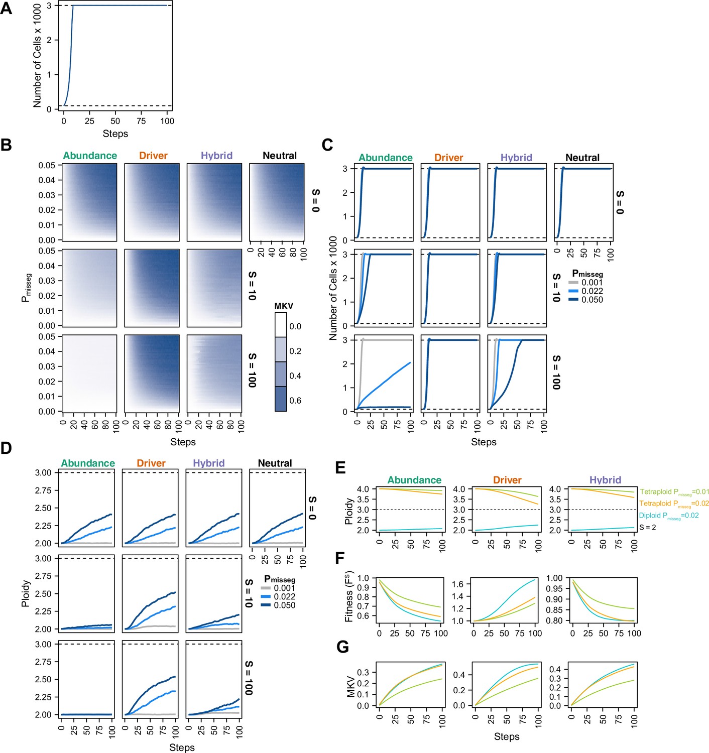
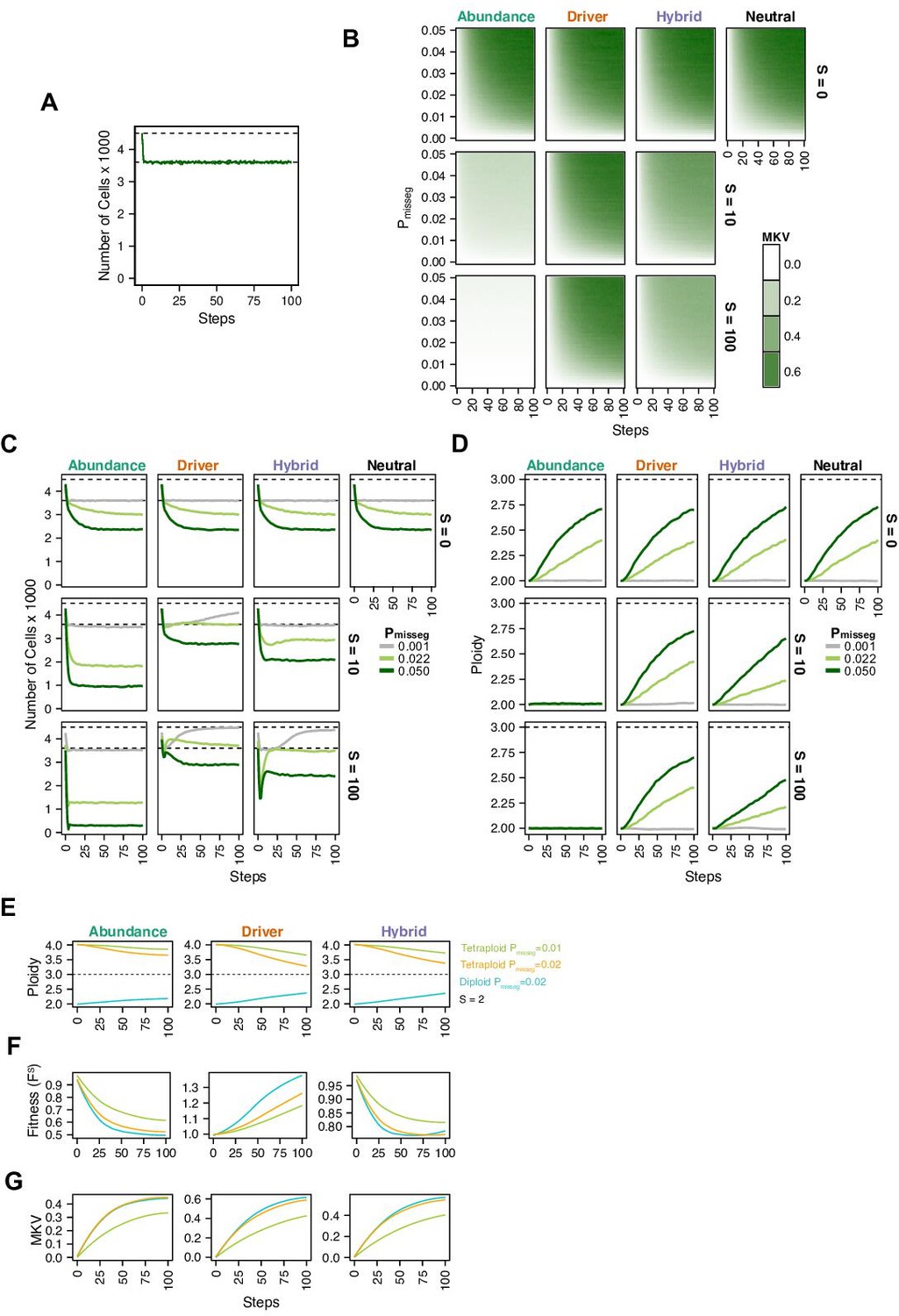
Evolutionary dynamics imparted by CIN.
(A) Population growth curve in the absence of selective pressure (Pmisseg = 0.001, S = 0, n = 3 simulations). The steady state population in null selection conditions is 3000 cells. (B) Heatmaps depicting dynamics of karyotype diversity as a function of time (steps), mis-segregation rate (Pmisseg), and selection (S) under each model of selection. Columns represent the same model; rows represent the same selection level. Mean karyotype diversity (MKV) is measured as the variance of each chromosome averaged across all chromosomes 1–22, and chromosome X. Low and high MKV are shown in white and blue respectively (n = 3 simulations for every combination of parameters). (C) Population growth under each model, varying Pmisseg and S. Pmisseg∈ [0.001, 0.022, 0.050] translate to about 0.046, 1, and 2.3 mis-segregations per division respectively for diploid cells. (D) Dynamics of the average ploidy (total # chromosome arms / 46) of a population while varying Pmisseg and S. (E) Dynamics of ploidy under each model for diploid and tetraploid founding populations. Pmisseg∈ [0.01, 0.02] translate to about 0.46 and 0.92 mis-segregations for diploid cells and 0.92 and 1.84 mis-segregations for tetraploid cells. (F) Fitness (FS) over time for diploid and tetraploid founding populations evolved under each model. (G) Karyotype diversity dynamics for diploid and tetraploid founding populations. MKV is normalized to the mean ploidy of the population at each time step. Plotted lines in C-G are local regressions of n = 3 simulations.
Figure 2—figure supplement 1
Chromosomal instability and karyotype selection in constant-size populations approximating Wright-Fisher dynamics.
(A) Population size over time in the absence of selective pressure (Pmisseg = 0.001, S = 0, n = 3 simulations). The steady state population in null selection conditions is ~3600 cells as data is exported before populations are re-initiated. Dashed line represents the population at (re-)initiation (4500 cells). (B) Heatmaps depicting dynamics of karyotype diversity as a function of time (steps), mis-segregation rate (Pmisseg), and selection (S) under each model of selection. Columns represent the same model; rows represent the same selection level. Mean karyotype diversity (MKV) is measured as the variance of each chromosome averaged across all chromosomes 1–22, and chromosome X. Low and high MKV are shown in white and green respectively (n = 3 simulations for every combination of parameters). (C) Population growth under each model, varying Pmisseg and S. Pmisseg∈ [0.001, 0.022, 0.050] translate to about 0.046, 1, and 2.3 mis-segregations per division respectively for diploid cells. Top dashed line represents the population at (re-)initiation (4500 cells). Bottom dashed line represents the steady state population in selection-null conditions. (D) Dynamics of the average ploidy (total # chromosome arms / 46) of a population while varying Pmisseg and S. (E) Dynamics of ploidy under each model for diploid and tetraploid founding populations. Pmisseg∈ [0.01, 0.02] translate to about 0.46 and 0.92 mis-segregations for diploid cells and 0.92 and 1.84 mis-segregations for tetraploid cells. (F) Fitness (FS) over time for diploid and tetraploid founding populations evolved under each model. (G) Karyotype diversity dynamics for diploid and tetraploid founding populations. MKV is normalized to the mean ploidy of the population at each time step. Plotted lines in C-G are local regressions of n = 3 simulations.
Figure 2—figure supplement 2
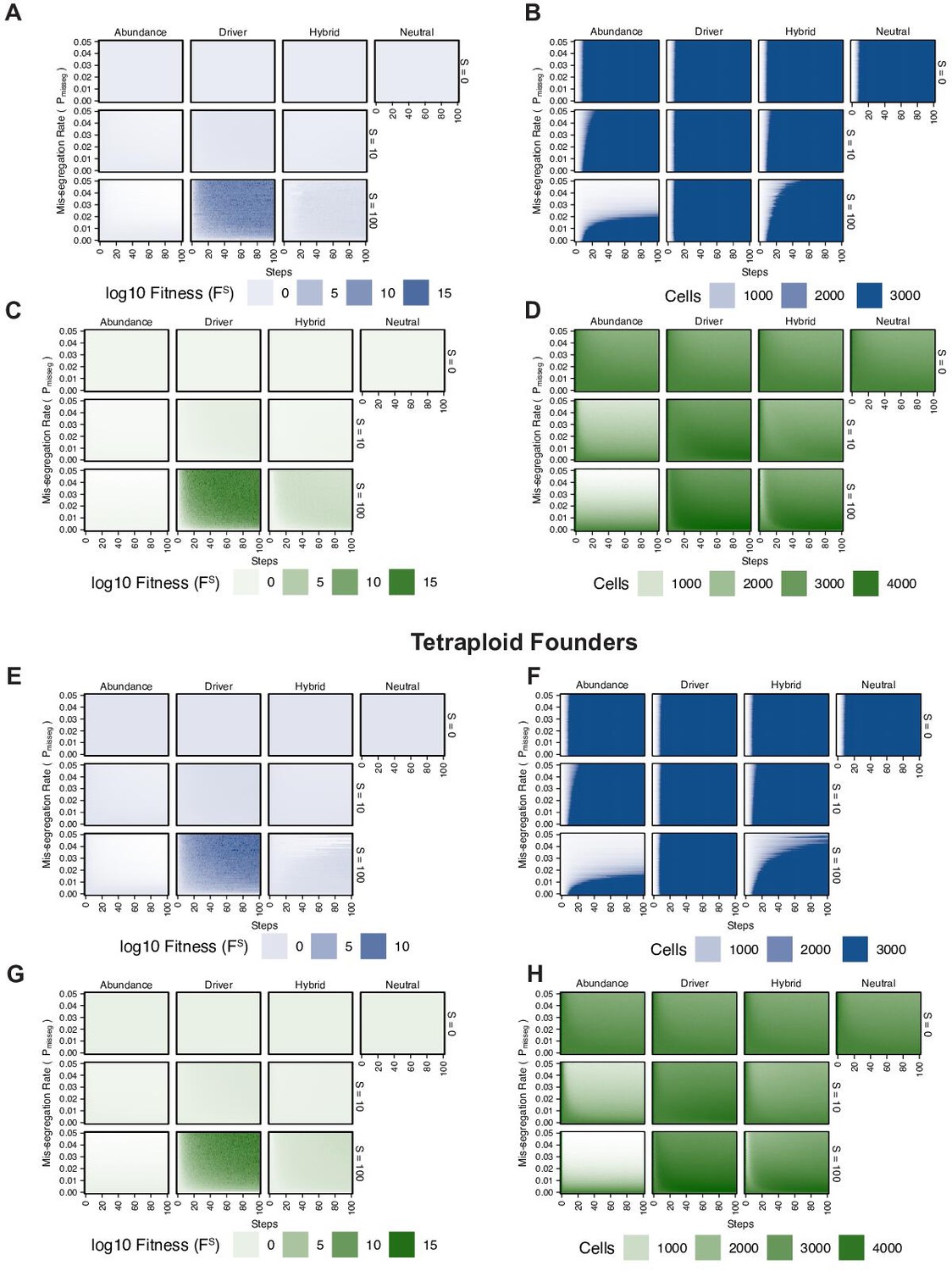
Fitness of diploid and tetraploid CIN +populations.
(A) Fitness landscape of simulations founded by diploid cells under exponential pseudo-Moran growth dynamics. (B) Size of simulated populations founded by diploid cells under exponential pseudo-Moran growth dynamics. (C) Fitness landscape of simulations founded by diploid cells under constant Wright-Fisher growth dynamics. (D) Size of simulated populations founded by diploid cells under constant Wright-Fisher growth dynamics. (E) Fitness landscape of simulations founded by tetraploid cells under exponential pseudo-Moran growth dynamics. (F) Size of simulated populations founded by tetraploid cells under exponential pseudo-Moran growth dynamics. (G) Fitness landscape of simulations founded by tetraploid cells under constant Wright-Fisher growth dynamics. (H) Size of simulated populations founded by tetraploid cells under constant Wright-Fisher growth dynamics.
Figure 3 with 1 supplement

Karyotype diversity depends profoundly on selection modality.
(A) Simulation scheme to assess long-term dynamics of karyotype evolution and karyotype convergence. (B) Heatmaps depicting the chromosome copy number profiles of a subset (n = 30 out of 300 sampled cells) of the simulated population with early CIN over time under each model of karyotype selection. (C) Average heatmaps (lower) show the average copy number across the 5 replicates for (1) the Exponential Psuedo-Moran (Base), (2) the base model with the upper copy number limit set to 10, (3) the base model that invokes a FM x 0.1 penalty for any cell with a haploid chromosome, (4) and the Constant Population-Size Wright-Fisher model. Pmisseg = 0.003; S = 25 (except Neutral model; S = 0); ploidy = 2.
Figure 3—figure supplement 1
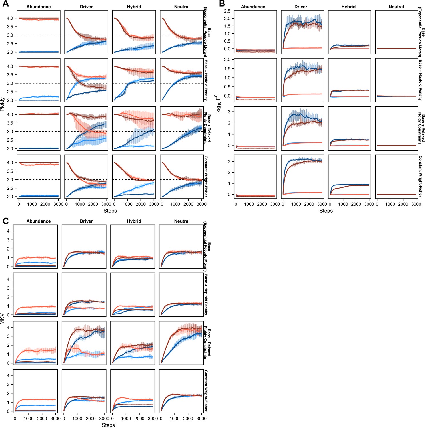
Modeled population measures tracked over time.
(A) Average population ploidy over time for each selection model within each model variation. Data represent the mean and range (vertical lines) across five replicates for every 50 time steps in diploid populations with low selective pressure (light red) and high selective pressure (dark red) and tetraploid populations with low selective pressure (light blue) and high selective pressure (dark blue). (B) Average population fitness (log10) over time for each selection model within each model variation. Data represent the mean and range (vertical lines) across five replicates for every 50 time steps in diploid populations with low selective pressure (light red) and high selective pressure (dark red) and tetraploid populations with low selective pressure (light blue) and high selective pressure (dark blue). (C) Mean karyotype variance over time for each selection model within each model variation. Data represent the mean and range (vertical lines) across five replicates for every 50 time steps in diploid populations with low selective pressure (light red) and high selective pressure (dark red) and tetraploid populations with low selective pressure (light blue) and high selective pressure (dark blue).
Figure 4

Topological features of simulated phylogenies delineate CIN rate and karyotype selection.
(A) Quantifiable features of karyotypically diverse populations. Heterogeneity between and within karyotypes is described by MKV and aneuploidy (inter- and intra-karyotype variance, see Materials and methods). We also quantify discrete topological features of phylogenetic trees, such as cherries (tip pairs) and pitchforks (3-tip groups), and a whole-tree measure of imbalance (or asymmetry), the Colless index. (B) Scheme to test how CIN and selection influence the phylogenetic topology of simulated populations. (C) Computed heterogeneity (aneuploidy and MKV) and topology (Colless index, cherries, pitchforks) summary statistics under varying Pmisseg and S values. MKV is normalized to the average ploidy of the population. Topological measures are normalized to population size. Spearman rank correlation coefficients (r) and p-values are displayed (n = 8 simulations). (D) Representative phylogenies for each hi/low CIN, hi/low selection parameter combination and their computed summary statistics. Each phylogeny represents n = 50 out of 300 cells for each simulation. (E) Dimensionality reduction of all simulations for each hi/low CIN, hi/low selection parameter combination using measures of karyotype heterogeneity only (left; MKV and aneuploidy) or measures of karyotype heterogeneity and phylogenetic topology (right; MKV, aneuploidy, Colless index, cherries, and pitchforks).
Figure 5 with 5 supplements
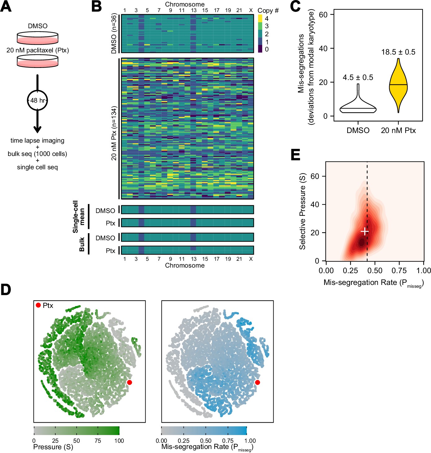
Experimental chromosome mis-segregation measured by Bayesian inference experimental scheme.
(A) Cal51 cells were treated with either DMSO or 20 nM paclitaxel for 48 hr prior to further analysis by time lapse imaging, bulk DNA sequencing, and scDNAseq. (B) Heatmaps showing copy number profiles derived from scDNAseq data, single-cell copy number averages, and bulk DNA sequencing. (C) Observed mis-segregations calculated as the absolute sum of deviations from the observed modal karyotype of the control. (D) Dimensionality reduction analysis of population summary statistics (aneuploidy, MKV, Colless index, cherries) from the first three time steps of all simulations performed under the Hybrid model. (E) 2D density plot showing joint posterior distributions from ABC analysis using population summary statistics computed from the paclitaxel-treated cells using the following priors and parameters: Growth Model = ‘exponential pseudo-Moran’, Selection Model = ‘Hybrid, initial ploidy = 2, 2 time steps, S ∈[0, 2… 100], Pmisseg∈[0, 0.005… 1.00] and a tolerance threshold of 0.05 to reject dissimilar simulation results. (see Materials and Methods). Vertical dashed line represents the experimentally observed mis-segregation rate. White + represents the mean of inferred values.
Figure 5—figure supplement 1
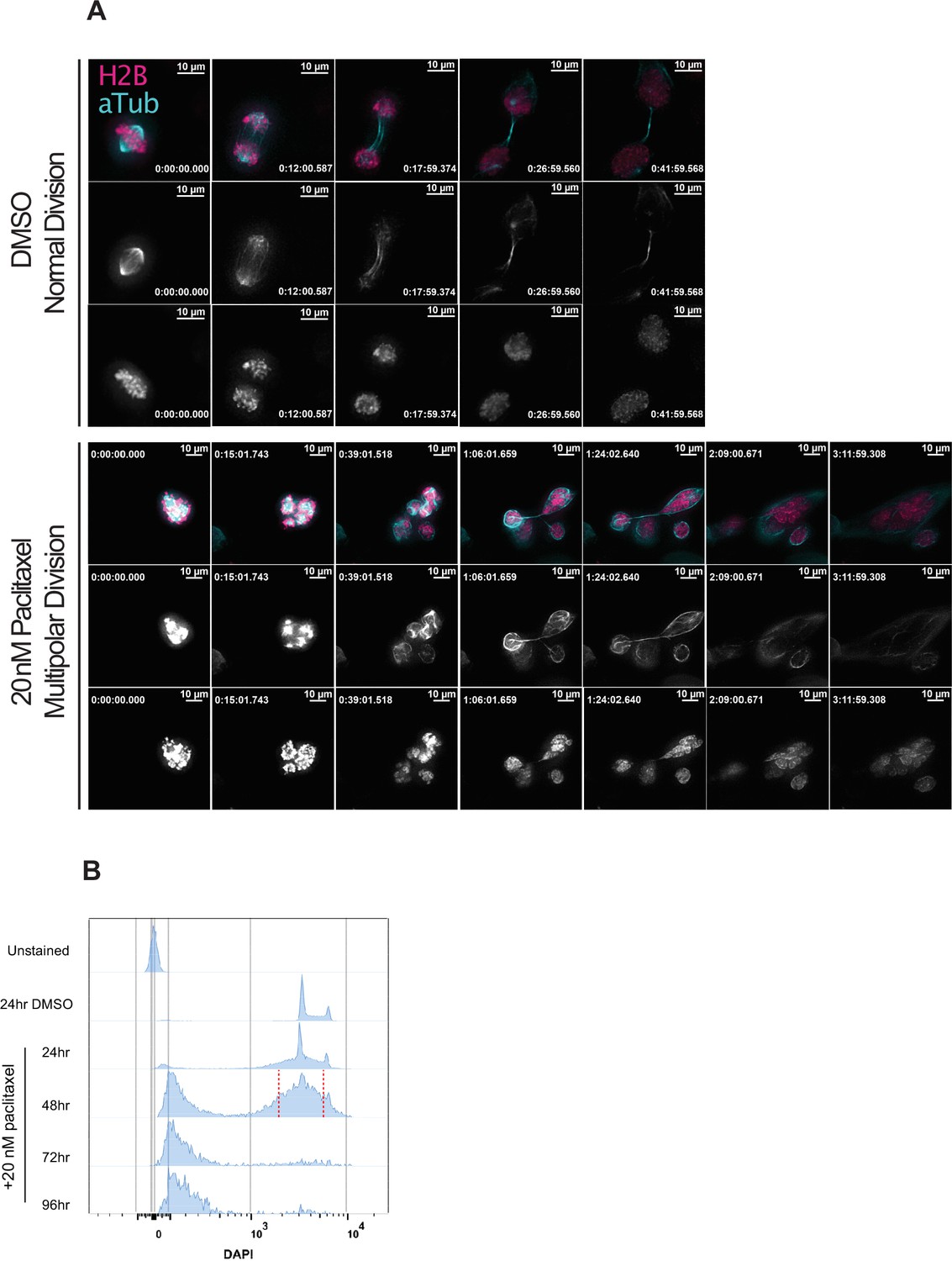
Induction of extensive chromosome mis-segregation via paclitaxel.
(A) Immunofluorescence time lapse montage of control Cal51 cells undergoing normal mitosis (top) and paclitaxel-treated treated cells undergoing a multipolar anaphase (middle) and partial cytokinesis failure (bottom). (B) Cell cycle profiles from flow cytometric analysis of Cal51 cells treated with either DMSO (72 hr) or 20 nM paclitaxel for 24, 48, or 72 hr. For FACS, cells treated for 48 hr were sorted into individual wells of 96-well plates. Sorting gate is shown by the red, dashed line.
Figure 5—figure supplement 2
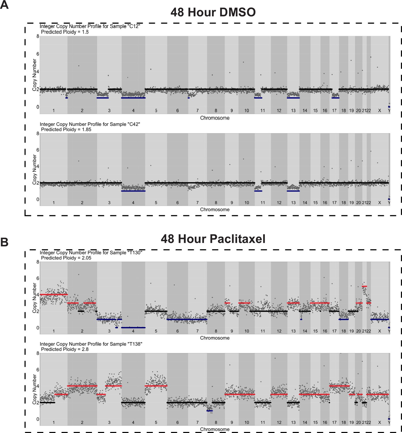
Copy number profiles of DMSO- and paclitaxel-treated Cal51 cells.
Single-cell copy number profiles for single (A) DMSO- and (B) paclitaxel-treated cells. A total of 500 Kb genomic bins and DNA content from FACS were used for copy number calculations (see Materials and methods).
Figure 5—figure supplement 3
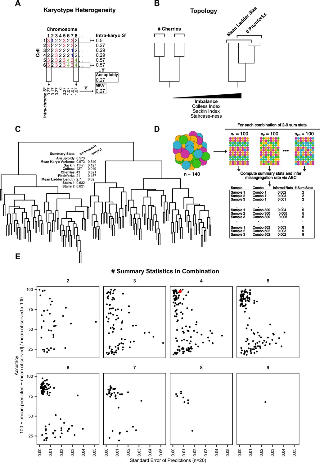
Summary statistic optimization for ABC.
(A) Schematic showing calculation of aneuploidy and MKV. (B) Examples of phylogenetic topology metrics. (C) Phylogenetic reconstruction of a population of Cal51 cells treated with 20 nM paclitaxel for 48 hr and associated heterogeneity and topology metrics. Normalized and non-normalized summary statistics are displayed (see Materials and methods). (D) Analytical scheme to identify most accurate and least variable combinations of heterogeneity and topology metrics. For each combination of 2–9 metrics, we iteratively re-sampled and remeasured the rate of mis-segregation in 100 random cells, three times, from our original dataset of paclitaxel-treated Cal51 cells. The red data point denotes our chosen combination for future analyses—average aneuploidy, MKV, Colless Index, and Cherries. This combination both limits redundant measures (i.e. Colless and Sackin indices) and contains both heterogeneity and topology metrics. (E) Percent accuracy and standard error of the mean for three sampled measurements of 100 paclitaxel-treated cells from the original population, repeated for each combination of heterogeneity and topology measures.
Figure 5—figure supplement 4
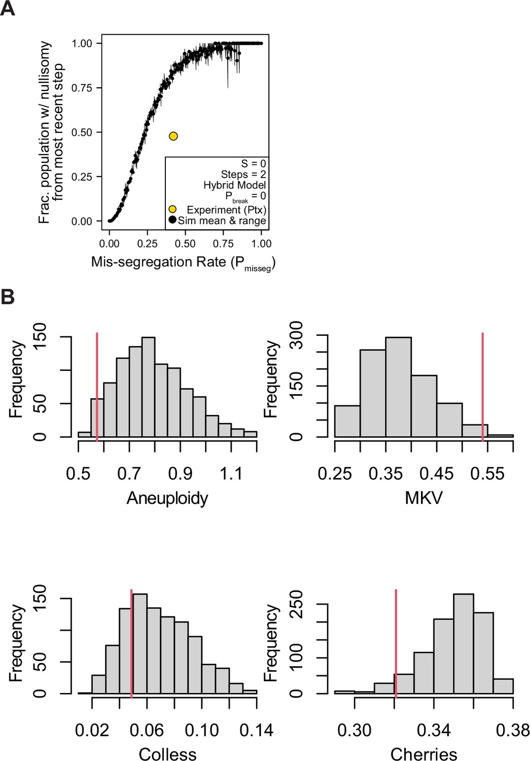
Nullisomy and posterior predictive checks of summary statistics from paclitaxel-treated Cal51 cells.
(A) Observed incidence of nullisomy in paclitaxel-treated cells plotted against the observed mis-segregation rate (Pmisseg,true = 18.5/44 = 0.42) overlaid on simulated data from the second time step (2 generations) under the Hybrid model with S = 0 and Pbreak = 0 (n = 3 simulations). (B) Posterior distributions of summary statistics from accepted simulations most similar to the paclitaxel-treated Cal51 cells (threshold = 0.05). The red line indicates the observed statistic in paclitaxel-treated cells. Colless index and cherry count is normalized to population size. MKV is normalized to the average ploidy of the population.
Figure 5—figure supplement 5
Minimum sampling of karyotype heterogeneity.
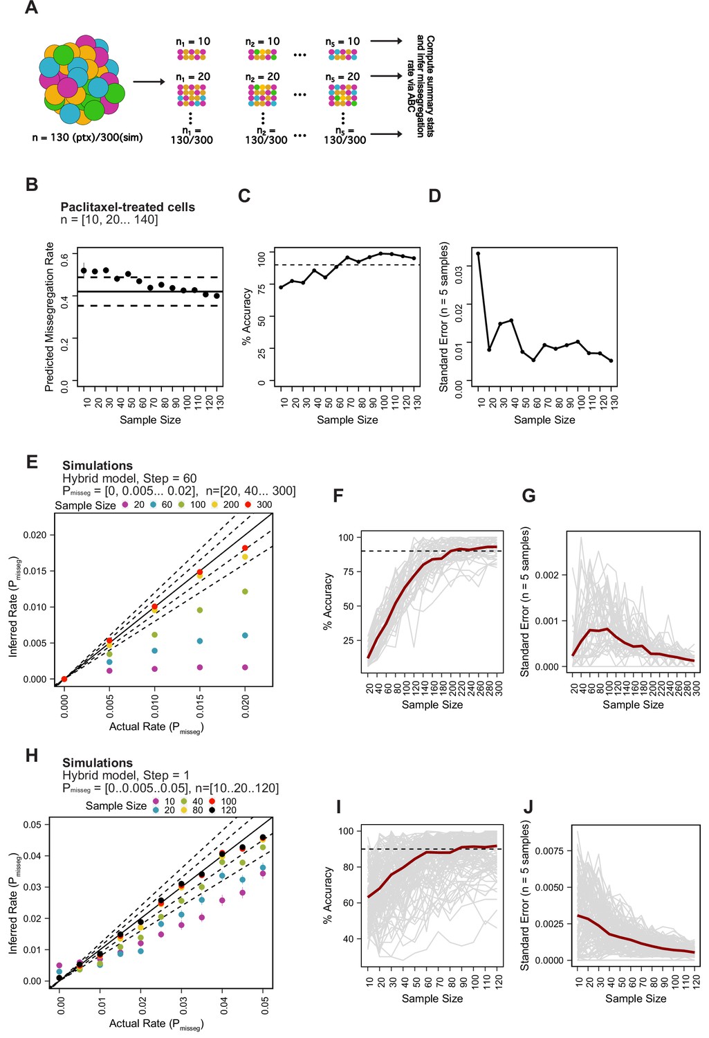
(A) Analytical scheme to optimize the number of cells to sample for measuring mis-segregation rates from karyotype heterogeneity. We iteratively re-sampled and remeasured the rate of mis-segregation for a range of sample sizes (n = 5 random samples). (B) Predicted mis-segregation rates over a range of sample sizes (n = 5 samples). Points and error bars are the mean ± standard error. Black solid line denotes the mean observed rate of mis-segregation induced by 20 nM paclitaxel. Black dashed lines are half the standard deviation of observed mis-segregation rates per cell. (C) Mean percent accuracy of ABC-inferred rates of mis-segregation due to paclitaxel taken from each set of five random samples using the observed rate of mis-segregation as the ‘true value’. Calculated as . Dashed lines represent 90% accuracy. (D) Standard error of ABC-inferred rates of mis-segregation for each set of random samples from paclitaxel-treated cells. (E) ABC-inferred mis-segregation rates by sample size from simulations with known parameters (n = 5 samples). Points represent mean ± standard error across 5 samples for each of 11 selective pressure (S) values. Solid line represents a perfect correlation. Inner dashed line represent ±10% margin. Outer dashed line represents ±20% margin. Simulation parameters: Pmisseg∈ [0, 0.005… 0.02], time steps = 60, Selection Model = ‘Hybrid’, Growth Model = ‘exponential pseudo-Moran’, S = [0, 10... 100], and a tolerance threshold of 0.05. (F) Mean percent accuracy of ABC-inferred rates of mis-segregation in simulations (parameters in E) taken at various sample sizes. Gray lines represent the mean percent accuracy of five random samples for each sample size for the same simulated population (n = 55 simulations). The dashed line represents 90% accuracy. Calculated as described above but taking the known simulation parameter as the ‘true’ value. (G) Standard error of ABC-inferred rates of mis-segregation in simulations (parameters in E) taken at various sample sizes. Gray lines represent the standard error of five random samples for each sample size for the same simulated population (n = 55 simulations). (H) ABC-inferred mis-segregation rates by sample size from simulations with known parameters (n = 5 samples). Points represent mean ± standard error across 5 samples for each of 11 selective pressure (S) values. Solid line represents a perfect correlation. Inner dashed line represent ±10% margin. Outer dashed line represents ±20% margin. ABC was performed with the following parameters and priors: Pmisseg∈[0, 0.005… 0.05], time steps = 1, Selection Model = ‘Hybrid’, Growth Model = ‘exponential pseudo-Moran’, S ∈ [0, 10… 100], and a tolerance threshold of 0.05. (I) Mean percent accuracy of ABC-inferred rates of mis-segregation in simulations (parameters in H) taken at various sample sizes. Gray lines represent the mean percent accuracy of five random samples for each sample size for the same simulated population (n = 121 simulations). The dashed line represents 90% accuracy. (J) Standard error of ABC-inferred rates of mis-segregation in simulations (parameters in H) taken at various sample sizes. Gray lines represent the standard error of five random samples for each sample size for the same simulated population (n = 121 simulations). Note: Red lines in F, G, I, and J represent the median.
Figure 6 with 5 supplements
Inferring chromosome mis-segregation rates in tumors and organoids Bolhaqueiro et al., 2019Navin et al., 2011.
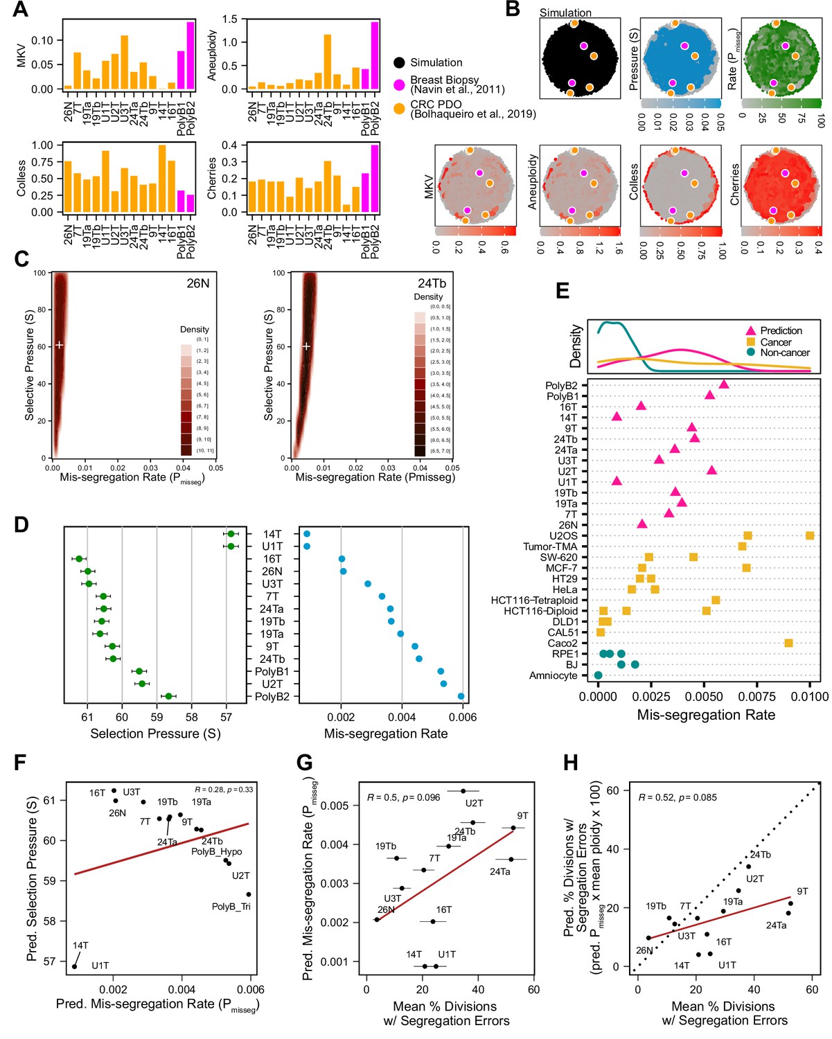
(A) Computed population summary statistics for colorectal cancer (CRC) patient-derived organoids (PDOs) and breast biopsy scDNAseq datasets from Bolhaqueiro et al., 2019 (gold) and Navin et al., 2011 (pink). (B) Dimensionality reduction analysis of population summary statistics showing biological observations overlaid on, and found within, the space of simulated observations. Point colors show the simulation parameters and summary statistics for all simulations using the following priors and parameters: Growth Model = ‘exponential pseudo-Moran’, Selection Model = ‘Abundance’, initial ploidy = 2, time steps ∈[40, 41… 80], S ∈[0,2… 100], Pmisseg∈[0,0.001… 0.050] and a tolerance threshold of 0.05 to reject dissimilar simulation results. (see Materials and Methods). (C) 2D density plots showing joint posterior distributions of Pmisseg and S values from the approximate Bayesian computation analysis of samples 26 N (left) and 24Tb (right) from Bolhaqueiro et al., 2019. White + represents the mean of inferred values. (D) Inferred selective pressures and mis-segregation rates from each scDNAseq dataset (mean and SEM of accepted values). (E) Predicted mis-segregation rates in CRC PDOs and a breast biopsy plotted with approximated mis-segregation rates observed in cancer (blue triangle) and non-cancer (red circle) models (primarily cell lines) from previous studies (Table 5; see Materials and methods). The predicted mis-segregation rates in these cancer-derived samples fall within those observed in cancer cell lines and above those of non-cancer cell lines. (F) Pearson correlation of predicted mis-segregation rates and predicted selective pressures in CRC PDOs from Bolhaqueiro et al., 2019. (G) Pearson correlation of predicted mis-segregation rates and the incidence of observed segregation errors in CRC PDOs from Bolhaqueiro et al., 2019. Error bars represent SEM values. (H) Pearson correlation of observed incidence of segregation errors in CRC PDOs from Bolhaqueiro et al., 2019 to the ploidy-corrected prediction of the observed incidence of segregation errors. These values assume the involvement of 1 chromosome per observed error and are calculated as the (predicted mis-segregation rate) x (mean number of chromosomes observed per cell) x 100. Dotted line = 1:1 reference.
Figure 6—figure supplement 1
ABC-inference threshold and step-window analysis.
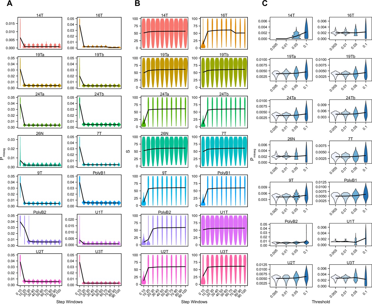
Posterior distributions of mis-segregation rates (A) and selective pressure, S (B) inferred using ABC analysis of CRC organoids and a breast biopsy from Bolhaqueiro et al., 2019 and Navin et al., 2011 respectively using a sliding window prior distribution of time steps. ABC was performed for every interval of 10 steps between 0 and 100 using a tolerance threshold of 0.05. Schematic of analysis shown below. ABC was performed with the following parameters and priors: Pmisseg∈ [0...0.001...0.05], S ∈ [0...2...100], indicated time step window, Selection Model = ‘Abundance’, Growth Model = ‘exponential pseudo-Moran’, and a tolerance threshold of 0.05. (C) Posterior distributions of mis-segregation rates inferred using ABC analysis on the same samples as in A using tolerance thresholds of 0.005, 0.01, 0.05, 0.1. ABC was performed with the following parameters and priors: Pmisseg∈ [0, 0.001… 0.05], S ∈ [0, 2… 100], time steps ∈ [40, 41… 80], Selection Model = ‘Abundance’, Growth Model = ‘exponential pseudo-Moran’, and the indicated tolerance threshold.
Figure 6—figure supplement 2
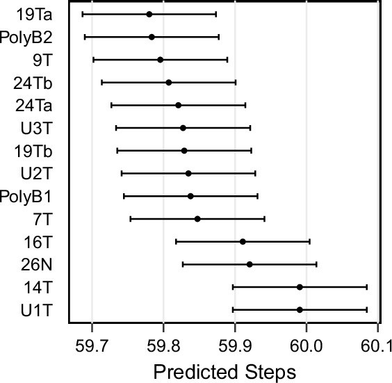
ABC-inferred step count in patient-derived samples.
Mean and standard error for steps in each patient-derived sample (accompanying data in Figure 6), inferred via approximate Bayesian computation.
Figure 6—figure supplement 3
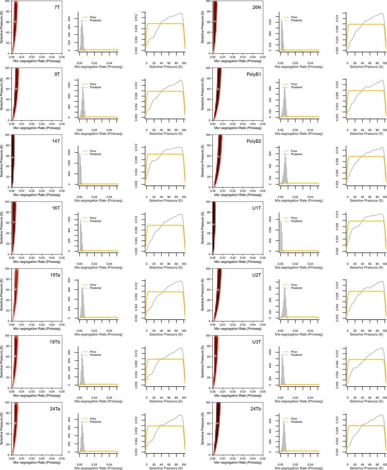
ABC-inferred mis-segregation rates and selective pressures in patient-derived samples.
Joint (2D density plots) and individual (1D density plots) distributions of mis-segregation rates and selective pressures in patient-derived CRC organoids and a breast biopsy from Bolhaqueiro et al., 2019 and Navin et al., 2011 respectively (accompanying data in Figure 6). The prior (yellow) distribution represents the parameters used for simulation while the posterior (gray) distribution represents the parameters from simulations whose observed measurements were similar to the measurements taken from the patient-derived sample using a tolerance threshold of 0.05. White + signs on joint distributions represent the mean of both parameters.
Figure 6—figure supplement 4
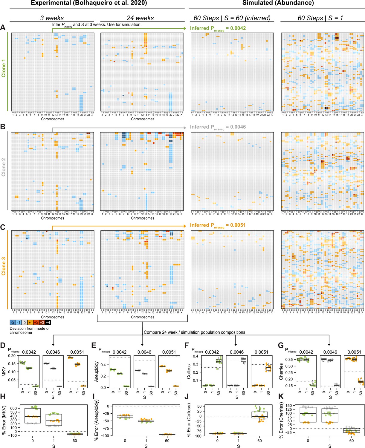
Validation of selection in longitudinally sequenced CRC organoids.
(A–C) Copy number heatmaps showing the deviation from the mode of each chromosome derived from longitudinally sequenced clonal organoids from Bolhaqueiro et al., 2019. ABC was performed on scDNAseq data from three clones at 3 weeks of growth. The resulting inferred mis-segregation rate (Pmisseg) and selective pressure (S) were used to simulate CIN and selection in these clones over 60 time steps, at which point the composition of the populations were compared to the scDNAseq data from each of the clones at 24 weeks of growth (D–K). Additional simulations using S = 0 (not shown) and S = 1 were also performed. Inferred Pmisseg values for (A) clone 1, (B) clone 2, and (C) clone 3 were 0.0042, 0.0046, and 0.0051 respectively. S = 60 was inferred for each clone. ABC was performed on the 3 week data with the following parameters and priors: Pmisseg∈ [0, 0.001... 0.05], S ∈ [0, 2… 100], time steps ∈ [40, 41... 80], Selection Model = ‘Abundance’, Growth Model = ‘exponential pseudo-Moran’, and a tolerance threshold of 0.05. (D) MKV values from n = 10 simulations per clone. Dotted line represents the MKV value observed in the scDNAseq data. (E) Aneuploidy values from n = 10 simulations per clone per S value. Dotted line represents the Aneuploidy value observed in the scDNAseq data. (F) Colless index values from n = 10 simulations per clone S value. Dotted line represents the Colless index value observed in the scDNAseq data. (G) Normalized cherry values from n = 10 simulations per clone S value. Dotted line represents the normalized cherry value observed in the scDNAseq data. (H) Percent error for MKV observations in n = 10 simulations per clone per S value. Dotted line represents 0% error. (I) Percent error for aneuploidy observations in n = 10 simulations per clone per S value. Dotted line represents 0% error. (J) Percent error for Colless observations in n = 10 simulations per clone per S value. Dotted line represents 0% error. (K) Percent error for normalized cherry observations in n = 10 simulations per clone per S value. Dotted line represents 0% error.
Figure 6—figure supplement 5
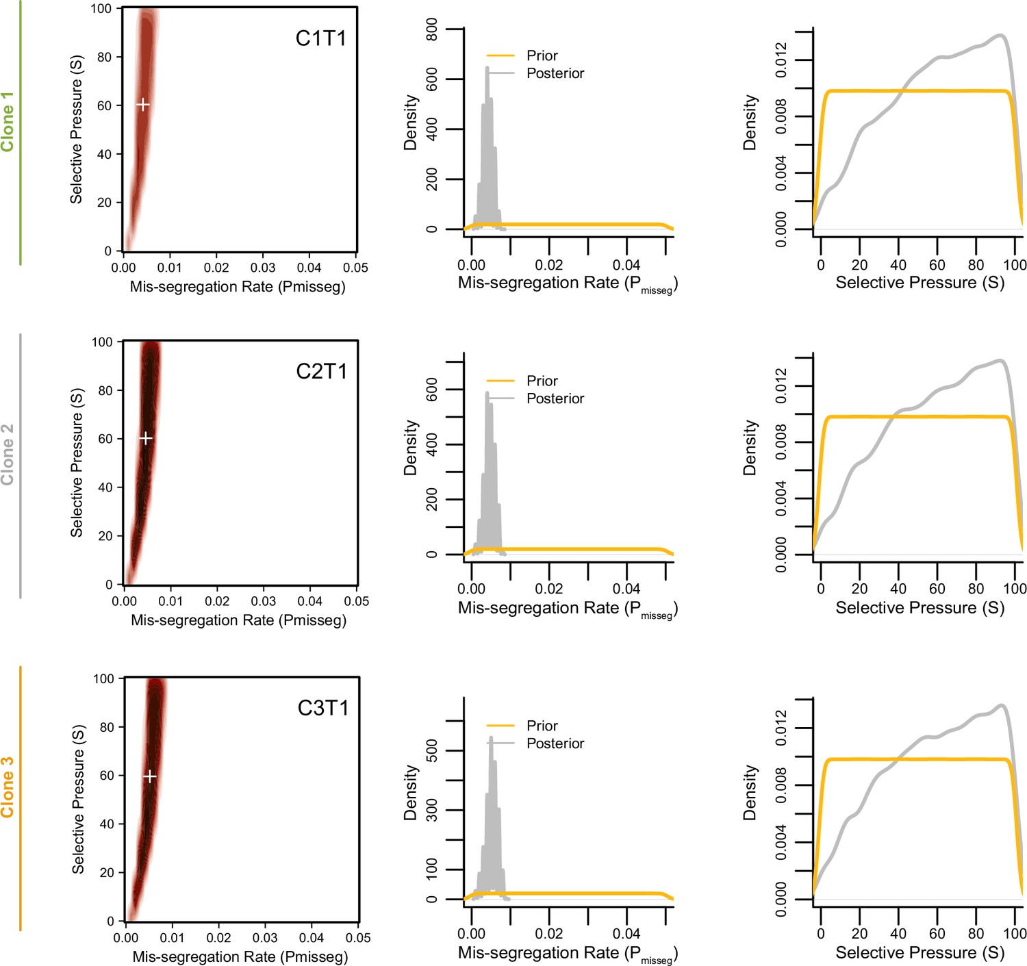
Joint posterior distributions from CRC organoids at 3 weeks.
Joint (2D density plots) and individual (1D density plots) distributions of mis-segregation rates and selective pressures in individual clones of a patient-derived CRC organoid line from Bolhaqueiro et al., 2019 after 3 weeks of growth (accompanying data in Figure 6—figure supplement 4). The prior (yellow) distribution represents the parameters used for simulation while the posterior (gray) distribution represents the parameters from simulations whose observed measurements were similar to the measurements taken from the patient-derived sample using a tolerance threshold of 0.05. White + signs on joint distributions represent the mean of both parameters.
Tables
Table 1
Base chromosome-specific fitness scores for individual models.
| Selection model | |||
|---|---|---|---|
| CHR ARM | Gene Abundance | Driver Density | Hybrid |
| 1p | 0.04780162 | –0.0024018 | 0.02269992 |
| 1q | 0.04340321 | 0.03244362 | 0.03792341 |
| 2p | 0.02733655 | 0.02935717 | 0.02834686 |
| 2q | 0.04244054 | 0.03943267 | 0.0409366 |
| 3p | 0.02310412 | 0.03289695 | 0.02800053 |
| 3q | 0.0299756 | 0.05416736 | 0.04207148 |
| 4p | 0.01238195 | 0.01784909 | 0.01511552 |
| 4q | 0.03181796 | 0.02901324 | 0.0304156 |
| 5p | 0.01178443 | 0.04281166 | 0.02729805 |
| 5q | 0.03787615 | 0.01949934 | 0.02868775 |
| 6p | 0.02557719 | 0.02398619 | 0.02478169 |
| 6q | 0.02554399 | 0.00011625 | 0.01283012 |
| 7p | 0.0179588 | 0.09889284 | 0.05842582 |
| 7q | 0.03231589 | 0.06933314 | 0.05082451 |
| 8p | 0.01591728 | 0.02769564 | 0.02180646 |
| 8q | 0.0254942 | 0.05861427 | 0.04205423 |
| 9p | 0.01301266 | –0.0012941 | 0.00585929 |
| 9q | 0.02572657 | 0.04702681 | 0.03637669 |
| 10 p | 0.0112201 | –0.0364218 | –0.0126008 |
| 10q | 0.02750253 | 0.01142688 | 0.01946471 |
| 11 p | 0.01961858 | 0.03818621 | 0.0289024 |
| 11q | 0.03629936 | 0.01898784 | 0.0276436 |
| 12 p | 0.0142575 | 0.0551551 | 0.0347063 |
| 12q | 0.03659812 | 0.06273786 | 0.04966799 |
| 13 p | 0 | 0 | 0 |
| 13q | 0.02333649 | –0.0101539 | 0.00659128 |
| 14 p | 1.66E-05 | 0 | 8.30E-06 |
| 14q | 0.03792594 | 0.02557439 | 0.03175016 |
| 15 p | 0 | 0 | 0 |
| 15q | 0.03701306 | 0.0206566 | 0.02883483 |
| 16 p | 0.02383442 | 0.04334736 | 0.03359089 |
| 16q | 0.01900446 | –0.0071444 | 0.00593005 |
| 17 p | 0.01548573 | –0.0085975 | 0.00344414 |
| 17q | 0.03553586 | 0.04363474 | 0.0395853 |
| 18 p | 0.00627396 | 0.00533697 | 0.00580547 |
| 18q | 0.01434049 | –0.0263632 | –0.0060113 |
| 19 p | 0.02159372 | 0.05371416 | 0.03765394 |
| 19q | 0.02813325 | 0.00550338 | 0.01681831 |
| 20 p | 0.0089628 | 0.04351025 | 0.02623653 |
| 20q | 0.01526996 | 0.04993593 | 0.03260295 |
| 21 p | 0.00232369 | 0 | 0.00116185 |
| 21q | 0.01233215 | –0.0033092 | 0.00451147 |
| 22 p | 0.00013278 | 0 | 6.64E-05 |
| 22q | 0.02297134 | –0.0051581 | 0.0089066 |
| Xp | 0.01555213 | 0 | 0.00777606 |
| Xp | 0.02499627 | 0 | 0.01249813 |
Table 2
Parameters varied during agent-based modeling.
| Parameter | Description |
|---|---|
| Pmisseg | Probability of mis-segregation per chromosome per division |
| Pbreak | Probability of chromosome breakage after mis-segregation |
| Pdivision | Probability of cellular division per time step |
| S | Magnitude of selective pressure on aneuploid karyotypes |
Table 3
Model selection.
| Sample | Growt Model | Selectio Model | PP | BF (Ho Neutral) | Pmisseg | S | Steps |
|---|---|---|---|---|---|---|---|
| 7T | exponential pseudo-Moran | Abundance | 0.621 | Inf | 0.0033 ± 1e-05 | 60.5416 ± 0.2053 | 59.8475 ± 0.0937 |
| 7T | exponential pseudo-Moran | Driver | 0.14 | Inf | 0.001 ± 1e-05 | 49.6557 ± 0.2389 | 58.7002 ± 0.0943 |
| 7T | exponential pseudo-Moran | Hybrid | 0.239 | Inf | 8e-04 ± 1e-05 | 49.3428 ± 0.2377 | 58.5789 ± 0.0935 |
| 7T | exponential pseudo-Moran | Neutral | 0 | NA | 9e-04 ± 5e-05 | 0 ± 0 | 57.7994 ± 0.6728 |
| 7T | constant Wright-Fisher | Abundance | 0.985 | Inf | 0.0062 ± 2e-05 | 69.7026 ± 0.1724 | 59.9318 ± 0.0937 |
| 7T | constant Wright-Fisher | Driver | 0 | NA | 0.0012 ± 1e-05 | 48.2881 ± 0.2384 | 57.5239 ± 0.0933 |
| 7T | constant Wright-Fisher | Hybrid | 0.015 | Inf | 9e-04 ± 1e-05 | 50.7803 ± 0.2359 | 58.2514 ± 0.0941 |
| 7T | constant Wright-Fisher | Neutral | 0 | NA | 9e-04 ± 5e-05 | 0 ± 0 | 58.7803 ± 0.6701 |
| U1T | exponential pseudo-Moran | Abundance | 0.582 | 199 | 9e-04 ± 1e-05 | 56.8672 ± 0.2168 | 59.9906 ± 0.0937 |
| U1T | exponential pseudo-Moran | Driver | 0.113 | 39 | 0.001 ± 1e-05 | 49.6611 ± 0.2389 | 58.6886 ± 0.0944 |
| U1T | exponential pseudo-Moran | Hybrid | 0.156 | 54 | 8e-04 ± 1e-05 | 49.3658 ± 0.2375 | 58.569 ± 0.0935 |
| U1T | exponential pseudo-Moran | Neutral | 0.149 | 1 | 9e-04 ± 5e-05 | 0 ± 0 | 57.7102 ± 0.67 |
| U1T | constant Wright-Fisher | Abundance | 0.654 | 290 | 0.001 ± 1e-05 | 61.4358 ± 0.2029 | 60.0021 ± 0.0937 |
| U1T | constant Wright-Fisher | Driver | 0.115 | 51 | 0.0012 ± 1e-05 | 48.2767 ± 0.2383 | 57.5267 ± 0.0934 |
| U1T | constant Wright-Fisher | Hybrid | 0.115 | 51 | 9e-04 ± 1e-05 | 50.8033 ± 0.2358 | 58.2507 ± 0.0941 |
| U1T | constant Wright-Fisher | Neutral | 0.115 | 1 | 9e-04 ± 5e-05 | 0 ± 0 | 58.7803 ± 0.6701 |
| U2T | exponential pseudo-Moran | Abundance | 0.628 | 251 | 0.0054 ± 1e-05 | 59.4269 ± 0.2108 | 59.8349 ± 0.0935 |
| U2T | exponential pseudo-Moran | Driver | 0.079 | 32 | 0.0027 ± 2e-05 | 50.1513 ± 0.2396 | 57.4538 ± 0.0934 |
| U2T | exponential pseudo-Moran | Hybrid | 0.166 | 66 | 0.0022 ± 2e-05 | 48.7779 ± 0.2413 | 57.7078 ± 0.0934 |
| U2T | exponential pseudo-Moran | Neutral | 0.127 | 1 | 0.0021 ± 7e-05 | 0 ± 0 | 56.8535 ± 0.6619 |
| U2T | constant Wright-Fisher | Abundance | 0.918 | 2817 | 0.0112 ± 3e-05 | 69.7222 ± 0.1703 | 60.0655 ± 0.0934 |
| U2T | constant Wright-Fisher | Driver | 0.001 | 4 | 0.0027 ± 2e-05 | 48.7794 ± 0.2389 | 56.4812 ± 0.0919 |
| U2T | constant Wright-Fisher | Hybrid | 0.064 | 196 | 0.0022 ± 1e-05 | 50.9564 ± 0.2379 | 57.1161 ± 0.0925 |
| U2T | constant Wright-Fisher | Neutral | 0.017 | 1 | 0.0022 ± 1e-04 | 0 ± 0 | 57.7898 ± 0.6841 |
| U3T | exponential pseudo-Moran | Abundance | 0.582 | 199 | 0.0029 ± 1e-05 | 60.9557 ± 0.2091 | 59.8273 ± 0.0938 |
| U3T | exponential pseudo-Moran | Driver | 0.113 | 39 | 0.001 ± 1e-05 | 49.6707 ± 0.2389 | 58.6986 ± 0.0944 |
| U3T | exponential pseudo-Moran | Hybrid | 0.156 | 54 | 8e-04 ± 1e-05 | 49.3754 ± 0.2376 | 58.5711 ± 0.0935 |
| U3T | exponential pseudo-Moran | Neutral | 0.149 | 1 | 9e-04 ± 5e-05 | 0 ± 0 | 57.7102 ± 0.67 |
| U3T | constant Wright-Fisher | Abundance | 0.736 | Inf | 0.0052 ± 2e-05 | 69.8357 ± 0.1713 | 59.932 ± 0.0934 |
| U3T | constant Wright-Fisher | Driver | 0.13 | Inf | 0.0012 ± 1e-05 | 48.2864 ± 0.2383 | 57.5385 ± 0.0934 |
| U3T | constant Wright-Fisher | Hybrid | 0.134 | Inf | 9e-04 ± 1e-05 | 50.8219 ± 0.2357 | 58.2482 ± 0.0941 |
| U3T | constant Wright-Fisher | Neutral | 0 | NA | 9e-04 ± 5e-05 | 0 ± 0 | 58.8567 ± 0.6676 |
| 14T | exponential pseudo-Moran | Abundance | 0.582 | 199 | 9e-04 ± 1e-05 | 56.8672 ± 0.2168 | 59.9906 ± 0.0937 |
| 14T | exponential pseudo-Moran | Driver | 0.113 | 39 | 0.001 ± 1e-05 | 49.6614 ± 0.239 | 58.695 ± 0.0944 |
| 14T | exponential pseudo-Moran | Hybrid | 0.156 | 54 | 8e-04 ± 1e-05 | 49.3716 ± 0.2375 | 58.5632 ± 0.0935 |
| 14T | exponential pseudo-Moran | Neutral | 0.149 | 1 | 9e-04 ± 5e-05 | 0 ± 0 | 57.7102 ± 0.67 |
| 14T | constant Wright-Fisher | Abundance | 0.654 | 290 | 0.0011 ± 1e-05 | 62.8579 ± 0.2075 | 60.0029 ± 0.0936 |
| 14T | constant Wright-Fisher | Driver | 0.115 | 51 | 0.0012 ± 1e-05 | 48.2967 ± 0.2383 | 57.5295 ± 0.0934 |
| 14T | constant Wright-Fisher | Hybrid | 0.115 | 51 | 9e-04 ± 1e-05 | 50.8274 ± 0.2357 | 58.2478 ± 0.0941 |
| 14T | constant Wright-Fisher | Neutral | 0.115 | 1 | 9e-04 ± 5e-05 | 0 ± 0 | 58.8567 ± 0.6676 |
| 16T | exponential pseudo-Moran | Abundance | 0.582 | 199 | 0.002 ± 1e-05 | 61.2401 ± 0.2028 | 59.9109 ± 0.0935 |
| 16T | exponential pseudo-Moran | Driver | 0.113 | 39 | 0.001 ± 1e-05 | 49.6539 ± 0.2389 | 58.7006 ± 0.0943 |
| 16T | exponential pseudo-Moran | Hybrid | 0.156 | 54 | 8e-04 ± 1e-05 | 49.3611 ± 0.2376 | 58.574 ± 0.0935 |
| 16T | exponential pseudo-Moran | Neutral | 0.149 | 1 | 9e-04 ± 5e-05 | 0 ± 0 | 57.7994 ± 0.6728 |
| 16T | constant Wright-Fisher | Abundance | 0.654 | 290 | 0.0038 ± 1e-05 | 69.8456 ± 0.1701 | 59.9523 ± 0.0936 |
| 16T | constant Wright-Fisher | Driver | 0.115 | 51 | 0.0012 ± 1e-05 | 48.261 ± 0.2384 | 57.5233 ± 0.0933 |
| 16T | constant Wright-Fisher | Hybrid | 0.115 | 51 | 9e-04 ± 1e-05 | 50.7713 ± 0.2359 | 58.2554 ± 0.0941 |
| 16T | constant Wright-Fisher | Neutral | 0.115 | 1 | 9e-04 ± 5e-05 | 0 ± 0 | 58.7803 ± 0.6701 |
| 19Ta | exponential pseudo-Moran | Abundance | 0.711 | 313 | 0.004 ± 1e-05 | 60.6391 ± 0.2074 | 59.7801 ± 0.0934 |
| 19Ta | exponential pseudo-Moran | Driver | 0.038 | 17 | 0.0028 ± 2e-05 | 50.2185 ± 0.2399 | 57.3764 ± 0.0934 |
| 19Ta | exponential pseudo-Moran | Hybrid | 0.135 | 59 | 0.0022 ± 3e-05 | 48.3823 ± 0.242 | 57.5368 ± 0.0935 |
| 19Ta | exponential pseudo-Moran | Neutral | 0.116 | 1 | 0.0022 ± 9e-05 | 0 ± 0 | 56.5955 ± 0.6549 |
| 19Ta | constant Wright-Fisher | Abundance | 0.97 | 11760 | 0.0075 ± 2e-05 | 69.3863 ± 0.1735 | 59.956 ± 0.0938 |
| 19Ta | constant Wright-Fisher | Driver | 0 | 0 | 0.0028 ± 2e-05 | 48.8413 ± 0.2392 | 56.4529 ± 0.0917 |
| 19Ta | constant Wright-Fisher | Hybrid | 0.026 | 315 | 0.0023 ± 1e-05 | 50.8588 ± 0.2383 | 57.1031 ± 0.0925 |
| 19Ta | constant Wright-Fisher | Neutral | 0.004 | 1 | 0.0023 ± 1e-04 | 0 ± 0 | 57.9522 ± 0.6869 |
| 19Tb | exponential pseudo-Moran | Abundance | 0.727 | 320 | 0.0036 ± 1e-05 | 60.5885 ± 0.2085 | 59.829 ± 0.0938 |
| 19Tb | exponential pseudo-Moran | Driver | 0.03 | 13 | 0.001 ± 1e-05 | 49.6622 ± 0.2389 | 58.6929 ± 0.0944 |
| 19Tb | exponential pseudo-Moran | Hybrid | 0.127 | 56 | 8e-04 ± 1e-05 | 48.5237 ± 0.2322 | 58.9663 ± 0.0931 |
| 19Tb | exponential pseudo-Moran | Neutral | 0.116 | 1 | 9e-04 ± 5e-05 | 0 ± 0 | 57.7102 ± 0.67 |
| 19Tb | constant Wright-Fisher | Abundance | 0.979 | 47320 | 0.0068 ± 2e-05 | 69.5697 ± 0.173 | 59.9232 ± 0.0935 |
| 19Tb | constant Wright-Fisher | Driver | 0 | 0 | 0.0012 ± 1e-05 | 48.2786 ± 0.2383 | 57.5433 ± 0.0934 |
| 19Tb | constant Wright-Fisher | Hybrid | 0.02 | 982 | 9e-04 ± 1e-05 | 50.8162 ± 0.2357 | 58.2495 ± 0.0941 |
| 19Tb | constant Wright-Fisher | Neutral | 0.001 | 1 | 9e-04 ± 5e-05 | 0 ± 0 | 58.8376 ± 0.669 |
| 24Ta | exponential pseudo-Moran | Abundance | 0.731 | 321 | 0.0036 ± 1e-05 | 60.5303 ± 0.2082 | 59.8208 ± 0.0938 |
| 24Ta | exponential pseudo-Moran | Driver | 0.029 | 13 | 0.001 ± 1e-05 | 49.6703 ± 0.2389 | 58.6938 ± 0.0944 |
| 24Ta | exponential pseudo-Moran | Hybrid | 0.125 | 55 | 8e-04 ± 1e-05 | 49.3669 ± 0.2376 | 58.5778 ± 0.0935 |
| 24Ta | exponential pseudo-Moran | Neutral | 0.116 | 1 | 9e-04 ± 5e-05 | 0 ± 0 | 57.7102 ± 0.67 |
| 24Ta | constant Wright-Fisher | Abundance | 0.979 | 47346 | 0.0068 ± 2e-05 | 69.6173 ± 0.173 | 59.933 ± 0.0934 |
| 24Ta | constant Wright-Fisher | Driver | 0 | 0 | 0.0012 ± 1e-05 | 48.2789 ± 0.2383 | 57.5377 ± 0.0934 |
| 24Ta | constant Wright-Fisher | Hybrid | 0.02 | 956 | 9e-04 ± 1e-05 | 50.8229 ± 0.2357 | 58.2524 ± 0.0941 |
| 24Ta | constant Wright-Fisher | Neutral | 0.001 | 1 | 9e-04 ± 5e-05 | 0 ± 0 | 58.8567 ± 0.6676 |
| 24Tb | exponential pseudo-Moran | Abundance | 0.68 | 294 | 0.0046 ± 1e-05 | 60.2602 ± 0.2084 | 59.8073 ± 0.0936 |
| 24Tb | exponential pseudo-Moran | Driver | 0.054 | 23 | 0.0031 ± 3e-05 | 50.2981 ± 0.2399 | 57.2927 ± 0.0934 |
| 24Tb | exponential pseudo-Moran | Hybrid | 0.149 | 65 | 0.0025 ± 4e-05 | 48.3833 ± 0.244 | 57.4236 ± 0.0936 |
| 24Tb | exponential pseudo-Moran | Neutral | 0.118 | 1 | 0.0025 ± 0.00013 | 0 ± 0 | 56.7229 ± 0.6579 |
| 24Tb | constant Wright-Fisher | Abundance | 0.954 | 7730 | 0.0215 ± 0.00011 | 33.6703 ± 0.2962 | 59.9064 ± 0.0937 |
| 24Tb | constant Wright-Fisher | Driver | 0 | 2 | 0.003 ± 2e-05 | 48.7528 ± 0.2393 | 56.4175 ± 0.0918 |
| 24Tb | constant Wright-Fisher | Hybrid | 0.039 | 318 | 0.0024 ± 2e-05 | 50.7006 ± 0.2389 | 57.107 ± 0.0925 |
| 24Tb | constant Wright-Fisher | Neutral | 0.006 | 1 | 0.0024 ± 0.00011 | 0 ± 0 | 58.0318 ± 0.6822 |
| 26N | exponential pseudo-Moran | Abundance | 0.582 | 199 | 0.0021 ± 1e-05 | 60.9877 ± 0.2031 | 59.9205 ± 0.0934 |
| 26N | exponential pseudo-Moran | Driver | 0.113 | 39 | 0.001 ± 1e-05 | 49.6389 ± 0.2389 | 58.7018 ± 0.0944 |
| 26N | exponential pseudo-Moran | Hybrid | 0.156 | 54 | 8e-04 ± 1e-05 | 49.3389 ± 0.2377 | 58.5755 ± 0.0935 |
| 26N | exponential pseudo-Moran | Neutral | 0.149 | 1 | 9e-04 ± 5e-05 | 0 ± 0 | 57.7994 ± 0.6728 |
| 26N | constant Wright-Fisher | Abundance | 0.654 | 290 | 0.0039 ± 1e-05 | 69.794 ± 0.1704 | 59.9547 ± 0.0935 |
| 26N | constant Wright-Fisher | Driver | 0.115 | 51 | 0.0012 ± 1e-05 | 48.2849 ± 0.2384 | 57.5175 ± 0.0933 |
| 26N | constant Wright-Fisher | Hybrid | 0.115 | 51 | 9e-04 ± 1e-05 | 50.737 ± 0.2359 | 58.2609 ± 0.0941 |
| 26N | constant Wright-Fisher | Neutral | 0.115 | 1 | 9e-04 ± 5e-05 | 0 ± 0 | 58.7803 ± 0.6701 |
| 9T | exponential pseudo-Moran | Abundance | 0.685 | 299 | 0.0044 ± 1e-05 | 60.2829 ± 0.2086 | 59.7955 ± 0.0936 |
| 9T | exponential pseudo-Moran | Driver | 0.052 | 23 | 0.0029 ± 2e-05 | 50.2323 ± 0.2398 | 57.3657 ± 0.0934 |
| 9T | exponential pseudo-Moran | Hybrid | 0.147 | 64 | 0.0022 ± 3e-05 | 48.3829 ± 0.2422 | 57.5193 ± 0.0936 |
| 9T | exponential pseudo-Moran | Neutral | 0.117 | 1 | 0.0023 ± 9e-05 | 0 ± 0 | 56.6083 ± 0.6581 |
| 9T | constant Wright-Fisher | Abundance | 0.958 | 9299 | 0.0087 ± 2e-05 | 69.6836 ± 0.1724 | 59.926 ± 0.0937 |
| 9T | constant Wright-Fisher | Driver | 0 | 1 | 0.0028 ± 2e-05 | 48.8394 ± 0.2392 | 56.4465 ± 0.0917 |
| 9T | constant Wright-Fisher | Hybrid | 0.037 | 360 | 0.0023 ± 1e-05 | 50.8477 ± 0.2384 | 57.0952 ± 0.0925 |
| 9T | constant Wright-Fisher | Neutral | 0.005 | 1 | 0.0023 ± 1e-04 | 0 ± 0 | 57.9427 ± 0.687 |
| PolyB1 | exponential pseudo-Moran | Abundance | 0.635 | 261 | 0.0053 ± 1e-05 | 59.5088 ± 0.2104 | 59.8379 ± 0.0935 |
| PolyB1 | exponential pseudo-Moran | Driver | 0.076 | 31 | 0.0028 ± 2e-05 | 50.2364 ± 0.2398 | 57.4025 ± 0.0934 |
| PolyB1 | exponential pseudo-Moran | Hybrid | 0.164 | 67 | 0.0022 ± 3e-05 | 48.6949 ± 0.2419 | 57.6322 ± 0.0934 |
| PolyB1 | exponential pseudo-Moran | Neutral | 0.124 | 1 | 0.0022 ± 9e-05 | 0 ± 0 | 56.5955 ± 0.6549 |
| PolyB1 | constant Wright-Fisher | Abundance | 0.925 | 3482 | 0.0111 ± 3e-05 | 70.2557 ± 0.169 | 60.042 ± 0.0936 |
| PolyB1 | constant Wright-Fisher | Driver | 0.001 | 4 | 0.0028 ± 2e-05 | 48.8194 ± 0.2391 | 56.4451 ± 0.0917 |
| PolyB1 | constant Wright-Fisher | Hybrid | 0.061 | 228 | 0.0023 ± 1e-05 | 50.895 ± 0.2381 | 57.1073 ± 0.0925 |
| PolyB1 | constant Wright-Fisher | Neutral | 0.014 | 1 | 0.0023 ± 1e-04 | 0 ± 0 | 57.9809 ± 0.6861 |
| PolyB2 | exponential pseudo-Moran | Abundance | 0.603 | 218 | 0.0059 ± 1e-05 | 58.6612 ± 0.212 | 59.7835 ± 0.0937 |
| PolyB2 | exponential pseudo-Moran | Driver | 0.086 | 31 | 0.0038 ± 4e-05 | 50.2948 ± 0.2394 | 57.0217 ± 0.093 |
| PolyB2 | exponential pseudo-Moran | Hybrid | 0.17 | 61 | 0.004 ± 7e-05 | 48.9466 ± 0.2472 | 57.28 ± 0.0942 |
| PolyB2 | exponential pseudo-Moran | Neutral | 0.141 | 1 | 0.0033 ± 0.00022 | 0 ± 0 | 56.5732 ± 0.6597 |
| PolyB2 | constant Wright-Fisher | Abundance | 0.893 | 1277 | 0.0301 ± 1e-04 | 3.0543 ± 0.0165 | 59.9142 ± 0.0936 |
| PolyB2 | constant Wright-Fisher | Driver | 0.003 | 4 | 0.0034 ± 3e-05 | 48.7328 ± 0.2396 | 56.3664 ± 0.0917 |
| PolyB2 | constant Wright-Fisher | Hybrid | 0.069 | 98 | 0.0027 ± 2e-05 | 50.3534 ± 0.2405 | 57.1445 ± 0.0928 |
| PolyB2 | constant Wright-Fisher | Neutral | 0.036 | 1 | 0.0026 ± 0.00014 | 0 ± 0 | 58.1592 ± 0.6741 |
Table 4
Model selection with selective pressure constrained to S = 1.
| Sample | Growth Model | Selection Model | PP | BF (Ho Neutral) | Pmisseg | S | Steps |
|---|---|---|---|---|---|---|---|
| 7T | exponential pseudo-Moran | Abundance | 0.274 | 1 | 9e-04 ± 5e-05 | 1 ± 0 | 58.2452 ± 0.6646 |
| 7T | exponential pseudo-Moran | Driver | 0.238 | 1 | 9e-04 ± 5e-05 | 1 ± 0 | 58.4745 ± 0.6725 |
| 7T | exponential pseudo-Moran | Hybrid | 0.26 | 1 | 9e-04 ± 5e-05 | 1 ± 0 | 58.586 ± 0.6668 |
| 7T | exponential pseudo-Moran | Neutral | 0.228 | 1 | 9e-04 ± 6e-05 | 1 ± 0 | 58.5446 ± 0.6791 |
| 7T | constant Wright-Fisher | Abundance | 0.259 | 1 | 9e-04 ± 6e-05 | 1 ± 0 | 58.8089 ± 0.6627 |
| 7T | constant Wright-Fisher | Driver | 0.24 | 1 | 9e-04 ± 6e-05 | 1 ± 0 | 58.1783 ± 0.6771 |
| 7T | constant Wright-Fisher | Hybrid | 0.257 | 1 | 9e-04 ± 5e-05 | 1 ± 0 | 59.0924 ± 0.6742 |
| 7T | constant Wright-Fisher | Neutral | 0.245 | 1 | 9e-04 ± 7e-05 | 1 ± 0 | 58.7516 ± 0.6787 |
| U1T | exponential pseudo-Moran | Abundance | 0.275 | 1 | 9e-04 ± 5e-05 | 1 ± 0 | 58.2452 ± 0.6646 |
| U1T | exponential pseudo-Moran | Driver | 0.239 | 1 | 9e-04 ± 5e-05 | 1 ± 0 | 58.4745 ± 0.6725 |
| U1T | exponential pseudo-Moran | Hybrid | 0.258 | 1 | 9e-04 ± 5e-05 | 1 ± 0 | 58.586 ± 0.6668 |
| U1T | exponential pseudo-Moran | Neutral | 0.228 | 1 | 9e-04 ± 6e-05 | 1 ± 0 | 58.5446 ± 0.6791 |
| U1T | constant Wright-Fisher | Abundance | 0.259 | 1 | 9e-04 ± 6e-05 | 1 ± 0 | 58.8089 ± 0.6627 |
| U1T | constant Wright-Fisher | Driver | 0.24 | 1 | 9e-04 ± 6e-05 | 1 ± 0 | 58.1783 ± 0.6771 |
| U1T | constant Wright-Fisher | Hybrid | 0.257 | 1 | 9e-04 ± 5e-05 | 1 ± 0 | 59.1592 ± 0.6715 |
| U1T | constant Wright-Fisher | Neutral | 0.245 | 1 | 9e-04 ± 7e-05 | 1 ± 0 | 58.7516 ± 0.6787 |
| U2T | exponential pseudo-Moran | Abundance | 0.276 | 1 | 0.0021 ± 8e-05 | 1 ± 0 | 57.3057 ± 0.653 |
| U2T | exponential pseudo-Moran | Driver | 0.235 | 1 | 0.0024 ± 0.00011 | 1 ± 0 | 57.7452 ± 0.6634 |
| U2T | exponential pseudo-Moran | Hybrid | 0.264 | 1 | 0.0021 ± 7e-05 | 1 ± 0 | 58.1274 ± 0.654 |
| U2T | exponential pseudo-Moran | Neutral | 0.225 | 1 | 0.0024 ± 0.00011 | 1 ± 0 | 57.8758 ± 0.6772 |
| U2T | constant Wright-Fisher | Abundance | 0.269 | 1 | 0.0023 ± 1e-04 | 1 ± 0 | 58.3439 ± 0.6532 |
| U2T | constant Wright-Fisher | Driver | 0.233 | 1 | 0.0023 ± 9e-05 | 1 ± 0 | 57.4777 ± 0.693 |
| U2T | constant Wright-Fisher | Hybrid | 0.263 | 1 | 0.0023 ± 1e-04 | 1 ± 0 | 57.8662 ± 0.6683 |
| U2T | constant Wright-Fisher | Neutral | 0.236 | 1 | 0.0025 ± 0.00012 | 1 ± 0 | 57.1433 ± 0.6655 |
| U3T | exponential pseudo-Moran | Abundance | 0.275 | 1 | 9e-04 ± 5e-05 | 1 ± 0 | 58.1624 ± 0.6643 |
| U3T | exponential pseudo-Moran | Driver | 0.239 | 1 | 9e-04 ± 5e-05 | 1 ± 0 | 58.4554 ± 0.6736 |
| U3T | exponential pseudo-Moran | Hybrid | 0.258 | 1 | 9e-04 ± 5e-05 | 1 ± 0 | 58.586 ± 0.6668 |
| U3T | exponential pseudo-Moran | Neutral | 0.228 | 1 | 9e-04 ± 6e-05 | 1 ± 0 | 58.6178 ± 0.6777 |
| U3T | constant Wright-Fisher | Abundance | 0.259 | 1 | 9e-04 ± 6e-05 | 1 ± 0 | 58.7611 ± 0.6614 |
| U3T | constant Wright-Fisher | Driver | 0.24 | 1 | 9e-04 ± 6e-05 | 1 ± 0 | 58.1783 ± 0.6771 |
| U3T | constant Wright-Fisher | Hybrid | 0.257 | 1 | 9e-04 ± 5e-05 | 1 ± 0 | 59.0955 ± 0.674 |
| U3T | constant Wright-Fisher | Neutral | 0.245 | 1 | 9e-04 ± 7e-05 | 1 ± 0 | 58.7516 ± 0.6787 |
| 14T | exponential pseudo-Moran | Abundance | 0.275 | 1 | 9e-04 ± 5e-05 | 1 ± 0 | 58.1624 ± 0.6643 |
| 14T | exponential pseudo-Moran | Driver | 0.239 | 1 | 9e-04 ± 5e-05 | 1 ± 0 | 58.4554 ± 0.6736 |
| 14T | exponential pseudo-Moran | Hybrid | 0.258 | 1 | 9e-04 ± 5e-05 | 1 ± 0 | 58.586 ± 0.6668 |
| 14T | exponential pseudo-Moran | Neutral | 0.228 | 1 | 9e-04 ± 6e-05 | 1 ± 0 | 58.5446 ± 0.6791 |
| 14T | constant Wright-Fisher | Abundance | 0.259 | 1 | 9e-04 ± 6e-05 | 1 ± 0 | 58.8089 ± 0.6627 |
| 14T | constant Wright-Fisher | Driver | 0.24 | 1 | 9e-04 ± 6e-05 | 1 ± 0 | 58.1783 ± 0.6771 |
| 14T | constant Wright-Fisher | Hybrid | 0.257 | 1 | 9e-04 ± 5e-05 | 1 ± 0 | 59.0924 ± 0.6739 |
| 14T | constant Wright-Fisher | Neutral | 0.245 | 1 | 9e-04 ± 7e-05 | 1 ± 0 | 58.7516 ± 0.6787 |
| 16T | exponential pseudo-Moran | Abundance | 0.274 | 1 | 9e-04 ± 5e-05 | 1 ± 0 | 58.2452 ± 0.6646 |
| 16T | exponential pseudo-Moran | Driver | 0.238 | 1 | 9e-04 ± 5e-05 | 1 ± 0 | 58.4745 ± 0.6725 |
| 16T | exponential pseudo-Moran | Hybrid | 0.26 | 1 | 9e-04 ± 5e-05 | 1 ± 0 | 58.586 ± 0.6668 |
| 16T | exponential pseudo-Moran | Neutral | 0.228 | 1 | 0.001 ± 6e-05 | 1 ± 0 | 58.6274 ± 0.6789 |
| 16T | constant Wright-Fisher | Abundance | 0.259 | 1 | 9e-04 ± 6e-05 | 1 ± 0 | 58.8089 ± 0.6627 |
| 16T | constant Wright-Fisher | Driver | 0.24 | 1 | 9e-04 ± 6e-05 | 1 ± 0 | 58.1783 ± 0.6771 |
| 16T | constant Wright-Fisher | Hybrid | 0.257 | 1 | 9e-04 ± 5e-05 | 1 ± 0 | 59.1051 ± 0.6742 |
| 16T | constant Wright-Fisher | Neutral | 0.245 | 1 | 9e-04 ± 7e-05 | 1 ± 0 | 58.7516 ± 0.6787 |
| 19Ta | exponential pseudo-Moran | Abundance | 0.273 | 1 | 0.0021 ± 8e-05 | 1 ± 0 | 57.4045 ± 0.6565 |
| 19Ta | exponential pseudo-Moran | Driver | 0.243 | 1 | 0.0024 ± 0.00011 | 1 ± 0 | 57.8025 ± 0.663 |
| 19Ta | exponential pseudo-Moran | Hybrid | 0.261 | 1 | 0.0022 ± 8e-05 | 1 ± 0 | 57.9108 ± 0.65 |
| 19Ta | exponential pseudo-Moran | Neutral | 0.222 | 1 | 0.0025 ± 0.00012 | 1 ± 0 | 57.9331 ± 0.6777 |
| 19Ta | constant Wright-Fisher | Abundance | 0.27 | 1 | 0.0024 ± 0.00011 | 1 ± 0 | 58.2866 ± 0.6566 |
| 19Ta | constant Wright-Fisher | Driver | 0.233 | 1 | 0.0023 ± 1e-04 | 1 ± 0 | 57.8185 ± 0.6927 |
| 19Ta | constant Wright-Fisher | Hybrid | 0.261 | 1 | 0.0023 ± 1e-04 | 1 ± 0 | 58.0478 ± 0.6705 |
| 19Ta | constant Wright-Fisher | Neutral | 0.237 | 1 | 0.0025 ± 0.00012 | 1 ± 0 | 57.2261 ± 0.6669 |
| 19Tb | exponential pseudo-Moran | Abundance | 0.275 | 1 | 9e-04 ± 5e-05 | 1 ± 0 | 58.1624 ± 0.6643 |
| 19Tb | exponential pseudo-Moran | Driver | 0.239 | 1 | 9e-04 ± 5e-05 | 1 ± 0 | 58.4554 ± 0.6736 |
| 19Tb | exponential pseudo-Moran | Hybrid | 0.258 | 1 | 9e-04 ± 5e-05 | 1 ± 0 | 58.586 ± 0.6668 |
| 19Tb | exponential pseudo-Moran | Neutral | 0.228 | 1 | 9e-04 ± 6e-05 | 1 ± 0 | 58.5796 ± 0.6796 |
| 19Tb | constant Wright-Fisher | Abundance | 0.259 | 1 | 9e-04 ± 6e-05 | 1 ± 0 | 58.7611 ± 0.6614 |
| 19Tb | constant Wright-Fisher | Driver | 0.24 | 1 | 9e-04 ± 6e-05 | 1 ± 0 | 58.1178 ± 0.679 |
| 19Tb | constant Wright-Fisher | Hybrid | 0.257 | 1 | 9e-04 ± 5e-05 | 1 ± 0 | 59.1592 ± 0.6715 |
| 19Tb | constant Wright-Fisher | Neutral | 0.245 | 1 | 9e-04 ± 7e-05 | 1 ± 0 | 58.7516 ± 0.6787 |
| 24Ta | exponential pseudo-Moran | Abundance | 0.275 | 1 | 9e-04 ± 5e-05 | 1 ± 0 | 58.1624 ± 0.6643 |
| 24Ta | exponential pseudo-Moran | Driver | 0.239 | 1 | 9e-04 ± 5e-05 | 1 ± 0 | 58.4554 ± 0.6736 |
| 24Ta | exponential pseudo-Moran | Hybrid | 0.258 | 1 | 9e-04 ± 5e-05 | 1 ± 0 | 58.586 ± 0.6668 |
| 24Ta | exponential pseudo-Moran | Neutral | 0.228 | 1 | 9e-04 ± 6e-05 | 1 ± 0 | 58.6656 ± 0.6783 |
| 24Ta | constant Wright-Fisher | Abundance | 0.259 | 1 | 9e-04 ± 6e-05 | 1 ± 0 | 58.7611 ± 0.6614 |
| 24Ta | constant Wright-Fisher | Driver | 0.24 | 1 | 9e-04 ± 6e-05 | 1 ± 0 | 58.1783 ± 0.6771 |
| 24Ta | constant Wright-Fisher | Hybrid | 0.257 | 1 | 9e-04 ± 5e-05 | 1 ± 0 | 59.1592 ± 0.6715 |
| 24Ta | constant Wright-Fisher | Neutral | 0.245 | 1 | 9e-04 ± 7e-05 | 1 ± 0 | 58.7516 ± 0.6787 |
| 24Tb | exponential pseudo-Moran | Abundance | 0.273 | 1 | 0.0023 ± 0.00011 | 1 ± 0 | 57.0446 ± 0.6526 |
| 24Tb | exponential pseudo-Moran | Driver | 0.242 | 1 | 0.0025 ± 0.00012 | 1 ± 0 | 57.551 ± 0.6661 |
| 24Tb | exponential pseudo-Moran | Hybrid | 0.264 | 1 | 0.0022 ± 9e-05 | 1 ± 0 | 57.9108 ± 0.6512 |
| 24Tb | exponential pseudo-Moran | Neutral | 0.222 | 1 | 0.0026 ± 0.00013 | 1 ± 0 | 57.7516 ± 0.6758 |
| 24Tb | constant Wright-Fisher | Abundance | 0.267 | 1 | 0.0024 ± 0.00013 | 1 ± 0 | 58.379 ± 0.6601 |
| 24Tb | constant Wright-Fisher | Driver | 0.237 | 1 | 0.0024 ± 1e-04 | 1 ± 0 | 57.7357 ± 0.6922 |
| 24Tb | constant Wright-Fisher | Hybrid | 0.257 | 1 | 0.0023 ± 1e-04 | 1 ± 0 | 57.9045 ± 0.6718 |
| 24Tb | constant Wright-Fisher | Neutral | 0.239 | 1 | 0.0025 ± 0.00012 | 1 ± 0 | 57.2643 ± 0.6726 |
| 26N | exponential pseudo-Moran | Abundance | 0.274 | 1 | 9e-04 ± 5e-05 | 1 ± 0 | 58.2452 ± 0.6646 |
| 26N | exponential pseudo-Moran | Driver | 0.239 | 1 | 9e-04 ± 5e-05 | 1 ± 0 | 58.4045 ± 0.6706 |
| 26N | exponential pseudo-Moran | Hybrid | 0.26 | 1 | 9e-04 ± 5e-05 | 1 ± 0 | 58.586 ± 0.6668 |
| 26N | exponential pseudo-Moran | Neutral | 0.227 | 1 | 0.001 ± 7e-05 | 1 ± 0 | 58.6815 ± 0.6776 |
| 26N | constant Wright-Fisher | Abundance | 0.259 | 1 | 9e-04 ± 6e-05 | 1 ± 0 | 58.8089 ± 0.6627 |
| 26N | constant Wright-Fisher | Driver | 0.239 | 1 | 9e-04 ± 6e-05 | 1 ± 0 | 58.1783 ± 0.6771 |
| 26N | constant Wright-Fisher | Hybrid | 0.257 | 1 | 9e-04 ± 5e-05 | 1 ± 0 | 59.1178 ± 0.6745 |
| 26N | constant Wright-Fisher | Neutral | 0.245 | 1 | 0.001 ± 7e-05 | 1 ± 0 | 58.6879 ± 0.6762 |
| 9T | exponential pseudo-Moran | Abundance | 0.274 | 1 | 0.0021 ± 8e-05 | 1 ± 0 | 57.3854 ± 0.6574 |
| 9T | exponential pseudo-Moran | Driver | 0.242 | 1 | 0.0024 ± 0.00011 | 1 ± 0 | 57.8025 ± 0.663 |
| 9T | exponential pseudo-Moran | Hybrid | 0.261 | 1 | 0.0022 ± 8e-05 | 1 ± 0 | 57.9108 ± 0.65 |
| 9T | exponential pseudo-Moran | Neutral | 0.222 | 1 | 0.0025 ± 0.00012 | 1 ± 0 | 57.9522 ± 0.6787 |
| 9T | constant Wright-Fisher | Abundance | 0.269 | 1 | 0.0024 ± 0.00011 | 1 ± 0 | 58.2866 ± 0.6566 |
| 9T | constant Wright-Fisher | Driver | 0.233 | 1 | 0.0023 ± 1e-04 | 1 ± 0 | 57.9076 ± 0.6927 |
| 9T | constant Wright-Fisher | Hybrid | 0.261 | 1 | 0.0023 ± 1e-04 | 1 ± 0 | 58.1115 ± 0.6708 |
| 9T | constant Wright-Fisher | Neutral | 0.236 | 1 | 0.0025 ± 0.00012 | 1 ± 0 | 57.2261 ± 0.6669 |
| PolyB1 | exponential pseudo-Moran | Abundance | 0.274 | 1 | 0.0021 ± 8e-05 | 1 ± 0 | 57.4045 ± 0.6565 |
| PolyB1 | exponential pseudo-Moran | Driver | 0.243 | 1 | 0.0024 ± 0.00011 | 1 ± 0 | 57.7102 ± 0.6622 |
| PolyB1 | exponential pseudo-Moran | Hybrid | 0.261 | 1 | 0.0022 ± 8e-05 | 1 ± 0 | 57.9459 ± 0.6512 |
| PolyB1 | exponential pseudo-Moran | Neutral | 0.222 | 1 | 0.0025 ± 0.00011 | 1 ± 0 | 57.9522 ± 0.6776 |
| PolyB1 | constant Wright-Fisher | Abundance | 0.271 | 1 | 0.0023 ± 0.00011 | 1 ± 0 | 58.2834 ± 0.6575 |
| PolyB1 | constant Wright-Fisher | Driver | 0.231 | 1 | 0.0023 ± 9e-05 | 1 ± 0 | 57.6656 ± 0.6949 |
| PolyB1 | constant Wright-Fisher | Hybrid | 0.261 | 1 | 0.0023 ± 1e-04 | 1 ± 0 | 57.9713 ± 0.6668 |
| PolyB1 | constant Wright-Fisher | Neutral | 0.237 | 1 | 0.0025 ± 0.00012 | 1 ± 0 | 57.207 ± 0.6674 |
| PolyB2 | exponential pseudo-Moran | Abundance | 0.272 | 1 | 0.0027 ± 2e-04 | 1 ± 0 | 56.8471 ± 0.6544 |
| PolyB2 | exponential pseudo-Moran | Driver | 0.245 | 1 | 0.0029 ± 0.00021 | 1 ± 0 | 57.3312 ± 0.6609 |
| PolyB2 | exponential pseudo-Moran | Hybrid | 0.263 | 1 | 0.0024 ± 0.00011 | 1 ± 0 | 57.9204 ± 0.6466 |
| PolyB2 | exponential pseudo-Moran | Neutral | 0.221 | 1 | 0.0029 ± 0.00017 | 1 ± 0 | 57.4236 ± 0.6784 |
| PolyB2 | constant Wright-Fisher | Abundance | 0.268 | 1 | 0.0025 ± 0.00013 | 1 ± 0 | 58.2484 ± 0.6616 |
| PolyB2 | constant Wright-Fisher | Driver | 0.235 | 1 | 0.0026 ± 0.00014 | 1 ± 0 | 57.5796 ± 0.6897 |
| PolyB2 | constant Wright-Fisher | Hybrid | 0.257 | 1 | 0.0026 ± 0.00015 | 1 ± 0 | 58.1115 ± 0.6741 |
| PolyB2 | constant Wright-Fisher | Neutral | 0.24 | 1 | 0.0027 ± 0.00014 | 1 ± 0 | 57.379 ± 0.6701 |
Table 5
Approximate reported per chromosome mis-segregation rates.
| 1st Author | DOI | Model | Tumor? | Statistic | Assessment | Approximate observed frequency % | Aprrox modal chromosome # (ATCC) | Approximate mis-segregation rate (per chromosome) |
|---|---|---|---|---|---|---|---|---|
| Bakhoum | https://doi.org/10.1158/1078-0432.CCR-11-2049 | Tumor-TMA | Tumor | Reported | Lagging/Bridging | 31.3 | 46 | 0.00680 |
| Orr | https://doi.org/10.1016/j.celrep.2016.10.030 | U2OS | Tumor | Approx. Mean | Lagging | 32.5 | 46 | 0.00707 |
| Orr | https://doi.org/10.1016/j.celrep.2016.10.030 | HeLa | Tumor | Approx. Mean | Lagging | 22 | 82 | 0.00268 |
| Orr | https://doi.org/10.1016/j.celrep.2016.10.030 | SW-620 | Tumor | Approx. Mean | Lagging | 22.5 | 50 | 0.00450 |
| Orr | https://doi.org/10.1016/j.celrep.2016.10.030 | RPE1 | Non-tumor | Approx. Mean | Lagging | 2.5 | 46 | 0.00054 |
| Orr | https://doi.org/10.1016/j.celrep.2016.10.030 | BJ | Non-tumor | Approx. Mean | Lagging | 8 | 46 | 0.00174 |
| Nicholson | https://doi.org/10.7554/eLife.05068 | Amniocyte | Non-tumor | Approx. Mean | Lagging | 0 | 46 | 0.00000 |
| Nicholson | https://doi.org/10.7554/eLife.05068 | DLD1 | Tumor | Approx. Mean | Lagging | 1 | 46 | 0.00022 |
| Dewhurst | https://doi.org/10.1158/2159-8290.CD-13-0285 | HCT116-Diploid | Tumor | Approx. Mean | Lagging/Bridging | 23 | 45 | 0.00511 |
| Dewhurst | https://doi.org/10.1158/2159-8290.CD-13-0285 | HCT116-Tetraploid | Tumor | Approx. Mean | Lagging/Bridging | 50 | 90 | 0.00556 |
| Bakhoum | https://doi.org/10.1038/ncb1809 | U2OS | Tumor | Reported | Lagging | 46 | 0.01000 | |
| Zasadil | https://doi.org/10.1126/scitranslmed.3007965 | CAL51 | Tumor | Approx. Mean | Lagging | 0.5 | 44 | 0.00011 |
| Thompson | https://doi.org/10.1083/jcb.200712029 | RPE1 | Non-tumor | Approx. Mean | Acute aneuploidy via FISH | 46 | 0.00025 | |
| Thompson | https://doi.org/10.1083/jcb.200712029 | HCT116-Diploid | Tumor | Approx. Mean | Acute aneuploidy via FISH | 45 | 0.00025 | |
| Thompson | https://doi.org/10.1083/jcb.200712029 | HT29 | Tumor | Approx. Mean | Acute aneuploidy via FISH | 71 | 0.00250 | |
| Thompson | https://doi.org/10.1083/jcb.200712029 | Caco2 | Tumor | Approx. Mean | Acute aneuploidy via FISH | 96 | 0.00900 | |
| Thompson | https://doi.org/10.1083/jcb.200712029 | MCF-7 | Tumor | Approx. Mean | Acute aneuploidy via FISH | 82 | 0.00700 | |
| Bakhoum | https://doi.org/10.1016/j.cub.2014.01.019 | HCT116-Diploid | Tumor | Approx. Mean | Lagging | 6 | 45 | 0.00133 |
| Bakhoum | https://doi.org/10.1016/j.cub.2014.01.019 | DLD1 | Tumor | Approx. Mean | Lagging | 2 | 46 | 0.00043 |
| Bakhoum | https://doi.org/10.1016/j.cub.2014.01.019 | HT29 | Tumor | Approx. Mean | Lagging | 14 | 71 | 0.00197 |
| Bakhoum | https://doi.org/10.1016/j.cub.2014.01.019 | SW-620 | Tumor | Approx. Mean | Lagging | 12 | 50 | 0.00240 |
| Bakhoum | https://doi.org/10.1016/j.cub.2014.01.019 | MCF-7 | Tumor | Approx. Mean | Lagging | 17 | 82 | 0.00207 |
| Bakhoum | https://doi.org/10.1016/j.cub.2014.01.019 | HeLa | Tumor | Approx. Mean | Lagging | 13 | 82 | 0.00159 |
| Worrall | https://doi.org/10.1016/j.celrep.2018.05.047 | BJ | Non-tumor | Approx. Mean | Unspecified Error | 5 | 46 | 0.00109 |
| Worrall | https://doi.org/10.1016/j.celrep.2018.05.047 | RPE1 | Non-tumor | Approx. Mean | Unspecified Error | 5 | 46 | 0.00109 |
Additional files
Download links
A two-part list of links to download the article, or parts of the article, in various formats.
Downloads (link to download the article as PDF)
Open citations (links to open the citations from this article in various online reference manager services)
Cite this article (links to download the citations from this article in formats compatible with various reference manager tools)
Quantifying chromosomal instability from intratumoral karyotype diversity using agent-based modeling and Bayesian inference
eLife 11:e69799.
https://doi.org/10.7554/eLife.69799


