Inference of the SARS-CoV-2 generation time using UK household data
- Mathematical Institute, University of Oxford, United Kingdom
- Centre for the Mathematical Modelling of Infectious Diseases, London School of Hygiene and Tropical Medicine, United Kingdom
- Department of Infectious Disease Epidemiology, London School of Hygiene and Tropical Medicine, United Kingdom
- Immunisation and Countermeasures Division, UK Health Security Agency, United Kingdom
- Data and Analytical Sciences, UK Health Security Agency, United Kingdom
- Mathematics Institute, University of Warwick, United Kingdom
- Zeeman Institute for Systems Biology and Infectious Disease Epidemiology Research, University of Warwick, United Kingdom
Figures
Figure 1 with 12 supplements
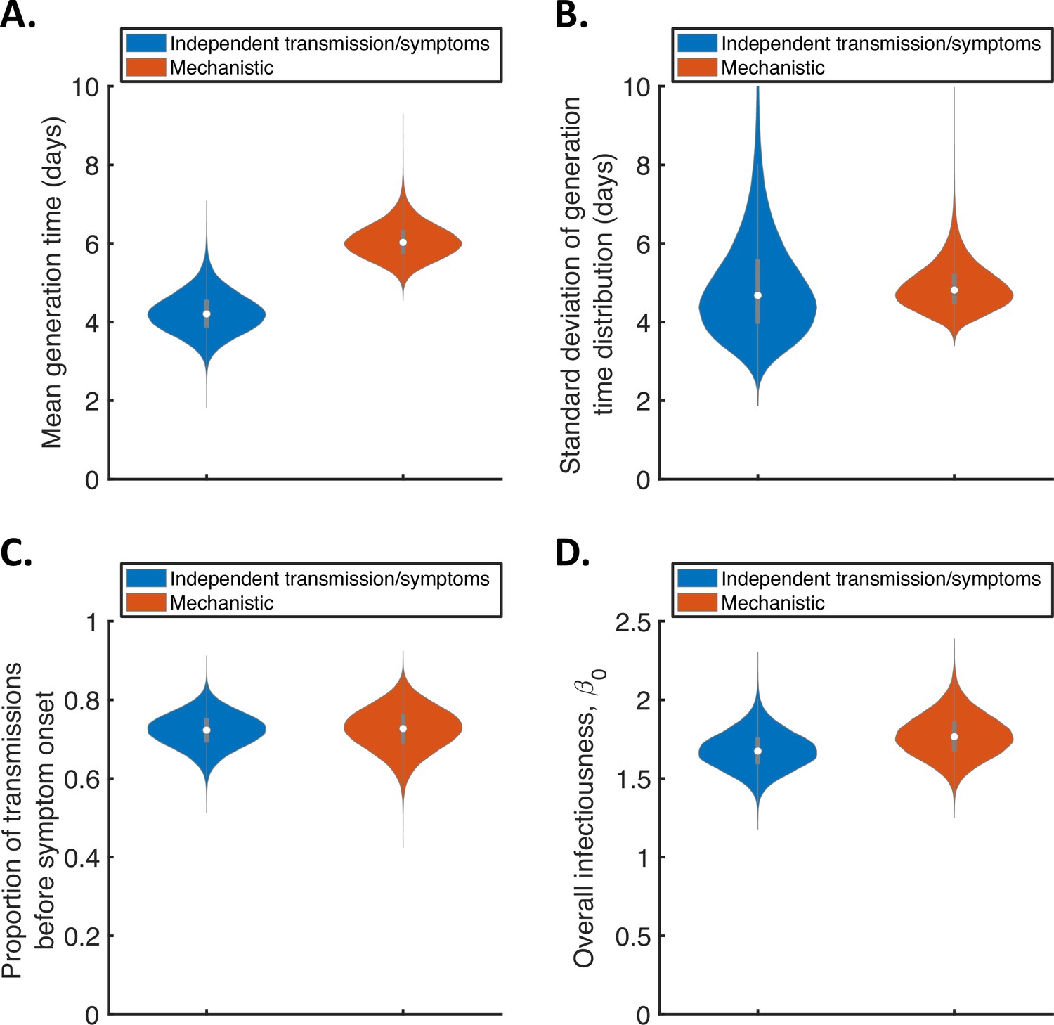
Comparison of posterior predictions.
Violin plots indicating posterior distributions of the mean (A) and standard deviation (B) of the generation time distribution, proportion of transmissions occurring prior to symptom onset (among infectors who develop symptoms; C), and overall infectiousness parameter, (describing the expected number of household transmissions generated by a single infected host) in a large, otherwise entirely susceptible, household; D). We show results obtained both using a model in which infectiousness is assumed to be independent of when symptoms develop (‘independent transmission and symptoms model’, blue), and using the mechanistic model from Hart et al., 2021 in which infectiousness is explicitly linked to symptoms (‘mechanistic model’, red).
-
Figure 1—source data 1
Household transmission data.
The transmission data from 172 households used in our analyses.
- https://cdn.elifesciences.org/articles/70767/elife-70767-fig1-data1-v2.xlsx
Figure 1—figure supplement 1
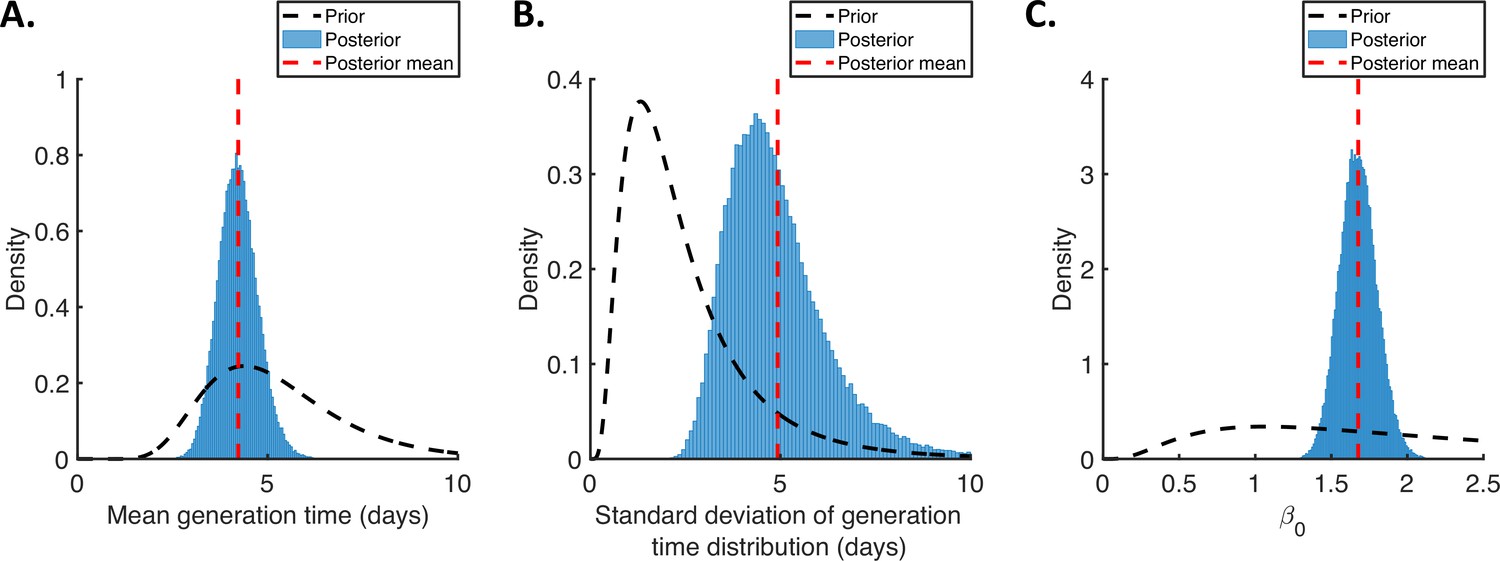
Posterior distributions of fitted parameters for the independent transmission and symptoms model.
Prior distributions (black dashed lines), posterior distributions (blue bars), and posterior means (vertical red dashed lines) of fitted parameters in the independent transmission and symptoms model. (A). Mean generation time. (B). Standard deviation of the generation time distribution. (C). Overall infectiousness, .
Figure 1—figure supplement 2
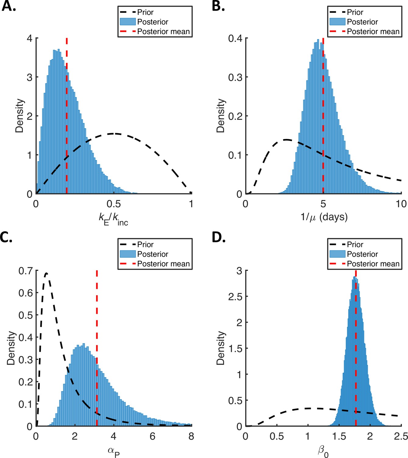
Posterior distributions of fitted parameters for the mechanistic model.
Prior distributions (black dashed lines), posterior distributions (blue bars), and posterior means (vertical red dashed lines) of fitted parameters in the mechanistic model. (A). Ratio of mean durations of the latent (E) and incubation (combined E and P) periods, . (B). Mean symptomatic infectious (I) period, . (C). Ratio of transmission rates in the presymptomatic infectious (P) and symptomatic infectious (I) stages of infection, . (D). Overall infectiousness, .
Figure 1—figure supplement 3
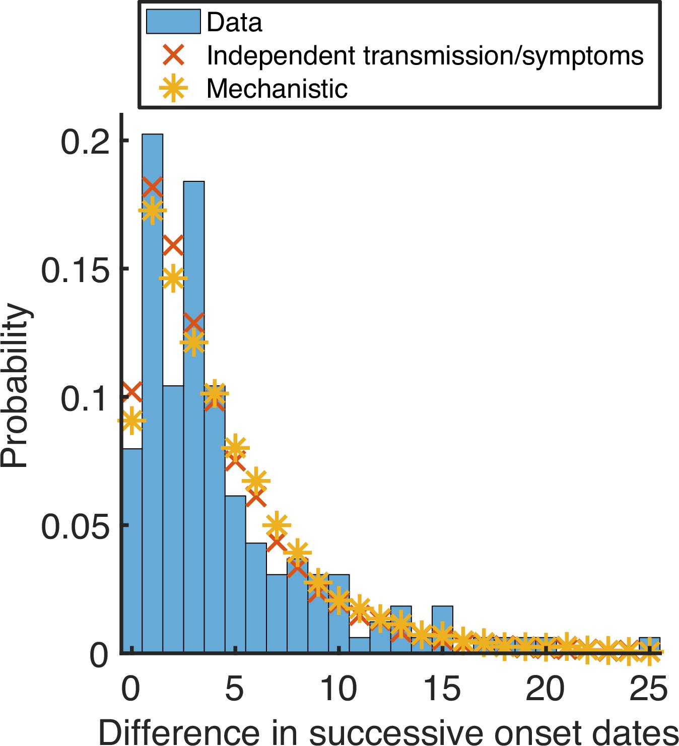
Observed and model-predicted distributions of intervals between successive household symptom onset dates.
Using posterior mean parameter estimates, we predicted the distribution of the difference in successive symptom onset dates within households (this differs from the serial interval because an infected individual may not have been infected by the previous household member to develop symptoms) under the fitted independent transmission and symptoms model (red crosses) and mechanistic model (yellow stars). These distributions were compared to the UK household data (blue bars). The distributions for the fitted models were obtained by generating synthetic data from 16,700 households using the same distribution of household sizes as in the UK data.
Figure 1—figure supplement 4
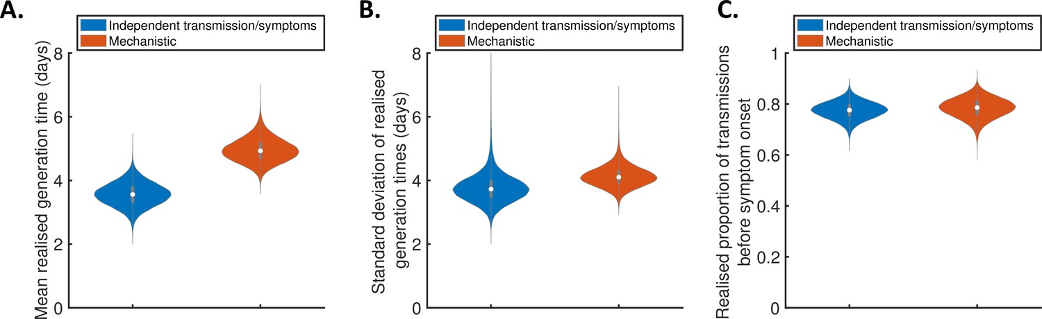
Generation times within study households.
Violin plots indicating posterior distributions of the mean (A) and standard deviation (B) of realised generation times in the study households, and the realised proportion of transmissions occurring prior to symptom onset (C), for the independent transmission and symptoms model (blue) and mechanistic model (red).
Figure 1—figure supplement 5
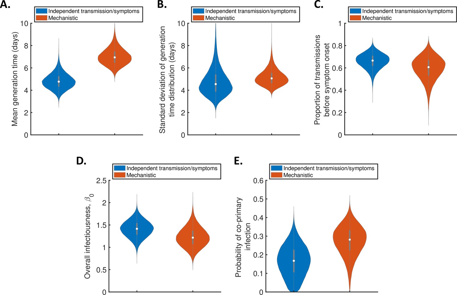
Estimates of the generation time accounting for the possibility of co-primary cases.
Violin plots indicating posterior distributions of the mean (A) and standard deviation (B) of the generation time distribution, proportion of transmissions occurring prior to symptom onset (among infectors who develop symptoms; C), overall infectiousness parameter, (D), and probability of co-primary infection (E), for the independent transmission and symptoms model (blue) and mechanistic model (red), when the possibility of co-primary cases was included in our approach (see the Appendix).
Figure 1—figure supplement 6
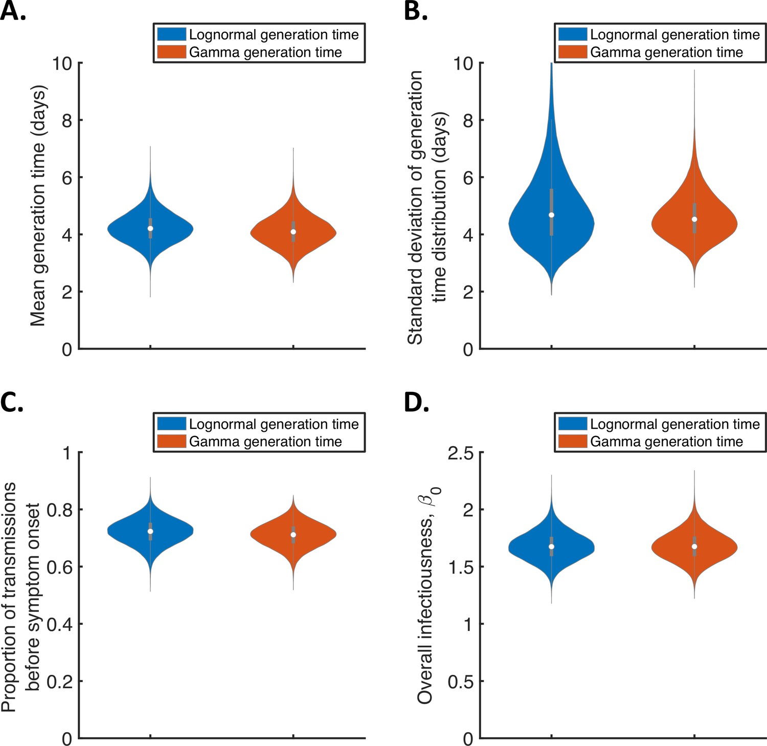
Sensitivity of the results to the functional form of the generation time distribution for the independent transmission and symptoms model.
Violin plots indicating posterior distributions of the mean (A) and standard deviation (B) of the generation time distribution, proportion of transmissions occurring prior to symptom onset (among infectors who develop symptoms; C), and overall infectiousness parameter, (D), for the independent transmission and symptoms model, when the generation time was assumed to follow either a lognormal (blue, as in Figure 1) or a gamma (red) distribution, and the incubation period distribution followed a lognormal distribution (as in Figure 1).
Figure 1—figure supplement 7
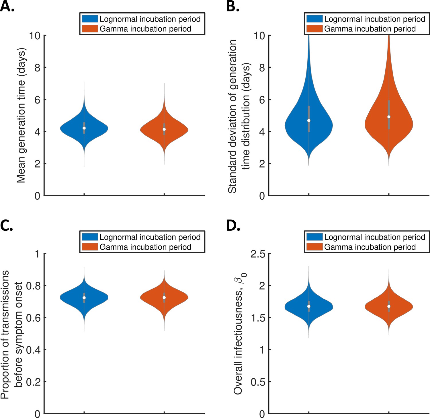
Sensitivity of the results to the functional form of the incubation period distribution for the independent transmission and symptoms model.
Violin plots indicating posterior distributions of the mean (A) and standard deviation (B) of the generation time distribution, proportion of transmissions occurring prior to symptom onset (among infectors who develop symptoms; C), and overall infectiousness parameter, (D), for the independent transmission and symptoms model, when the incubation period was assumed to follow either a lognormal distribution (blue, as in Figure 1) or a gamma distribution with the same mean and standard deviation (red), and the generation time followed a lognormal distribution (as in Figure 1).
Figure 1—figure supplement 8
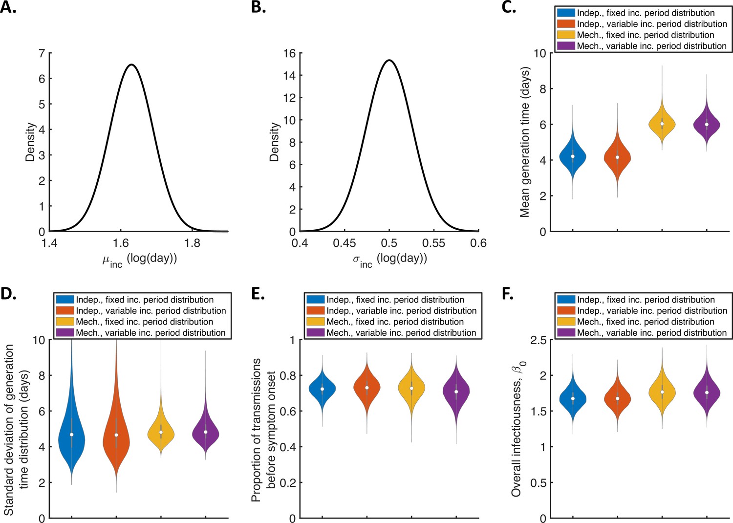
Sensitivity of the results to the incubation period distribution.
(A-B). Uncertainty in the incubation period distribution was accounted for by updating the parameters, and , of a lognormal incubation period distribution (these parameters represent the mean and standard deviation of the natural logarithm of the incubation period, respectively) alongside unknown model parameters during the MCMC procedure. Independent normal prior distributions (truncated at zero) consistent with the 95% confidence intervals obtained by McAloon et al., 2020 were assumed for (prior mean 1.63 log(day), standard deviation 0.061, 95% CrI 1.51–1.75; panel A) and (prior mean 0.5 log(day), standard deviation 0.026, 95% CrI 0.45–0.55; panel B). This incubation period was used directly when evaluating the likelihood in the independent transmission and symptoms model. In the mechanistic model, we assumed a gamma distributed incubation period with the same mean and standard deviation as a lognormal distribution with parameters and . (C-F). Violin plots indicating posterior distributions of the mean (C) and standard deviation (D) of the generation time distribution, proportion of transmissions occurring prior to symptom onset (among infectors who develop symptoms; E), and overall infectiousness parameter, (F), for the independent transmission and symptoms model with either a fixed (as in Figure 1; blue) or variable (i.e. accounting for uncertainty in and as described above; red) incubation period distribution, and for the mechanistic model with a fixed (orange) or variable (purple) incubation period distribution.
Figure 1—figure supplement 9
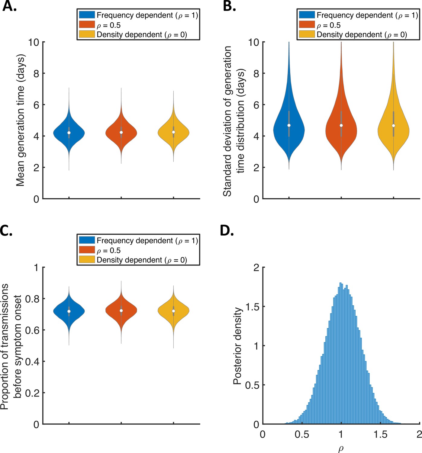
Sensitivity of the results to the dependency of transmission on the household size.
(A-C). Violin plots indicating the posterior distributions of the mean (A) and standard deviation (B) of the generation time distribution, and proportion of transmissions occurring prior to symptom onset (among infectors who develop symptoms; C), for the independent transmission and symptoms model under different assumptions about the dependency of transmission on the household size. In these panels, infectiousness is assumed to scale with , where is the household size, for (frequency-dependent transmission, blue), (red), and (density-dependent transmission, orange). (D) Posterior distribution of the dependency, , when it was fitted to the data (alongside other model parameters), assuming a uniform prior for .
Figure 1—figure supplement 10
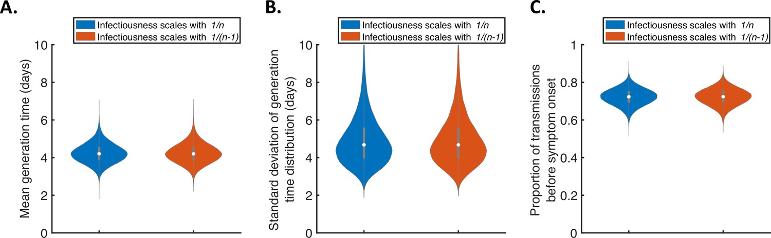
Further sensitivity of the results to the dependency of transmission on the household size.
Violin plots indicating the posterior distributions of the mean (A) and standard deviation (B) of the generation time distribution, and proportion of transmissions occurring prior to symptom onset (among infectors who develop symptoms; C), for the independent transmission and symptoms model under different assumptions about the dependency of transmission on the household size. In these panels, infectiousness is assumed to scale with either (blue) or (red).
Figure 1—figure supplement 11
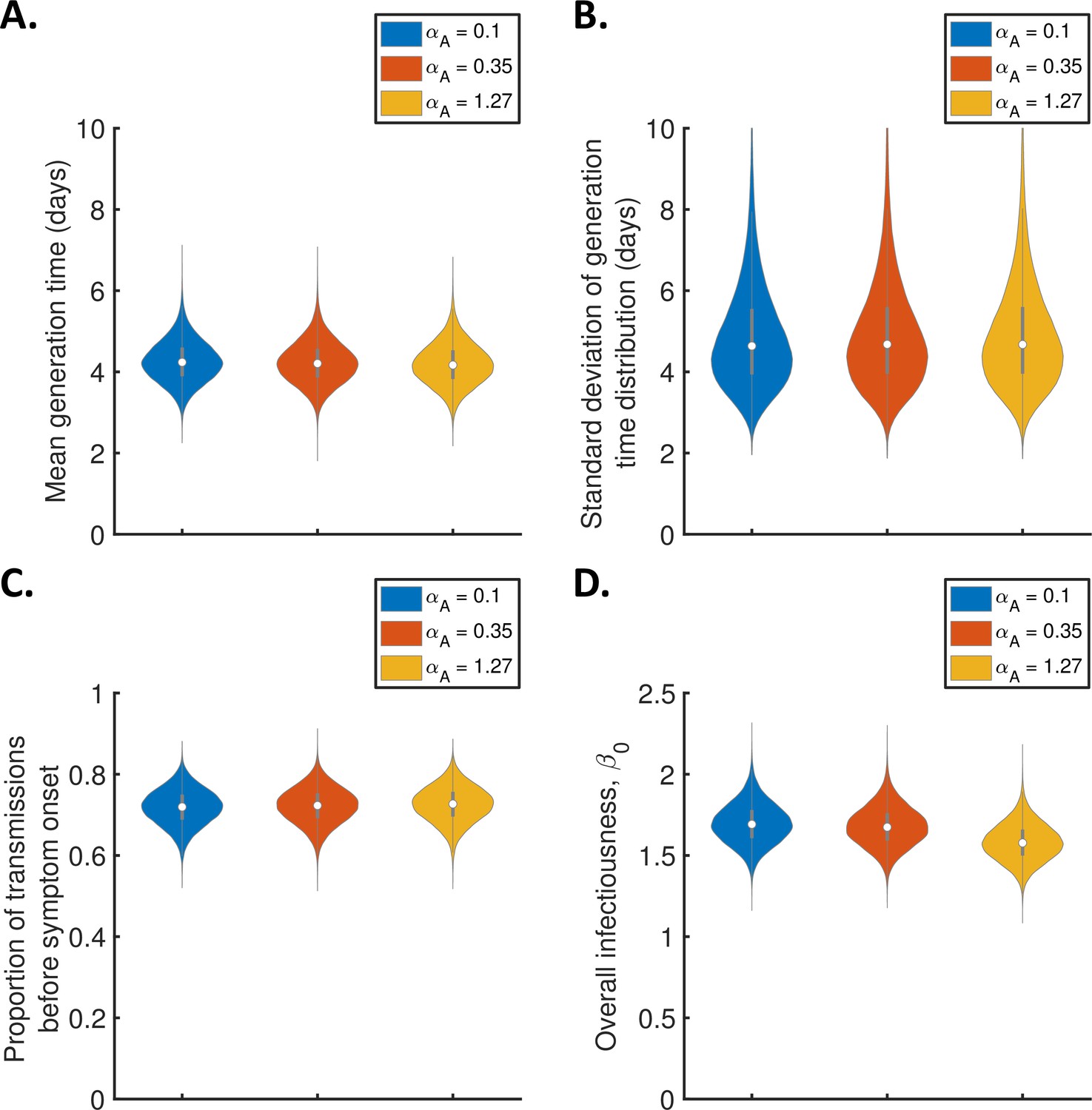
Sensitivity of the results to the relative infectiousness of entirely asymptomatic infected hosts.
Violin plots indicating posterior distributions of the mean (A) and standard deviation (B) of the generation time distribution, proportion of transmissions occurring prior to symptom onset (among infectors who develop symptoms; C), and overall infectiousness parameter, (D), for the independent transmission and symptoms model, when the relative infectiousness of asymptomatic hosts (compared to hosts who develop symptoms, at the same time since infection) was assumed to be (blue), (red), and (orange).
Figure 1—figure supplement 12
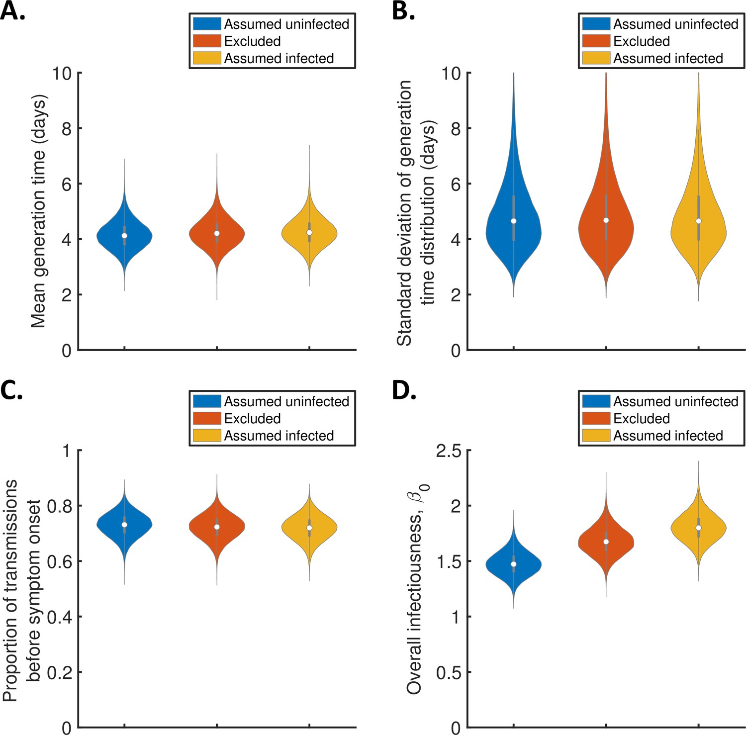
Sensitivity of the results to the exclusion of household members of unknown infection status.
(A-C). Violin plots indicating the posterior distributions of the mean (A) and standard deviation (B) of the generation time distribution, proportion of transmissions occurring prior to symptom onset (among infectors who develop symptoms; C), and overall infectiousness parameter, (D), for the independent transmission and symptoms model, when individuals of unknown infection status were assumed all uninfected (blue), excluded (red), or assumed all infected (orange).
Figure 2
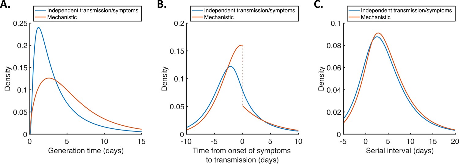
Generation time, TOST and serial interval distributions.
Inferred generation time (A), TOST (B) and serial interval (C) distributions for the two models, obtained using point estimate (posterior mean) parameters. The means and standard deviations of these distributions are given in Appendix 1—table 4. Similarly to Hart et al., 2021, the discontinuity in the red curve in (B) occurs because different transmission rates were fitted for infectors in the presymptomatic infectious (P) and symptomatic infectious (I) stages of infection. The reduction in transmission following symptom onset can be attributed to changes in behaviour in response to symptoms (Manfredi and D’Onofrio, 2013).
Figure 3 with 6 supplements
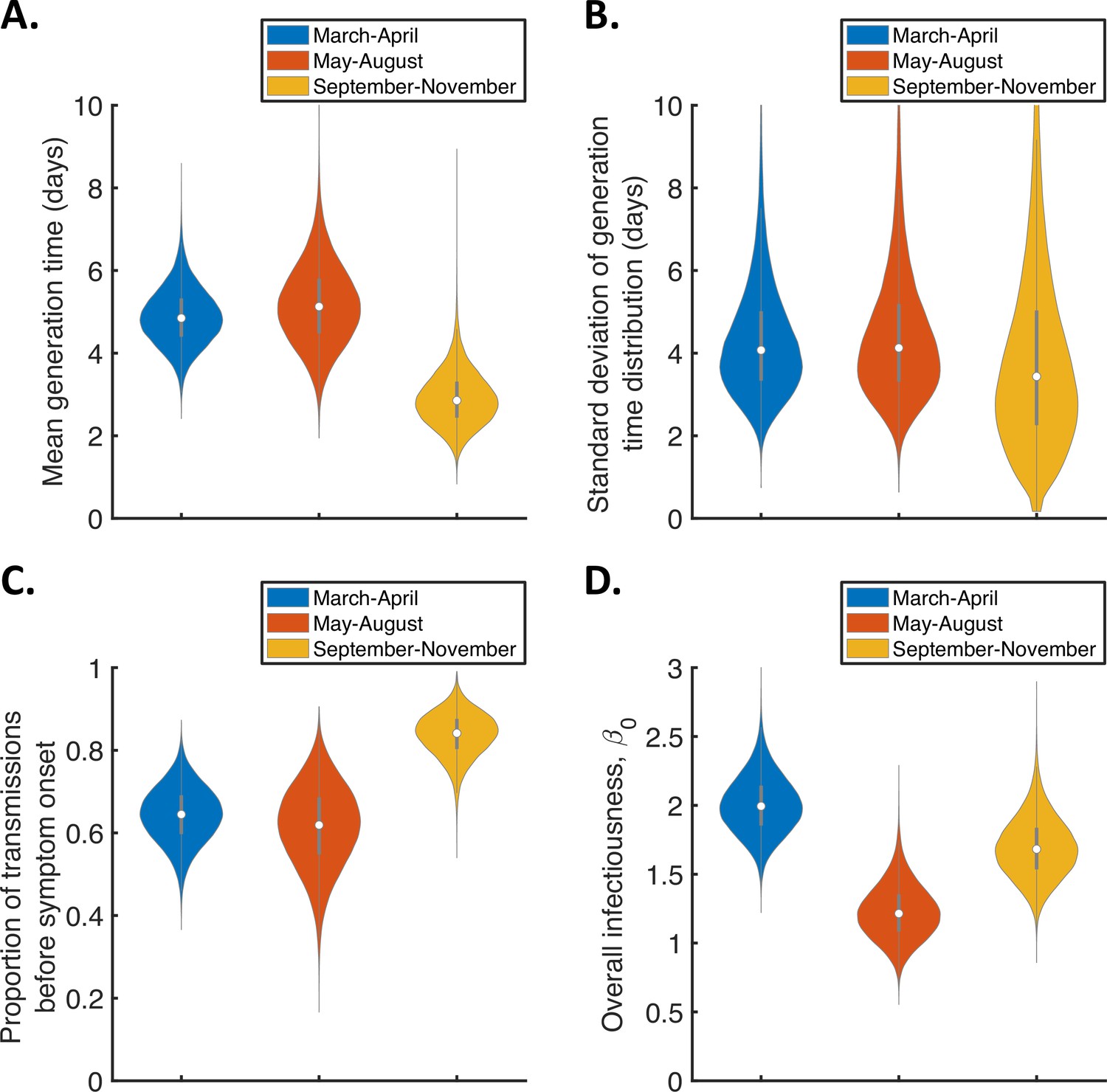
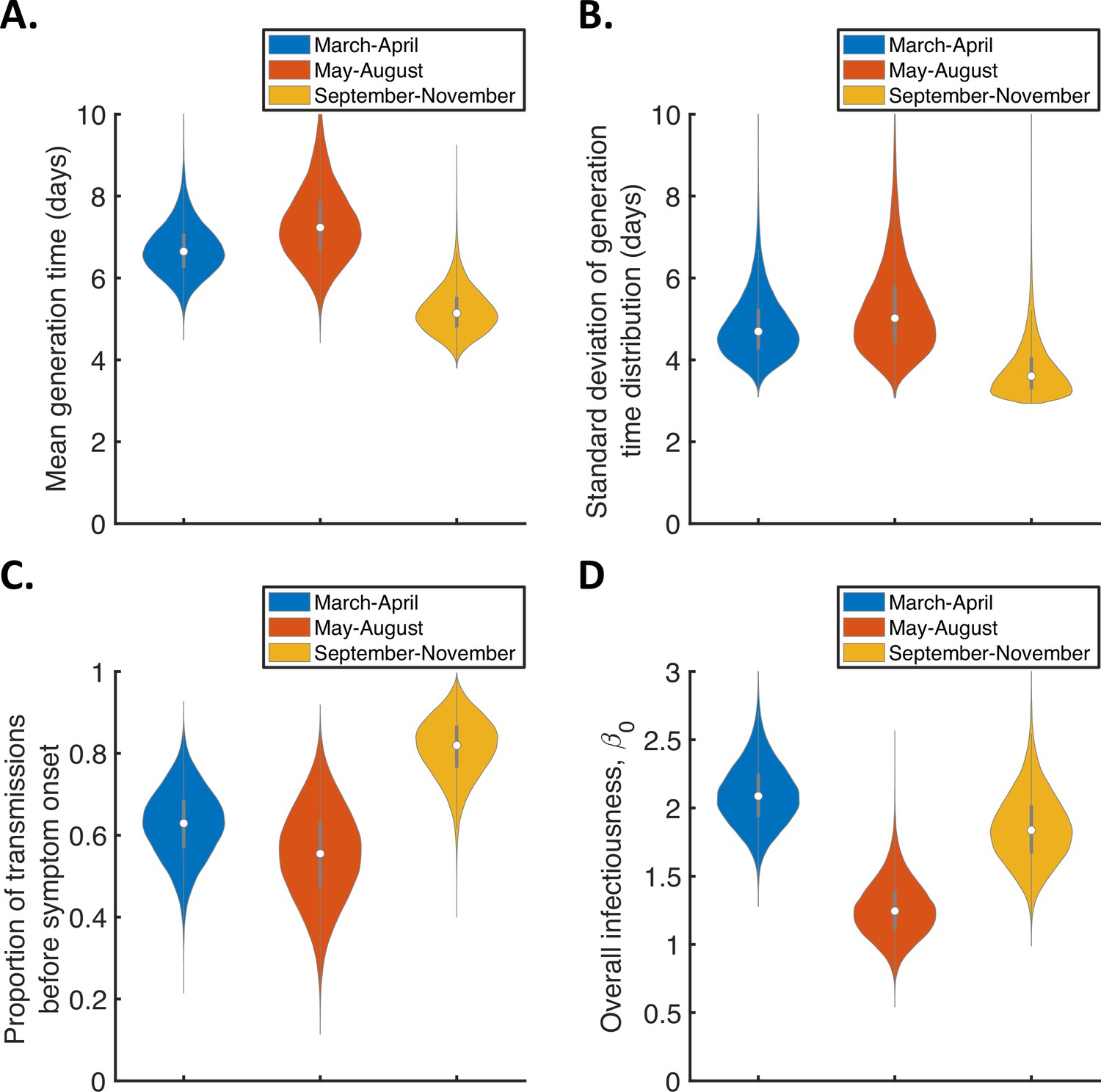
Temporal changes in the generation time.
Violin plots indicating posterior distributions of the mean (A) and standard deviation (B) of the generation time distribution, proportion of transmissions occurring prior to symptom onset (among infectors who develop symptoms; C), and overall infectiousness parameter, (D), for the independent transmission and symptoms model fitted to data from March-April (blue), May-August (red), or September-November 2020 (orange).
Figure 3—figure supplement 1
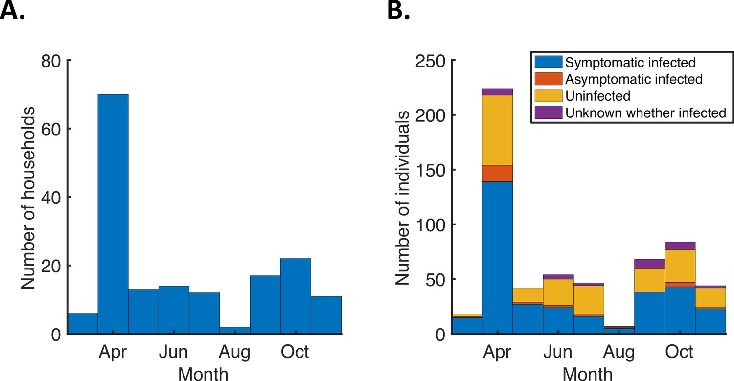
Number of study households and household members by recruitment month.
(A). Bars indicating the number of households recruited each month into the study from which we obtained the household transmission data used in our analyses, from March to November 2020 (excluding five households that were excluded from our analyses as described in Methods). (B). Stacked bars indicating the total number of individuals within the households recruited each month, distinguishing between those who were infected and developed symptoms (blue), those who were infected but never developed symptoms (red), those who remained uninfected (yellow), and those for whom it was unknown whether or not they were infected (purple).
Figure 3—figure supplement 2
Temporal changes in the generation time for the mechanistic model.
Violin plots indicating posterior distributions of the mean (A) and standard deviation (B) of the generation time distribution, proportion of transmissions occurring prior to symptom onset (among infectors who develop symptoms; C), and overall infectiousness parameter, (D), for the mechanistic model fitted to data from March-April (blue), May-August (red), or September-November 2020 (orange).
Figure 3—figure supplement 3
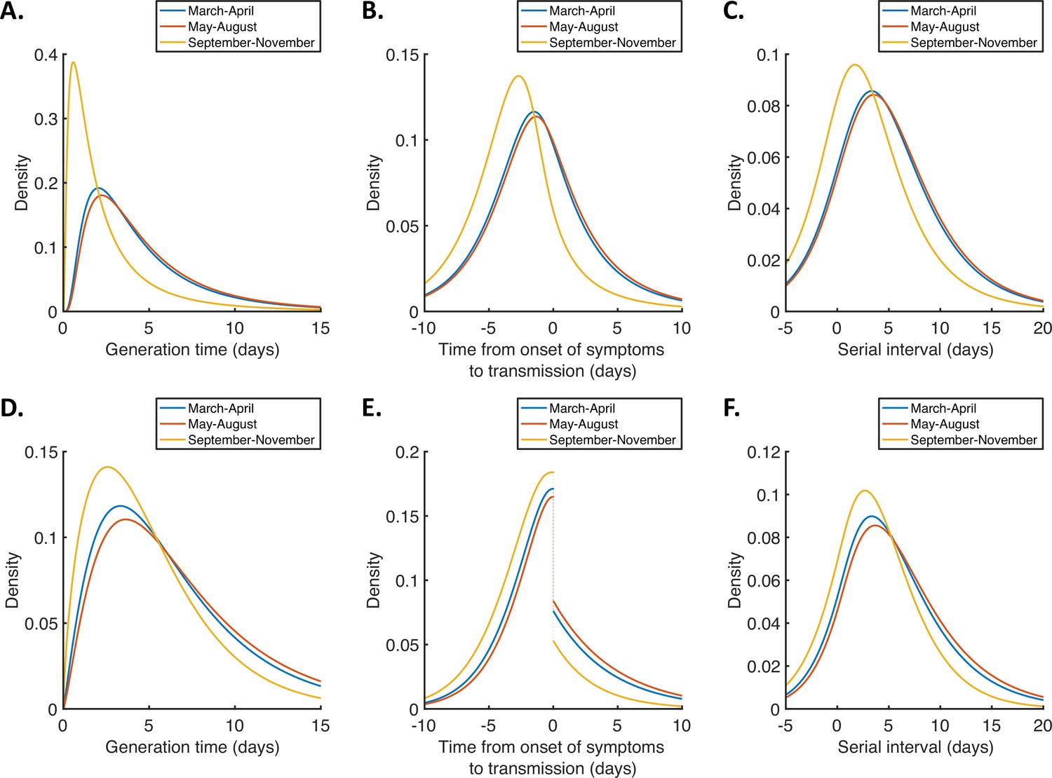
Temporal changes in the generation time, TOST and serial interval distributions.
(A-C). Inferred generation time (A), TOST (B) and serial interval (C) distributions, obtained using point estimate (posterior mean) parameters for the independent transmission and symptoms model fitted to data from March-April (blue), May-August (red), or September-November 2020 (orange). (D-F). Equivalent panels to (A-C) for the mechanistic model.
Figure 3—figure supplement 4
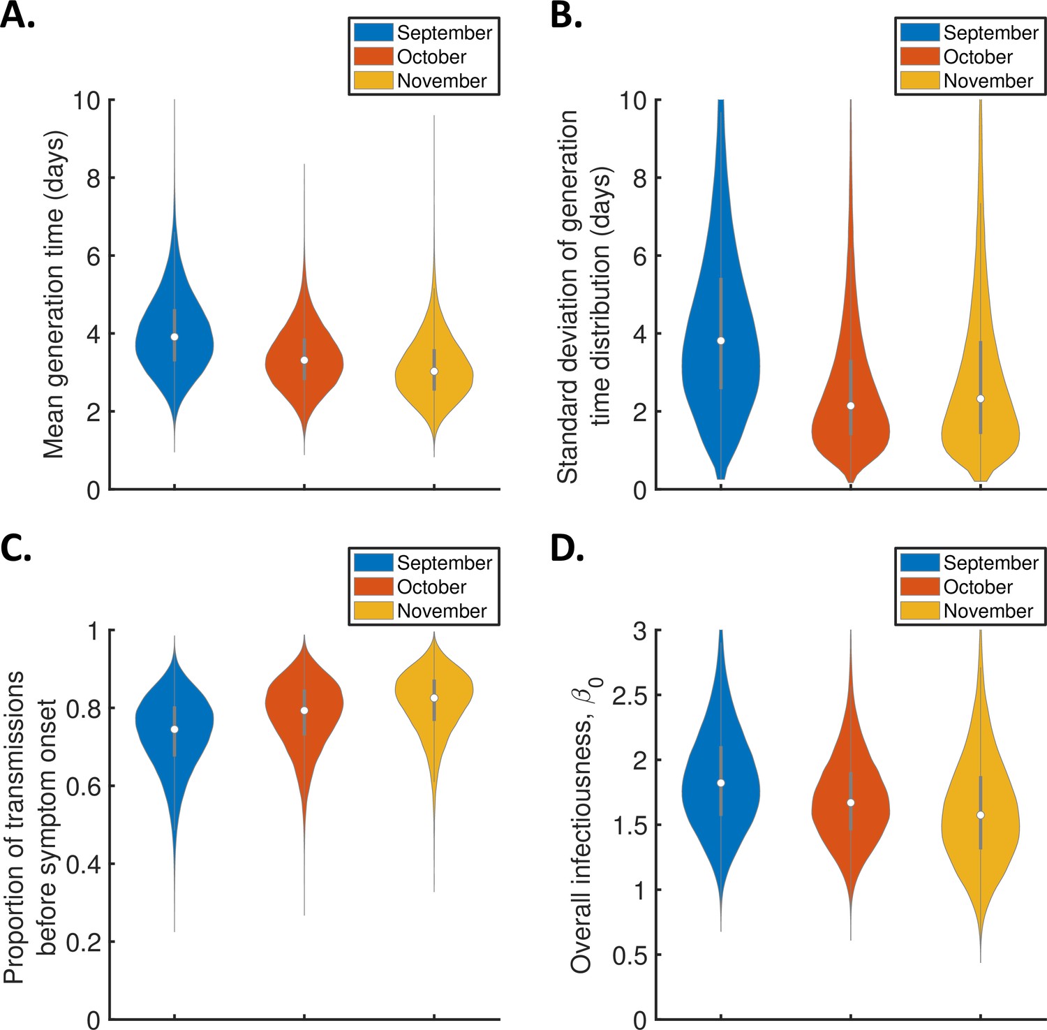
Monthly changes in the generation time from September-November 2020 for the independent transmission and symptoms model.
Violin plots indicating posterior distributions of the mean (A) and standard deviation (B) of the generation time distribution, proportion of transmissions occurring prior to symptom onset (among infectors who develop symptoms; C), and overall infectiousness parameter, (D), for the independent transmission and symptoms model fitted to data from September (blue), October (red), or November 2020 (orange).
Figure 3—figure supplement 5
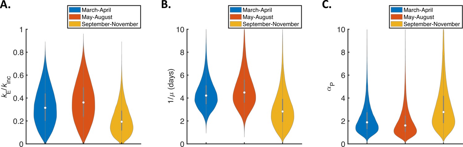
Temporal changes in fitted parameters for the mechanistic model.
Violin plots indicating posterior distributions of estimated model parameters for the mechanistic model fitted to data from March-April (blue), May-August (red), or September-November 2020 (orange). (A). Ratio of mean durations of the latent (E) and incubation (combined E and P) periods, . (B) Mean symptomatic infectious (I) period, . (C). Ratio of transmission rates in the presymptomatic infectious (P) and symptomatic infectious (I) stages of infection, . Corresponding estimates of the overall infectiousness parameter, (the other fitted model parameter) are shown in Figure 3—figure supplement 2D.
Figure 3—figure supplement 6
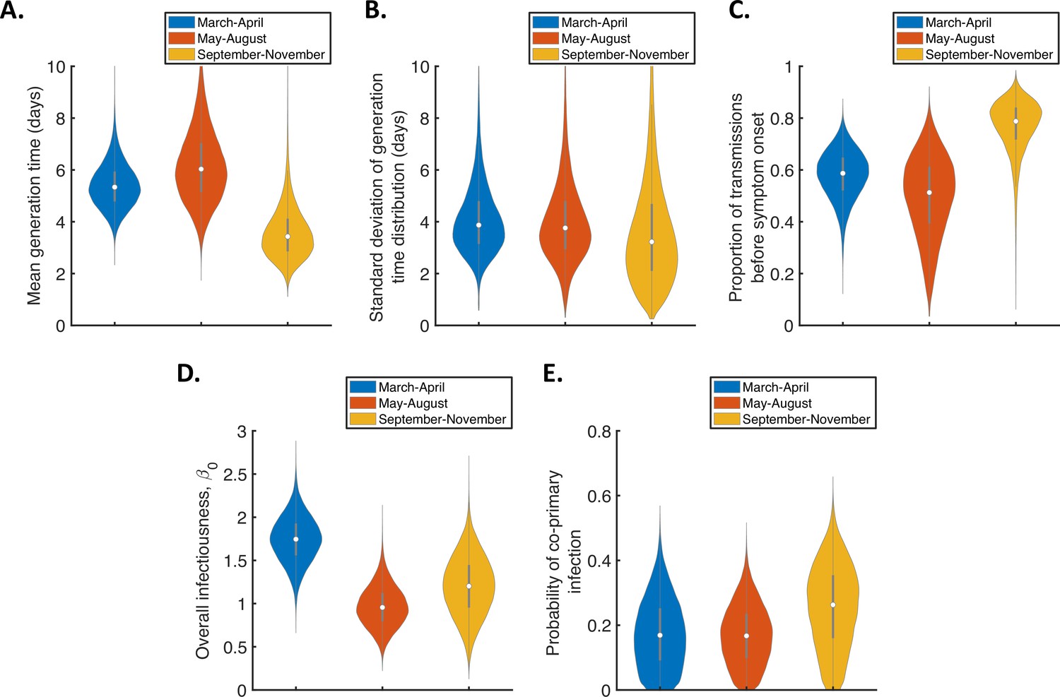
Temporal changes in the generation time for the independent transmission and symptoms model, accounting for the possibility of co-primary cases.
Violin plots indicating posterior distributions of the mean (A) and standard deviation (B) of the generation time distribution, proportion of transmissions occurring prior to symptom onset (among infectors who develop symptoms; C), overall infectiousness parameter, (D), and probability of co-primary infection (E), for the independent transmission and symptoms model fitted to data from March-April (blue), May-August (red), or September-November 2020 (orange), when the possibility of co-primary cases was included in our approach (see the Appendix).
Tables
Table 1
Previous SARS-CoV-2 generation time estimates.
Estimates of the mean and standard deviation of the generation time distribution, obtained under the assumption of independent transmission and symptoms. 95% credible intervals are shown in brackets where available.
| Study | Location | Time period | Mean generation time (days) | Standard deviation of generation time distribution (days) |
|---|---|---|---|---|
| Ferretti et al., 2020b | Various | December 2019-February 2020 | 5.0 | 1.9 |
| Ganyani et al., 2020 | Singapore | January-February 2020 | 5.20 (3.78–6.78) | 1.72 (0.91–3.93) |
| Ganyani et al., 2020 | China | January-February 2020 | 3.95 (3.01–4.91) | 1.51 (0.74–2.97) |
| Hart et al., 2021 | Various | December 2019-March 2020 | 5.57 (5.08–6.09) | 2.32 (1.83–2.91) |
| Ferretti et al., 2020a | Various | December 2019-March 2020 | 5.5 | 1.8 |
| Challen et al., 2021 | UK | January-March 2020 | 4.8 (4.3–5.41) | 1.7 (1.0–2.6) |
Appendix 1—table 1
Assumed (not fitted) parameter values used for the two models that we considered.
| Parameter | Model | Interpretation | Value | Justification |
|---|---|---|---|---|
| Both | Relative infectiousness of entirely asymptomatic hosts | 0.35 | Taken from Buitrago-Garcia et al., 2020 (other values considered in sensitivity analyses) | |
| Mean of natural logarithm of the incubation period | Independent transmission and symptoms | Parameter of lognormal incubation period distribution | 1.63 log(day) | Taken from McAloon et al., 2020 (uncertainty in this value considered in sensitivity analyses) |
| Standard deviation of natural logarithm of the incubation period | Independent transmission and symptoms | Parameter of lognormal incubation period distribution | 0.50 log(day) | Taken from McAloon et al., 2020 (uncertainty in this value considered in sensitivity analyses) |
| Mechanistic | Shape parameter of gamma incubation period distribution | 3.5 | Consistent with mean and standard deviation from McAloon et al., 2020 | |
| Mechanistic | Mean incubation period | 5.8 days | Consistent with mean and standard deviation from McAloon et al., 2020 | |
| Mechanistic | Shape parameter of (gamma) symptomatic infectious period distribution | 1 | Assumed |
Appendix 1—table 2
Fitted parameters in the independent transmission and symptoms model, the prior distributions used, and the posterior means and 95% credible intervals obtained.
| Parameter | Prior | Posterior mean (95% CrI) |
|---|---|---|
| Mean generation time | Lognormal(1.6,0.35)[prior median 5.0 days, 95% CrI 2.5–9.8 days] | 4.2 days(3.3–5.3 days) |
| Standard deviation of generation time distribution | Lognormal(0.7,0.65)[prior median 2.0 days, 95% CrI 0.6–7.2 days] | 4.9 days(3.0–8.3 days) |
| Overall infectiousness parameter, | Lognormal(0.7,0.8)[prior median 2.0, 95% CrI 0.4–9.7] | 1.7(1.4–1.9) |
Appendix 1—table 3
Fitted parameters in the mechanistic model, the prior distributions used, and the posterior means and 95% credible intervals obtained.
| Parameter | Prior | Posterior mean (95% CrI) |
|---|---|---|
| Ratio of mean durations of the latent (E) and incubation (combined E and P) periods, | Beta(2.1,2.1)[prior median 0.5, 95% CrI 0.1–0.9] | 0.2(0.03–0.5) |
| Mean symptomatic infectious (I) period, | Lognormal(1.6,0.8)[prior median 5.0 days, 95% CrI 1.0–23.8 days] | 5.0 days(3.2–7.5 days) |
| Ratio of transmission rates in the P and I stages, | Lognormal(0,0.8)[prior median 1.0, 95% CrI 0.2–4.8] | 3.1(1.2–6.9) |
| Overall infectiousness parameter, | Lognormal(0.7,0.8)[prior median 2.0, 95% CrI 0.4–9.7] | 1.8(1.5–2.1) |
Appendix 1—table 4
The means and standard deviations of the generation time, TOST and serial interval distributions shown in Figure 2.
Other than the generation time distribution for the independent transmission and symptoms model (which is lognormal with the specified mean and standard deviation), none of the remaining distributions take a simple parametric form.
| Model | Distribution | Mean | Standard deviation |
|---|---|---|---|
| Independent transmission and symptoms | Generation time | 4.2 days | 4.9 days |
| TOST | −1.6 days | 5.8 days | |
| Serial interval | 4.2 days | 6.6 days | |
| Mechanistic | Generation time | 5.9 days | 4.8 days |
| TOST | −1.1 days | 4.9 days | |
| Serial interval | 4.7 days | 5.8 days |
Additional files
Download links
A two-part list of links to download the article, or parts of the article, in various formats.
Downloads (link to download the article as PDF)
Open citations (links to open the citations from this article in various online reference manager services)
Cite this article (links to download the citations from this article in formats compatible with various reference manager tools)
Inference of the SARS-CoV-2 generation time using UK household data
eLife 11:e70767.
https://doi.org/10.7554/eLife.70767


