Research Advance

Epidemiology and Global Health

Inference of the SARS-CoV-2 generation time using UK household data

Mathematical Institute, University of Oxford, United Kingdom
Centre for the Mathematical Modelling of Infectious Diseases, London School of Hygiene and Tropical Medicine, United Kingdom
Department of Infectious Disease Epidemiology, London School of Hygiene and Tropical Medicine, United Kingdom
Immunisation and Countermeasures Division, UK Health Security Agency, United Kingdom
Data and Analytical Sciences, UK Health Security Agency, United Kingdom
Mathematics Institute, University of Warwick, United Kingdom
Zeeman Institute for Systems Biology and Infectious Disease Epidemiology Research, University of Warwick, United Kingdom

Feb 9, 2022

https://doi.org/10.7554/eLife.70767

Open access
Copyright information

Version of Record

Accepted for publication after peer review and revision.

Download
Cite
Share
CommentOpen annotations (there are currently 0 annotations on this page).

Version of Record published: March 30, 2022 (This version)
Accepted Manuscript published: February 9, 2022 (Go to version)
Accepted: February 7, 2022
Preprint posted: May 30, 2021 (Go to version)
Received: May 29, 2021

1. Builds upon
High infectiousness immediately before COVID-19 symptom onset highlights the importance of continued contact tracing

William S Hart, Philip K Maini, Robin N Thompson

Short Report Jun 11, 2021
Further reading

Abstract
Editor's evaluation
Introduction
Results
Discussion
Methods
Appendix 1
Data availability
References
Decision letter
Author response
Article and author information
Metrics

Abstract

The distribution of the generation time (the interval between individuals becoming infected and transmitting the virus) characterises changes in the transmission risk during SARS-CoV-2 infections. Inferring the generation time distribution is essential to plan and assess public health measures. We previously developed a mechanistic approach for estimating the generation time, which provided an improved fit to data from the early months of the COVID-19 pandemic (December 2019-March 2020) compared to existing models (Hart et al., 2021). However, few estimates of the generation time exist based on data from later in the pandemic. Here, using data from a household study conducted from March to November 2020 in the UK, we provide updated estimates of the generation time. We considered both a commonly used approach in which the transmission risk is assumed to be independent of when symptoms develop, and our mechanistic model in which transmission and symptoms are linked explicitly. Assuming independent transmission and symptoms, we estimated a mean generation time (4.2 days, 95% credible interval 3.3–5.3 days) similar to previous estimates from other countries, but with a higher standard deviation (4.9 days, 3.0–8.3 days). Using our mechanistic approach, we estimated a longer mean generation time (5.9 days, 5.2–7.0 days) and a similar standard deviation (4.8 days, 4.0–6.3 days). As well as estimating the generation time using data from the entire study period, we also considered whether the generation time varied temporally. Both models suggest a shorter mean generation time in September-November 2020 compared to earlier months. Since the SARS-CoV-2 generation time appears to be changing, further data collection and analysis is necessary to continue to monitor ongoing transmission and inform future public health policy decisions.

Editor's evaluation

This paper is a timely update to the authors previous work and will be of interest to those working on public health responses and the mathematical modelling of infectious diseases. In this work the authors infer the generation interval of SARS–CoV–2 which can allow for the assessment of public health measures. The derivation of the likelihood function is also of interest to mathematical modellers as it allows for the inference of the generation interval from data sets where susceptible depletion may dominate infection dynamics.

https://doi.org/10.7554/eLife.70767.sa0

Introduction

The generation time (or generation interval) of a SARS-CoV-2 infector-infectee pair is defined as the period of time between the infector and infectee each becoming infected (Anderson and May, 1992; Diekmann and Heesterbeek, 2000; Griffin et al., 2020; Svensson, 2007; Wallinga and Lipsitch, 2007). The generation time distribution of many infector-infectee pairs characterises the temporal profile of the transmission risk of an infected host (averaged over all hosts and normalised so that it represents a valid probability distribution; Fraser, 2007). Inferring the generation time distribution of SARS-CoV-2 is important in order to predict the effects of non-pharmaceutical interventions such as contact tracing and quarantine (Ashcroft et al., 2021; Ferretti et al., 2020b; Hart et al., 2021). In addition, the generation time distribution is widely used in epidemiological models for estimating the time-dependent reproduction number from case notification data (Abbott et al., 2020; Fraser, 2007; Gostic et al., 2020; Thompson et al., 2020) and is crucial for understanding the relationship between the reproduction number and the epidemic growth rate (Fraser, 2007; Parag et al., 2021; Park et al., 2020a; Wallinga and Lipsitch, 2007).

The SARS-CoV-2 generation time distribution has previously been estimated using data from known infector-infectee transmission pairs (Ferretti et al., 2020a; Ferretti et al., 2020b; Hart et al., 2021) or entire clusters of cases (Ganyani et al., 2020; Hu et al., 2021; Sun et al., 2021). These studies involved data (Cheng et al., 2020; Ferretti et al., 2020b; Ganyani et al., 2020; He et al., 2020; Xia et al., 2020; Zhang et al., 2020) collected between December 2019 and April 2020, almost entirely from countries in East and Southeast Asia (with the exception of four transmission pairs from Germany and four from Italy in Ferretti et al., 2020b). Evidence from January and February 2020 in China suggested a temporal reduction in the mean generation time due to non-pharmaceutical interventions (Sun et al., 2021). Specifically, effective isolation of infected individuals is likely to have reduced the proportion of transmissions occurring when potential infectors were in the later stages of infection, thereby shortening the generation time (Sun et al., 2021). Similarly, two other studies found a decrease in the serial interval (the difference between symptom onset times of an infector and infectee; Ali et al., 2020) and an increase in the proportion of presymptomatic transmissions (Bushman et al., 2021) in China over the same time period, which can be attributed to symptomatic hosts being isolated increasingly quickly over time.

Despite estimation of the SARS-CoV-2 generation time in Asia early in the pandemic, relatively little is known about the generation time distribution outside Asia, and whether or not any changes have occurred in the generation time since the early months of the pandemic. At the time of writing, we are aware of only one previous study in which the generation time was estimated using data from the UK (Challen et al., 2021). In that study (Challen et al., 2021), data describing symptom onset dates for 50 infector-infectee pairs, collected by Public Health England (PHE; now the UK Health Security Agency) between January and March 2020 as part of the ‘First Few Hundred’ case protocol (Boddington et al., 2021; Public Health England, 2020), were used to infer the generation time distribution. However, since these transmission pairs mostly consisted of international travellers and their household contacts, the authors concluded that their estimates of the generation time may have been biased downwards due to enhanced surveillance and isolation of these cases (Challen et al., 2021).

Here, we use data from a household study (Miller et al., 2021), conducted between March and November 2020, to estimate the SARS-CoV-2 generation time distribution in the UK under two different underlying transmission models. In the first model (the ‘independent transmission and symptoms model’), a parsimonious assumption is made that the generation time and the incubation period of the infector are independent (i.e. there is no link between the times at which infectors transmit the virus and the times at which they develop symptoms), as has often been employed in studies in which the SARS-CoV-2 generation time has been estimated (Challen et al., 2021; Ferretti et al., 2020a; Ganyani et al., 2020; Hart et al., 2021; Lehtinen et al., 2021; Table 1). In the second model (the ‘mechanistic model’), we use a mechanistic approach in which potential infectors progress through different stages of infection, first becoming infectious before developing symptoms (Hart et al., 2021). Infectiousness is therefore explicitly linked to symptoms in the mechanistic model. A feature of the mechanistic model is that individuals with longer incubation periods will (on average) be infectious for longer before developing symptoms, and so generate more transmissions, compared to those with shorter incubation periods.

By fitting separately to data from three different time intervals within the study period, we explore whether or not there was a detectable temporal change in the generation time distribution.

Table 1

Previous SARS-CoV-2 generation time estimates.

Estimates of the mean and standard deviation of the generation time distribution, obtained under the assumption of independent transmission and symptoms. 95% credible intervals are shown in brackets where available.

Study	Location	Time period	Mean generation time (days)	Standard deviation of generation time distribution (days)
Ferretti et al., 2020b	Various	December 2019-February 2020	5.0	1.9
Ganyani et al., 2020	Singapore	January-February 2020	5.20 (3.78–6.78)	1.72 (0.91–3.93)
Ganyani et al., 2020	China	January-February 2020	3.95 (3.01–4.91)	1.51 (0.74–2.97)
Hart et al., 2021	Various	December 2019-March 2020	5.57 (5.08–6.09)	2.32 (1.83–2.91)
Ferretti et al., 2020a	Various	December 2019-March 2020	5.5	1.8
Challen et al., 2021	UK	January-March 2020	4.8 (4.3–5.41)	1.7 (1.0–2.6)

Results

Inferring the generation time from UK household data

We fitted two models of infectiousness (the independent transmission and symptoms model and the mechanistic model) to data collected from 172 UK households in a study (Miller et al., 2021) conducted by PHE between March and November 2020 (Figure 1—source data 1). Each household was recruited to the study following a confirmed SARS-CoV-2 infection, and all household members were then followed to investigate whether or not they became infected (this was determined through PCR and antibody testing). If a household member was infected and developed symptoms, their symptom onset date was recorded (see Methods).

In our previous work (Hart et al., 2021), we fitted the same two models of infectiousness to data from infector-infectee transmission pairs collected in the early months of the COVID-19 pandemic. Here, we adapted the approach presented in that article (Hart et al., 2021) in order to estimate the generation time using household transmission data. Specifically, we used data augmentation MCMC, augmenting the observed data with both estimated times of infection and estimated precise times at which symptomatic infected hosts developed symptoms (within recorded symptom onset dates). This enabled us (in the likelihood function) to account for uncertainty about exactly who-infected-whom within a household by summing together likelihood contributions corresponding to infection by different possible infectors. In addition, we corrected for the regularity of household contacts to derive more widely applicable estimates of the generation time. We did this by including a factor in the likelihood to account for each infected individual avoiding infection from household contacts that occurred prior to their actual time of infection (see Methods for full details of our approach).

For the two fitted models, we calculated posterior estimates of the mean (Figure 1A) and standard deviation (Figure 1B) of the generation time distribution, in addition to the proportion of transmissions occurring prior to symptom onset (among infectors who develop symptoms; Figure 1C) and the overall infectiousness parameter, $β_{0}$ (see Methods; Figure 1D). Under the commonly used independent transmission and symptoms model, we obtained a point estimate of 4.2 days (95% credible interval (CrI) 3.3–5.3 days) for the mean generation time (Figure 1A, blue violin; we calculated point estimates for each model using the posterior means of fitted model parameters because the mode of the joint posterior distribution could not easily be calculated from the output of the MCMC procedure). This value is similar to a previous estimate obtained using data from China by Ganyani et al., 2020. It is slightly lower than estimates for Singapore obtained by Ganyani et al., 2020 and for several countries (predominantly in Asia) obtained by Ferretti et al., 2020b (Table 1), although those estimates lie within our credible interval. On the other hand, our estimated standard deviation of 4.9 days (95% CrI 3.0–8.3 days; Figure 1B, blue violin) is substantially higher than previous estimates (Table 1). Using our mechanistic model, we obtained a higher estimate for the mean generation time of 5.9 days (95% CrI 5.2–7.0 days; Figure 1A, red violin), and a similar estimate for the standard deviation (4.8 days, 95% CrI 4.0–6.3 days; Figure 1B, red violin), compared to those predicted by the independent transmission and symptoms model.

Figure 1 with 12 supplements see all

Download asset Open asset

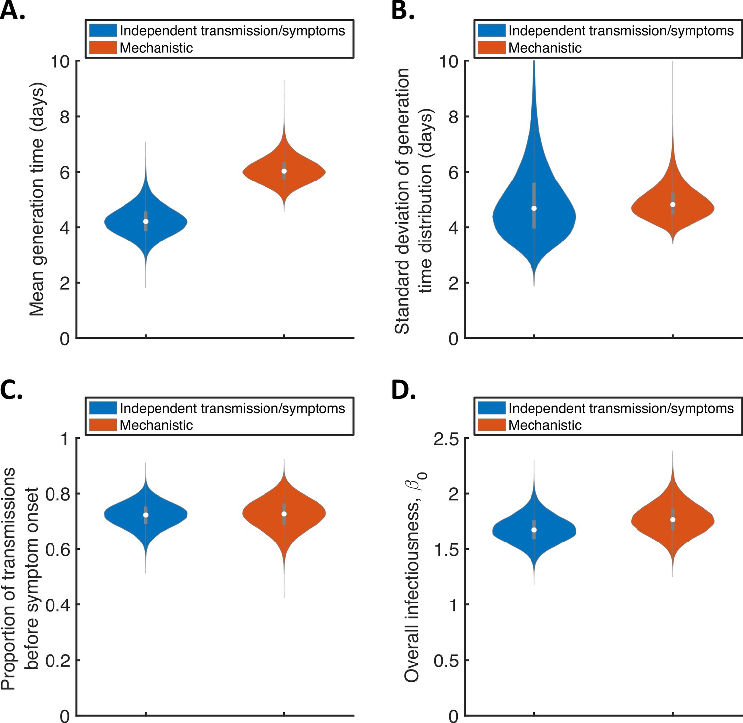
Comparison of posterior predictions.

Violin plots indicating posterior distributions of the mean (A) and standard deviation (B) of the generation time distribution, proportion of transmissions occurring prior to symptom onset (among infectors who develop symptoms; C), and overall infectiousness parameter, $β_{0}$ (describing the expected number of household transmissions generated by a single infected host) in a large, otherwise entirely susceptible, household; D). We show results obtained both using a model in which infectiousness is assumed to be independent of when symptoms develop (‘independent transmission and symptoms model’, blue), and using the mechanistic model from Hart et al., 2021 in which infectiousness is explicitly linked to symptoms (‘mechanistic model’, red).

Figure 1—source data 1 Household transmission data. The transmission data from 172 households used in our analyses.: https://cdn.elifesciences.org/articles/70767/elife-70767-fig1-data1-v2.xlsx
Download elife-70767-fig1-data1-v2.xlsx

The two models gave similar posterior distributions for the proportion of transmissions prior to symptom onset (Figure 1C). Specifically, point estimate values of model parameters led to an estimated proportion of transmissions prior to symptom onset of 0.72 (95% CrI 0.63–0.80) for the independent transmission and symptoms model, and 0.73 (95% CrI 0.61–0.83) for the mechanistic model. These estimates are higher than obtained in some previous studies in which the infectiousness profile of SARS-CoV-2 infected hosts at each time since infection and/or time since symptom onset has been estimated (Ashcroft et al., 2020; Ferretti et al., 2020a; He et al., 2020). On the other hand, our point estimates for the two models both lie within the 95% credible interval obtained for the mechanistic model in our previous work (0.53–0.77, point estimate 0.65; Hart et al., 2021). Similar or higher estimates also exist in the wider literature (Casey-Bryars et al., 2021; Ganyani et al., 2020; Tindale et al., 2020).

Posterior distributions for fitted model parameters are shown in Figure 1—figure supplement 1 and Figure 1—figure supplement 2, and point estimates and 95% credible intervals are given in Appendix 1—table 2 and Appendix 1—table 3. Since only the likelihood with respect to augmented data was calculated in the MCMC procedure, direct comparisons of the goodness of fit between the models were not readily available. However, comparing model predictions of the distribution of the interval between successive symptom onset dates in households to the analogous distribution in the data indicated that both models provided a similar fit to the data (Figure 1—figure supplement 3).

In Figure 1 (and elsewhere, unless otherwise stated), we characterise the generation time distribution assuming that a constant supply of susceptible individuals are available to infect during the course of infection. This distribution corresponds to the normalised expected infectiousness profile of an infected host at each time since infection, and is widely applicable to transmission outside of, as well as within, households. However, realised household generation times are expected to be shorter than the estimates shown in Figure 1. This is due to the depletion of susceptible household members before longer generation times can be obtained, especially in small households (Cauchemez et al., 2009; Fraser, 2007; Park et al., 2020a). As a result, we also predicted the mean and standard deviation of realised generation times within the study households (Figure 1—figure supplement 4A,B), accounting for the precise distribution of household sizes in the study. For both the independent transmission and symptoms model and the mechanistic model, the mean (point estimates 3.6 days and 4.9 days for the two models, respectively) and standard deviation (3.8 days and 4.1 days) of realised household generation times were lower than our main generation time estimates shown in Figure 1. Since household transmission typically occurs earlier in the infector’s course of infection than indicated by the estimates shown in Figure 1, we predicted a higher proportion of presymptomatic transmissions within the study households (Figure 1—figure supplement 4C) compared to the estimates in Figure 1C.

For both models, we then used point estimates of fitted model parameters to infer the distributions of the generation time (Figure 2A), the time from onset of symptoms to transmission (TOST; Figure 2B) and the serial interval (Figure 2C). The TOST distribution (which characterises the relative expected infectiousness of a host (who develops symptoms) at each time from symptom onset, as opposed to from infection [Ashcroft et al., 2020; Ferretti et al., 2020a; He et al., 2020; Lehtinen et al., 2021; Wells et al., 2021]) obtained using the mechanistic model was more concentrated around the time of symptom onset compared to that predicted assuming independent transmission and symptoms (Figure 2B), as we found in our previous work (Hart et al., 2021). In contrast, the estimated serial interval distributions were similar for the two models (Figure 2C). The means and standard deviations of the distributions shown in Figure 2 are given in Appendix 1—table 4.

Figure 2

Download asset Open asset

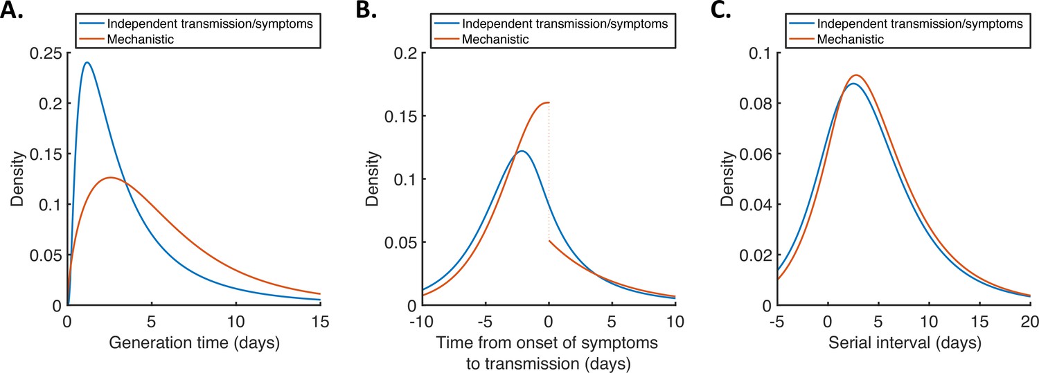
Generation time, TOST and serial interval distributions.

Inferred generation time (A), TOST (B) and serial interval (C) distributions for the two models, obtained using point estimate (posterior mean) parameters. The means and standard deviations of these distributions are given in Appendix 1—table 4. Similarly to Hart et al., 2021, the discontinuity in the red curve in (B) occurs because different transmission rates were fitted for infectors in the presymptomatic infectious (P) and symptomatic infectious (I) stages of infection. The reduction in transmission following symptom onset can be attributed to changes in behaviour in response to symptoms (Manfredi and D’Onofrio, 2013).

Temporal variation in the generation time distribution

To explore whether or not the generation time distribution changed during the study period, we separately fitted the independent transmission and symptoms model to the data from households in which the index case was recruited in (i) March-April, (ii) May-August, or (iii) September-November 2020 (Figure 3). We chose these time periods to ensure the numbers of households recruited into the study during each interval were similar (Figure 3—figure supplement 1).

Figure 3 with 6 supplements see all

Download asset Open asset

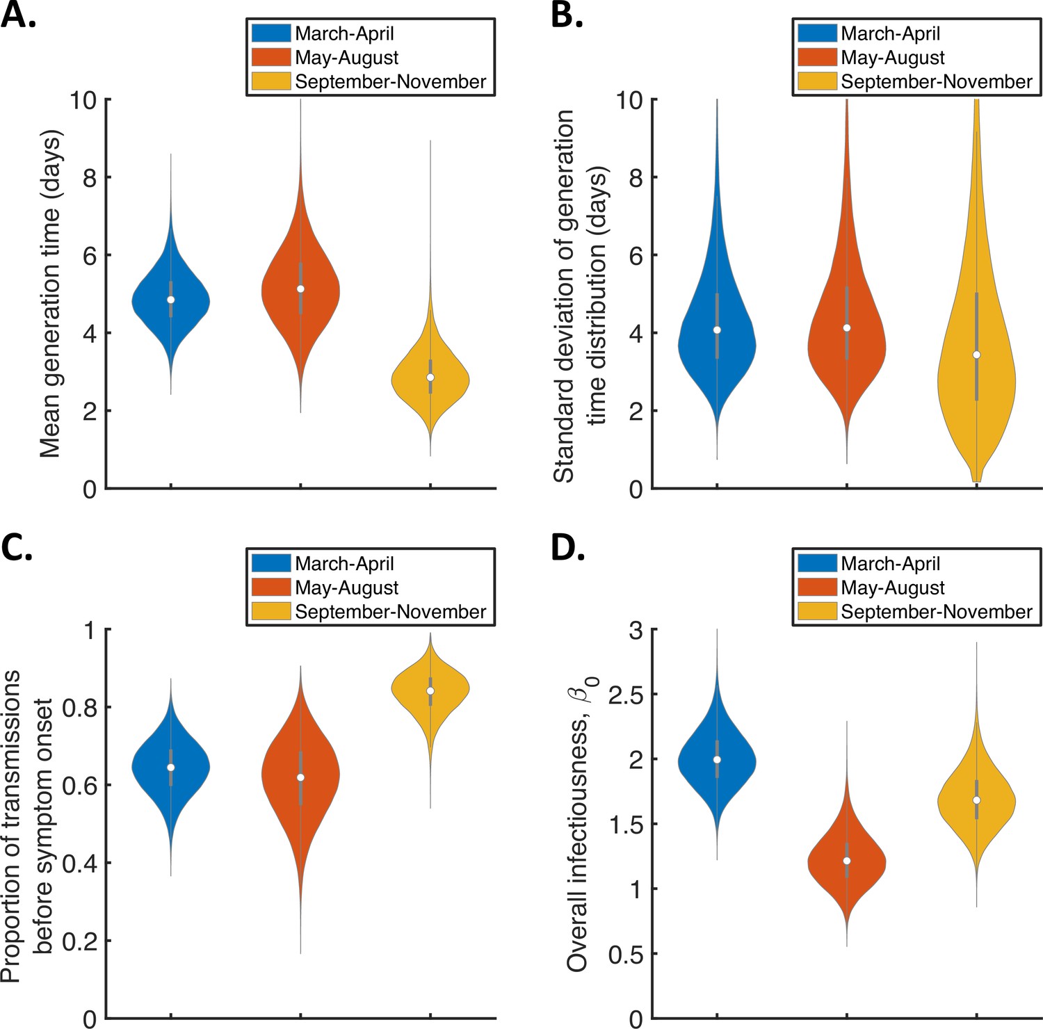
Temporal changes in the generation time.

Violin plots indicating posterior distributions of the mean (A) and standard deviation (B) of the generation time distribution, proportion of transmissions occurring prior to symptom onset (among infectors who develop symptoms; C), and overall infectiousness parameter, $β_{0}$ (D), for the independent transmission and symptoms model fitted to data from March-April (blue), May-August (red), or September-November 2020 (orange).

The results shown in Figure 3A suggest a shorter mean generation time in September-November 2020 (2.9 days, 95% CrI 1.8–4.3 days) compared to earlier months (4.9 days, 95% CrI 3.6–6.3 days, for March-April and 5.2 days, 95% CrI 3.4–7.2 days, for May-August). Comparing the posterior estimates for May-August and September-November (the red and orange violins in Figure 3A, respectively) indicated a 97% posterior probability of a shorter mean generation time in the later of these two time periods. A similar temporal reduction in the mean generation time was found when we instead fitted the mechanistic model to the data from the three time intervals (Figure 3—figure supplement 2). Estimates of the mean generation time using the mechanistic model were 6.5 days (95% CrI 5.6–8.1 days) for March-April, 7.1 days (95% CrI 5.7–9.6 days) for May-August, and 5.1 days (95% CrI 4.3–6.4 days) for September-November, with a 98% posterior probability of a shorter mean generation time in September-November than May-August. We also used point estimates of model parameters to compare the distributions of the generation time, TOST and serial interval between the time periods (Figure 3—figure supplement 3), with both models indicating that the transmission risk peaked earlier in infection for individuals infected in September-November compared to earlier months (Figure 3—figure supplement 3A,D).

Figure 3C shows posterior estimates for the proportion of transmissions occurring prior to symptom onset (among symptomatic infectors) across the three time periods for the independent transmission and symptoms model, indicating a very high proportion of presymptomatic transmissions in September-November (0.83, 95% CrI 0.72–0.93) compared to lower estimates for March-April (0.64, 95% CrI 0.51–0.77) and May-August (0.62, 95% CrI 0.41–0.79). Our results for the mechanistic model indicate a similar temporal increase in the proportion of presymptomatic transmissions during the study period (Figure 3—figure supplement 2C).

To explore the lower estimated generation time for September-November further, we also fitted the independent transmission and symptoms model to the data from each of these months individually (Figure 3—figure supplement 4). The shorter estimated generation time compared to earlier in the pandemic was consistent across each of the three months (Figure 3—figure supplement 4A). We note that, while the Alpha (B.1.1.7) variant had begun to emerge in the UK by the end of the study period (Public Health England, 2021), genomic surveillance as part of the study showed that this variant caused infections in only two study households. This variant was therefore unlikely to have been responsible for the temporal reduction in the generation time that we observed.

In Figure 3—figure supplement 5, we show the posterior distributions of the fitted parameters for the mechanistic model (other than the overall infectiousness, $β_{0}$ , which is shown in Figure 3D) over the different time periods. These parameters represent the mean duration of the platent period (expressed as a proportion of the mean incubation period; Figure 3—figure supplement 5A), the mean duration of the symptomatic infectious period (Figure 3—figure supplement 5B), and the relative infectiousness of presymptomatic infectious hosts compared to those with symptoms (Figure 3—figure supplement 5C). However, there was substantial overlap in the credible intervals of posterior estimates of each parameter between the three time periods. We were therefore unable to identify the precise parameter(s) responsible for the decrease in generation time and increase in the proportion of presymptomatic transmissions that we observed.

Sensitivity analyses

When we fitted the two models to the household transmission data, we assumed that each household transmission chain was initiated by a single primary case and all other infected household members were infected from within the household. However, we also extended our framework to account for the possibility of co-primary cases (Appendix 1, Figure 1—figure supplement 5 and Figure 3—figure supplement 6). This led to slightly higher estimates of the mean generation time (Figure 1—figure supplement 5A) under each model compared to the corresponding estimates shown in Figure 1A, with point estimates of 4.8 days (95% CrI 3.6–6.3 days) for the independent transmission and symptoms model and 6.8 days (95% CrI 5.7–8.6 days) for the mechanistic model. Estimates of the standard deviation of the generation time distribution were similar to those in Figure 1 (Figure 1—figure supplement 5B); point estimates were 4.8 days (95% CrI 2.9–7.9 days) for the independent transmission and symptoms model and 5.1 days (95% CrI 4.0–6.9 days for the mechanistic model). As part of the fitting procedure, we estimated the probability that each household member was infected during the primary transmission event (Figure 1—figure supplement 5E), obtaining point estimates of 0.17 (95% CrI 0.02–0.33) under the independent transmission and symptoms model and 0.27 (95% CrI 0.10–0.41) under the mechanistic model. We also repeated the analyses in Figure 3 but accounting for the possibility of co-primary cases (Figure 3—figure supplement 6). Our main qualitative finding remained unchanged: the mean generation time was found to decrease during the study period (Figure 3—figure supplement 6A).

In the independent transmission and symptoms model, we assumed that both the generation time and incubation period follow lognormal distributions. The mean and standard deviation of the generation time distribution were estimated by fitting the model to the household transmission data. In the fitting procedure, we assumed that the incubation period followed a lognormal distribution that was obtained in a previous meta-analysis (McAloon et al., 2020). In contrast, we assumed in our mechanistic approach that each infection could be decomposed into three gamma distributed stages (latent, presymptomatic infectious and symptomatic infectious), so that the incubation period was also gamma distributed (with the same mean and standard deviation as the lognormal distribution obtained by McAloon et al., 2020). An expression for the generation time distribution in the mechanistic model, which does not take a simple parametric form, is given in the Appendix. However, we conducted supplementary analyses in which we instead assumed that either the generation time (Figure 1—figure supplement 6) or incubation period (Figure 1—figure supplement 7) in the independent transmission and symptoms model was gamma distributed. In both cases, we obtained similar results to those shown for that model in Figure 1.

We also relaxed the assumption of a fixed incubation period distribution (Figure 1—figure supplement 8), using the confidence intervals obtained by McAloon et al., 2020 to account for uncertainty in the incubation period distribution (Figure 1—figure supplement 8A, B). For both the independent transmission and symptoms model and the mechanistic model, accounting for this uncertainty did not substantially affect posterior estimates of either the mean (Figure 1—figure supplement 8C) or the standard deviation (Figure 1—figure supplement 8D) of the generation time distribution.

In our main analyses, we assumed that household transmission was frequency-dependent, so that the force of infection exerted by an infected household member on each susceptible household member scales with $1 / n$ , where $n$ is the household size (Cauchemez et al., 2014; Cauchemez et al., 2004). However, since some studies of influenza virus transmission in households have found transmission to lie somewhere in between frequency- and density-dependent (Endo et al., 2019; Ferguson et al., 2005), we also considered alternative possibilities where infectiousness scales with $n^{- ρ}$ , for different values of $ρ$ . In Figure 1—figure supplement 9A-C, we compared estimates under our baseline value of $ρ = 1$ (frequency-dependent transmission) with those obtained assuming either $ρ = 0$ (density-dependent transmission) or the intermediate possibility of $ρ = 0.5$ considered by Endo et al., 2019. In addition, we conducted an analysis in which the dependency, $ρ$ , was estimated alongside other model parameters (Figure 1—figure supplement 9D). We found that our estimates of the mean and standard deviation of the generation time distribution were robust to the assumed value of $ρ$ (Figure 1—figure supplement 9A, B). However, when the value $ρ$ was fitted (Figure 1—figure supplement 9D), we estimated a value of 1.0 (95% CrI 0.6–1.5). This supported our assumption of frequency-dependent transmission, although the credible interval was relatively wide. In addition, we considered the possibility that infectiousness instead scales with $1 / (n - 1)$ , so that the infector under consideration is not included in this scaling, and again obtained similar estimates of the mean and standard deviation of the generation time distribution compared to those shown in Figure 1 (Figure 1—figure supplement 10).

We also considered the sensitivity of our results to the assumed relative infectiousness of asymptomatic infected hosts (Figure 1—figure supplement 11). In most of our analyses, we assumed that the expected infectiousness of an infected host who remained asymptomatic throughout infection was a factor $α_{A} = 0.35$ times that of a host who develops symptoms, at each time since infection (Buitrago-Garcia et al., 2020). However, similar estimates of the mean (Figure 1—figure supplement 11) and standard deviation (Figure 1—figure supplement 11B) of the generation time distribution were obtained when we instead assumed $α_{A} = 0.1$ or $α_{A} = 1.27$ (these values corresponded to the lower and upper confidence bounds obtained by Buitrago-Garcia et al., 2020). Lower values of $α_{A}$ did lead to slightly higher estimates of the overall infectiousness of infectors who develop symptoms, $β_{0}$ (Figure 1—figure supplement 11D). However, this effect was minimal, likely because very few cases in the household study were asymptomatic (27 out of 357).

Finally, we explored the robustness of our results to the exclusion of household members of unknown infection status (see Methods), considering the extreme possibilities where these individuals were instead assumed to have either all remained uninfected, or all become infected (Figure 1—figure supplement 12). Although the estimates of $β_{0}$ were affected by this assumption (Figure 1—figure supplement 12D), the estimated generation time distribution was robust to the assumed infection status of these individuals (Figure 1—figure supplement 12A,B).

Discussion

In this study, we estimated the generation time distribution of SARS-CoV-2 in the UK by fitting two different models to data describing the infection status and symptom onset dates of individuals in 172 households. The first model was predicated on an assumption that transmission and symptoms are independent. While this assumption has often been made in previous studies in which the SARS-CoV-2 generation time has been estimated (Challen et al., 2021; Deng et al., 2021; Ferretti et al., 2020b; Ganyani et al., 2020; Knight and Mishra, 2020), it is not an accurate reflection of the underlying epidemiology (Bacallado et al., 2020; Lehtinen et al., 2021). Therefore, we also considered a mechanistic model based on compartmental modelling, which was shown in our earlier work (Hart et al., 2021) to provide an improved fit to data from 191 SARS-CoV-2 infector-infectee pairs compared to previous models that have been used to estimate the generation time. Here, infection times and the order of transmissions within households were unknown, whereas in Hart et al., 2021 the direction of transmission was assumed to be known for each infector-infectee pair. For that reason, we needed to extend the statistical inference methods underlying our previous work (Hart et al., 2021) to fit the two models to household data. To do this, we used a data augmentation MCMC approach similar to previous studies of household influenza virus transmission (Cauchemez et al., 2009; Cauchemez et al., 2004; Ferguson et al., 2005).

Under the model assuming independent transmission and symptoms, we estimated a mean generation time of 4.2 days (95% CrI 3.3–5.3 days) and a standard deviation of 4.9 days (95% CrI 3.0–8.3 days). The estimate of the mean generation time was comparable to previous estimates obtained under this assumption using data from elsewhere (Ferretti et al., 2020a; Ferretti et al., 2020b; Ganyani et al., 2020; Table 1). On the other hand, while our credible interval for the standard deviation was wide, the estimates obtained in those previous studies (Ferretti et al., 2020a; Ferretti et al., 2020b; Ganyani et al., 2020) all lay below our lower 95% credible limit of 3.0 days. One potential cause of this disparity is the difference in isolation policies for symptomatic hosts between countries. In particular, the UK’s policy of self-isolation may be expected to lead to a longer-tailed generation time distribution compared to countries with a policy of isolation outside the home, since under home isolation, some within-household transmission is likely to occur even following isolation. Isolation outside the home was commonplace in the East and Southeast Asian countries where the majority of the data underlying the estimates by Ferguson et al., 2005; Ferretti et al., 2020a; Ganyani et al., 2020 were collected.

Using the mechanistic model, we predicted a higher mean generation time of 5.9 days (95% CrI 5.2–7.0 days) compared to the value estimated under the assumption of independent transmission and symptoms. On the other hand, the inferred serial intervals for the independent transmission and symptoms model and mechanistic model were more similar (Figure 2C), with means of 4.2 days and 4.7 days, respectively. Temporal information in our household transmission data consisted mostly of symptom onset dates, with very few individuals testing positive before developing symptoms. Therefore, the variation in estimates of the generation time between the models can be attributed to differences in the assumed relationships between the generation time and serial interval under those models. For the independent transmission and symptoms model, the generation time and serial interval distributions have the same mean, as is commonly assumed to be the case (Lehtinen et al., 2021). However, this was not true for the mechanistic model, in which infected hosts with longer presymptomatic infectious periods generate (on average) a higher number of transmissions. As a result, under the mechanistic model, a randomly chosen infection is more likely to arise from an infector with a longer incubation period than from a host with a shorter incubation period, thereby leading to a longer generation time than serial interval (an analytical expression for the exact difference between the mean generation time and serial interval for that model is derived in the Appendix).

Our results do not indicate any clear difference in goodness of fit to the data between the two models (Figure 1—figure supplement 3). A range of factors should therefore be considered when deciding which of our estimates of epidemiological parameters to use in subsequent analyses. Although any model requires simplifying assumptions to be made, our mechanistic approach allows the standard assumption of independent transmission and symptoms to be relaxed by providing a mechanistic underpinning to the relationship between the times at which individuals display symptoms and become infectious. Furthermore, as described above, this model was shown in our previous work (Hart et al., 2021) to provide a better fit to an earlier SARS-CoV-2 dataset than a model assuming independence between transmission and symptoms (in our earlier work [Hart et al., 2021], the simpler setting of transmission pairs rather than households facilitated direct model comparison). On the other hand, the independent transmission and symptoms model has the advantage of producing an estimated generation time distribution with a simple parametric form. The choice of estimates to use may also depend on precisely what the estimates are being used for. For example, the generation time distribution inferred under the assumption of independent transmission and symptoms may be better suited for use in some models for estimating the time-dependent reproduction number, since those models often also involve the assumption that transmission and symptoms are independent (Abbott et al., 2020). In contrast, the parameter estimates from our mechanistic approach correspond naturally to parameters in compartmental epidemic models.

By fitting separately to data from three different intervals within the study period (March-November 2020), we investigated whether or not the generation time distribution in the UK changed as the pandemic progressed. Our results indicate a shorter mean generation time in September-November compared to earlier months (Figure 3A). One possible explanation for this is a higher proportion of time spent indoors in colder months leading to an increased transmission risk, particularly in the early stages of infection before symptoms develop (since symptomatic infected hosts are still likely to self-isolate). This explanation is consistent with our finding in Figure 3C of a higher proportion of transmissions occurring prior to symptom onset in September-November compared to March-April and May-August.

While behavioural changes may have been responsible for our finding of a temporal decrease in the generation time, an alternative explanation could be that evolutionary changes in the SARS-CoV-2 virus that occurred during the study period affected the generation time. For example, the B.1.177 lineage emerged in Spain in early summer 2020, and became the dominant SARS-CoV lineage in the UK around the beginning of October 2020 (Vöhringer et al., 2021). Subsequently, the Alpha (B.1.1.7) variant, which was first detected in September 2020, became dominant in the UK in December 2020 (Public Health England, 2021). The Alpha variant has been shown to possess different characteristics than earlier variants (Davies et al., 2021; Volz et al., 2021), causing an increased epidemic growth rate in the UK that has been attributed to an increase in transmissibility of 43%–90% (Davies et al., 2021). While in principle evolutionary changes could explain the variation in the generation time that we observed, sequencing data show that the Alpha variant was responsible for infections in only two households within our dataset. Consequently, the Alpha variant was not responsible for our main finding of a temporally decreasing generation time, and additional data are required to quantify the impact of the emergence of that variant (and subsequent variants, such as the Delta (B.1.617.2) and Omicron (B.1.1.529) variants) on the SARS-CoV-2 generation time.

In data collected from infector-infectee transmission pairs, shorter generation times are expected to be over-represented at times when case numbers are rising (Britton and Scalia Tomba, 2019; Ferretti et al., 2020b; Lehtinen et al., 2021), and vice versa. While we used data from households (rather than transmission pairs) in our analyses, a similar effect may have contributed to our shorter estimated mean generation time for September-November 2020 (national case numbers were mostly increasing in September-October 2020) compared to earlier months of the study (during which case numbers were mostly decreasing; Knock et al., 2021; Pouwels et al., 2021). However, we estimated the mean generation time to be similar in November (when case numbers were mostly decreasing [Knock et al., 2021; Pouwels et al., 2021]) compared to September and October (Figure 3—figure supplement 4), suggesting that this effect of background epidemic dynamics alone did not drive the temporal changes in generation time that we observed. We note, however, that sample sizes for individual months were small (Figure 3—figure supplement 1). Extending our household inference framework to explicitly account for background epidemic dynamics in generation time estimates (similar to methods that have been developed for transmission pair data [Britton and Scalia Tomba, 2019; Ferretti et al., 2020b]) is an avenue for future work.

Our finding of a temporal decrease in the mean generation time during the study period highlights the importance of obtaining up-to-date generation time estimates specific to the location under study. Should variations in the generation time distribution occur and not be accounted for, estimates of the time-dependent reproduction number may be incorrect (Park et al., 2021; Wallinga and Lipsitch, 2007). Specifically, if the mean generation time is shorter than assumed, then the true value of the time-dependent reproduction number is likely to be closer to one than the inferred value (Wallinga and Lipsitch, 2007), and vice versa.

One advantage of our approach compared to previous studies in which the SARS-CoV-2 generation time has been estimated (Ferretti et al., 2020a; Ganyani et al., 2020; Hart et al., 2021) is that we were able to include the contribution of asymptomatic infected hosts to household transmission chains in our analyses. We showed that our estimated generation time distribution was robust to the assumed relative infectiousness of infected hosts who remain asymptomatic, $α_{A}$ (Figure 1—figure supplement 11). Similarly, while we assumed frequency-dependent household transmission in most of our analyses, we found that the exact relationship between the household size and transmission had little effect on our estimates of the mean and standard deviation of the generation time distribution (Figure 1—figure supplement 9 and Figure 1—figure supplement 10). We also considered estimating the exponent governing the dependency of transmission on household size (Figure 1—figure supplement 9D). This supported our assumption of frequency-dependent transmission, and is consistent with the finding of an inverse relationship between household size and secondary attack rate in the household study underlying our analyses (Miller et al., 2021). In previous studies of influenza transmission within households, evidence has been found both in favour of (Cauchemez et al., 2004) and against (Endo et al., 2019) frequency-dependent transmission.

While our generation time estimates were robust to the assumed relative infectiousness of infected hosts who remain asymptomatic and whether transmission was assumed to be frequency- or density-dependent, extending our approach to account for the possibility that household transmission chains originate with multiple co-primary cases led to slightly higher estimates of the generation time (Figure 1—figure supplement 5) compared to our main estimates (Figure 1). Despite the overall higher estimated generation time, our main qualitative finding of a temporal decrease in the generation time held when co-primary cases were incorporated (Figure 3—figure supplement 6).

Like any mathematical modelling study, our approach has some limitations. We used household data in our analyses, whereas some characteristics of wider community transmission may differ from those of transmission within households. However, we corrected for the regularity of household contacts to estimate the (expected) infectiousness profile of an infected host at each time since infection (accounting for behavioural factors), which provides a widely applicable generation time estimate (Figure 1). Specifically, the infectiousness profile gives the generation time distribution under the assumption that a constant supply of susceptible individuals are available throughout the course of infection. This distribution can then be conditioned to specific population structures, as we demonstrated by estimating the realised generation time distribution within the study households (Figure 1—figure supplement 4). The household generation time estimates shown in Figure 1—figure supplement 4 are shorter than our main generation time estimates (Figure 1), due to the regularity of household contacts and the depletion of susceptible individuals within households before longer generation times can be realised.

We also note that, while our dataset involved a larger sample size than used in most other studies in which the SARS-CoV-2 generation time was estimated (Ferretti et al., 2020a; Ferretti et al., 2020b; Ganyani et al., 2020; Hart et al., 2021), the demographics of the study households may not have been completely representative of the wider population. Exploring heterogeneity in the generation time distribution between individuals and/or households with different characteristics is an important topic for future work. This could involve, but is not limited to, estimating the generation time distribution for individuals of different age, sex, ethnicity, and socio-economic status. Nonetheless, as well as providing updated SARS-CoV-2 generation time estimates, our study demonstrates that changes in the generation time can be detected using data from household studies. Our finding that the generation time has become shorter highlights both the importance of continued monitoring of the generation time and the role of household studies in such monitoring efforts, particularly in light of the more recent emergence of novel SARS-CoV-2 variants.

In summary, we have inferred the SARS-CoV-2 generation time distribution in the UK using household data and two different transmission models. A key output of this research is one of the first estimates of the SARS-CoV-2 generation time outside Asia. Another crucial feature of our analysis is that it was based on data from beyond the first few months of the pandemic. Since this research suggests that the generation time may be changing, continued data collection and analysis is of clear importance.

Methods

Data

Data were obtained from a household study (Miller et al., 2021) conducted in 172 UK households (with 603 household members in total) by PHE between March and November 2020 (Figure 1—source data 1). In each household, an index case was recruited following a positive PCR test. The following were then recorded for each household member:

The timing and outcome of (up to) two subsequent PCR tests.
The outcome of an antibody test (carried out for 541 individuals – 90% of the study cohort).
Whether or not the household member developed symptoms.
The date of symptom onset (only for symptomatic individuals with a positive PCR or antibody test).

In the study, all household members who tested positive in either a PCR or antibody test were assumed to have been infected. Conversely, all individuals who tested negative for antibodies and did not return a positive PCR test (i.e. the two PCR tests were either negative or were not carried out) were assumed to have remained uninfected, irrespective of symptom status. For 34 individuals (6% of the study cohort), no antibody test was carried out and any PCR tests were negative. Since the available data were considered insufficient to determine whether or not these 34 individuals were infected, these individuals were excluded from our main analyses (but were counted in the household size), although we also considered the sensitivity of our results to this assumption.

In two households, at least one household member developed symptoms 55–56 days prior to the symptom onset date of the index case, with no other household members developing symptoms (or returning a positive PCR or antibody test) between these dates. In contrast, the maximum gap between successive symptom onset dates in the remaining households was 25 days (Figure 1—figure supplement 3). Data from these two households were excluded from our analyses, on the basis that the virus was most likely introduced multiple times into these households. Three other households were also excluded from our analyses because, other than the index cases in each household, all other household members were of unknown infection status (i.e. they were among the individuals for whom no antibody test was carried out and any PCR tests were negative).

Overall, aside from the five excluded households, the 167 remaining households comprised 587 individuals, of whom 330 became infected and developed symptoms, 27 became infected but remained asymptomatic, 200 remained uninfected, and the remaining 30 were of unknown infection status. The number of households and individuals recruited into the study by month is shown in Figure 3—figure supplement 1.

Models

General modelling framework

Throughout, we denote the expected force of infection exerted by an infected host onto each susceptible member of their household, at time since infection $τ$ , by $β (τ)$ , where we assumed

β (τ) = (β_{0} / n) f (τ),

for a host who develops symptoms, and

β (τ) = α_{A} (β_{0} / n) f (τ),

for a host who remains asymptomatic throughout infection. Here:

$β_{0}$ is the overall infectiousness parameter, describing the expected number of household transmissions generated by a single infected host (who develops symptoms) in a large, otherwise entirely susceptible, household.
$n$ is the household size. The scaling of $β (τ)$ with $1 / n$ corresponds to frequency-dependent transmission, as assumed by Cauchemez et al., 2014; Cauchemez et al., 2004, although we carried out a sensitivity analysis in which we considered alternative possibilities where household transmission is density-dependent (without the scaling factor $1 / n$ ), scales with $1 / n^{0.5}$ (Endo et al., 2019), or scales with $1 / (n - 1)$ .
$f (τ)$ is the generation time distribution (which was assumed to be the same for entirely asymptomatic hosts as those who develop symptoms).
$α_{A}$ is the relative infectiousness of infected hosts who remain asymptomatic throughout infection. We assumed a value of 0.35 (Buitrago-Garcia et al., 2020) in most of our analyses, although we considered different values of $α_{A}$ in a sensitivity analysis.

Except where otherwise stated, we considered the generation time distribution assuming a constant supply of susceptibles during infection, $f (τ)$ , which corresponds to the normalised expected infectiousness profile and gives a widely applicable generation time estimate (see Discussion). However, realised generation times within a household may be shorter than predicted by this distribution due to the depletion of susceptible household members before longer generation times can be realised (Cauchemez et al., 2009; Fraser, 2007; Park et al., 2020b). For example, if infected hosts are (on average) equally infectious at two times since infection, $τ_{1} < τ_{2}$ , then $f (τ_{1}) = f (τ_{2})$ . However, because the number of susceptible household members may decrease between these two times (i.e. either the host under consideration, or another infected household member, may transmit the virus within the household in the intervening time), then transmission is in fact more likely to occur in a household at the earlier time, $τ_{1}$ , when more susceptibles are available. Therefore, we also predicted the mean and standard deviation of realised generation times within the study households in Figure 1—figure supplement 4.

We considered two different models of infectiousness, which are outlined below. Under each model, expressions were derived in Hart et al., 2021 for the generation time, TOST and serial interval distributions, in addition to the proportion of transmissions occurring before symptom onset. These expressions are given in the Appendix here (other than the generation time distribution and proportion of presymptomatic transmissions for the independent transmission and symptoms model, which are stated below).

Independent transmission and symptoms model

In this model, the infectiousness of an infected host (who does not remain asymptomatic throughout infection; asymptomatic infected hosts are considered separately) at a given time since infection, $τ$ , is assumed to be independent of exactly when the host develops symptoms – that is, the generation time and incubation period are independent. In our main analyses using this model, we assumed that the generation time distribution, $f (τ)$ , is the probability density function of a lognormal distribution (Ferguson et al., 2005; an alternative case of a gamma distributed generation time is considered in Figure 1—figure supplement 6). The mean and standard deviation of this distribution, in addition to $β_{0}$ , were estimated when we fitted the model to the household transmission data.

Under the assumption of independent transmission and symptoms, the proportion of transmissions occurring prior to symptom onset (among infectors who develop symptoms) is given by (Ferretti et al., 2020b; Fraser et al., 2004)

\int_{0}^{\infty} f (τ) (1 - F_{i n c} (τ)) d τ,

where $F_{i n c}$ is the cumulative distribution function of the incubation period (this was assumed to be known; the exact incubation period distribution we used is given under ‘Parameter estimation’ below).

Mechanistic model

Under the mechanistic model (Hart et al., 2021), infectors who develop symptoms progress through independent latent (E), presymptomatic infectious (P) and symptomatic infectious (I) stages of infection. We assumed the duration of each stage to be gamma distributed, and infectiousness was assumed to be constant during each stage. Under these assumptions, an expression can be derived for the expected infectiousness, $β (τ ∣ τ_{i n c})$ , of a host (who develops symptoms) at each time since infection $τ$ , conditional on their incubation period $τ_{i n c}$ . We assumed that entirely asymptomatic infected hosts follow the same stage progression as those who develop symptoms, although in this case the distinction between the P and I stages has no epidemiological meaning. Details of the mechanistic approach, including the formula for $β (τ ∣ τ_{i n c})$ , are provided in the Appendix.

When we fitted this model to the household transmission data, three model parameters were estimated in addition to $β_{0}$ . These parameters correspond to:

The ratio between the mean latent (E) period and the mean incubation (combined E and P) period (where the latter was assumed to be known).
The mean symptomatic infectious (I) period.
The ratio between the transmission rates when potential infectors are in the P and I stages.

Likelihood function

Here, we consider a household of size $n$ , in which $n_{I}$ household members become infected (of whom $n_{S}$ develop symptoms and $n_{A}$ remain asymptomatic throughout infection) and $n_{U} = n - n_{I}$ remain uninfected. We derive an expression for the likelihood of the parameters of either model of infectiousness, given the entire sequence of infection times of individuals in the household ( $t_{1} < \dots < t_{n_{I}}$ ) as well as the precise symptom onset time ( $t_{s, j}$ ) of each host, $j$ , who develops symptoms. In the case of the mechanistic model, the likelihood also depends on the times at which entirely asymptomatic infected hosts enter the I stage of infection (these times are also denoted by $t_{s, j}$ , although for asymptomatic infected individuals these times have no epidemiological meaning). Since exact infection times were not available within study households, and it was unknown exactly when each symptomatic infected host developed symptoms within their recorded symptom onset date, we used data augmentation MCMC to fit the two models to the UK household transmission data using this likelihood function (see further details below).

When deriving the likelihood, we made several simplifying assumptions:

The virus is introduced once into the household (i.e. no subsequent infections from the community occur following the infection of the primary case).
No co-primary cases (we relaxed this assumption in the Appendix, Figure 1—figure supplement 5 and Figure 3—figure supplement 6).
Potential bias towards more recent introduction of the virus into the household if community prevalence is increasing, or less recent if prevalence is decreasing (Britton and Scalia Tomba, 2019; Ferretti et al., 2020b; Lehtinen et al., 2021), was neglected.

We denote the expected infectiousness of household member $j$ , at time $τ$ since infection, by $β_{j} (τ)$ . For the mechanistic model in which transmission and symptoms are not independent, this infectiousness is conditional on the duration of the incubation period, $t_{s, j} - t_{j}$ , for a host who develops symptoms (the infectiousness is also conditional on $(t_{s, j} - t_{j})$ for an entirely asymptomatic infected host, although this interval has no epidemiological meaning for such individuals). The total (instantaneous) force of infection exerted at time $t$ on each susceptible household member is then

λ (t) = \sum_{j = 1}^{n_{I}} β_{j} (t - t_{j}),

where $β_{j} (t - t_{j}) = 0$ for $t \leq t_{j}$ , and the cumulative force of infection is

Λ (t) = \int_{- \infty}^{t} λ (s) d s .

For $k = 2, \dots, n_{I}$ , conditional on the sequence of infection times up to time $t_{k}$ , the probability that host $k$ becomes infected at time $t_{k}$ is given by

λ (t_{k}) \exp (- Λ (t_{k})),

where $\exp (- Λ (t_{k}))$ represents the probability of host $k$ avoiding infection from household contacts that occurred before their actual time of infection, $t_{k}$ (Cauchemez et al., 2004; Ferguson et al., 2005). This factor, which was not included in the likelihood when we previously estimated the generation time using data from infector-infectee transmission pairs (Hart et al., 2021), is required here because of the regularity of household contacts. Since household contacts occur frequently, it is necessary to account explicitly for contacts between infected and susceptible individuals that did not lead to transmission. The inclusion of this factor in the likelihood therefore corrects for the regularity of household contacts to ensure widely applicable generation time estimates (note that this factor is equal to one in the limit of a very small overall household infectiousness parameter, $β_{0}$ ).

For $k = n_{I} + 1, \dots, n$ , conditional on the entire sequence of infection times, $t_{1}, \dots {, t}_{n_{I}}$ , the probability of host $k$ never being infected is given by $\exp (- Λ (\infty))$ . In the case of independent transmission and symptoms, we have

\exp (- Λ (\infty)) = \exp (- β_{0} (n_{S} + α_{A} n_{A}) / n),

whereas for the mechanistic model, $\exp (- Λ (\infty))$ instead depends on the incubation periods of those hosts who develop symptoms, as well as the corresponding time periods for entirely asymptomatic infected hosts (see the Appendix).

The likelihood contribution from the household, $L (θ)$ , where $θ$ is the vector of unknown model parameters, can therefore be written as

L (θ) = \prod_{k = 1}^{n} L_{k, 1} (θ) L_{k, 2} (θ) .

Here, $L_{k, 1} (θ)$ is the contribution to the likelihood from the transmission, or absence of transmission, to host $k$ , that is,

L_{k, 1} (θ) = {\begin{cases} 1, & f o r k = 1; \\ λ (t_{k}) \exp (- Λ (t_{k})), & f o r k = 2, \dots, n_{I}; \\ \exp (- Λ (\infty)), & f o r k = n_{I} + 1, \dots, n . \end{cases}

$L_{k, 2} (θ)$ is the contribution from the incubation period of host $k$ (where applicable), that is, for the independent transmission and symptoms model,

L_{k, 2} (θ) = {\begin{cases} f_{i n c} (t_{s, k} - t_{k}), & i f h o s t k b e c o m e s i n f e c t e d a n d d e v e l o p s s y m p t o m s; \\ 1, & o t h e r w i s e; \end{cases}

where $f_{i n c}$ is the probability density function of the incubation period (this was assumed to be known; the exact incubation period distribution we used is given below). For the mechanistic model, we also have a contribution to the likelihood from the (in this case not epidemiologically meaningful) times $(t_{s, k} - t_{k})$ for entirely asymptomatic infected hosts, so that

L_{k, 2} (θ) = {\begin{cases} f_{i n c} (t_{s, k} - t_{k}), & f o r k = 1, \dots, n_{I}; \\ 1, & f o r k = n_{I} + 1, \dots, n . \end{cases}

Parameter estimation

Incubation period

For the independent transmission and symptoms model, we assumed a lognormal incubation period distribution with mean 5.8 days and standard deviation 3.1 days (McAloon et al., 2020). For the mechanistic model, we assumed a gamma distributed incubation period with the same mean and standard deviation; this was for mathematical convenience, since the incubation period could then be decomposed into the sum of independent gamma distributed latent and presymptomatic infectious periods. Results for the independent transmission and symptoms model using a gamma distributed incubation period are shown in Figure 1—figure supplement 7, and uncertainty in the exact parameters of the incubation period distribution is accounted for in Figure 1—figure supplement 8.

Parameter fitting procedure

Unknown model parameters were estimated using data augmentation MCMC. The observed data comprised information about whether or not individuals were ever infected and/or displayed symptoms, symptom onset dates, and for some individuals an upper bound on their infection time (corresponding to the date of a positive PCR test). These data were augmented with (estimated) precise times of infection and symptom onset (where applicable) for each infected host. No prior assumptions were made about the order of transmissions within each household.

Below, we outline the parameter fitting procedure that we used for the independent transmission and symptoms model. The procedure used for the mechanistic model was similar and is described in the Appendix.

Lognormal priors were assumed for fitted model parameters (these parameters were the mean and standard deviation of the generation time distribution, in addition to the overall infectiousness, $β_{0}$ ). The priors for the mean and standard deviation of the generation time distribution had medians of 5 days and 2 days, respectively (these choices were informed by previous estimates of the SARS-CoV-2 generation time distribution [Ferretti et al., 2020a; Ferretti et al., 2020b; Ganyani et al., 2020]), and were chosen to ensure a prior probability of only 0.025 that these parameters exceeded very high values of 10 days and 7 days, respectively. The exact priors we used are given in Appendix 1—table 2.

Here, we denote the vector of model parameters by $θ$ , and the augmented data by

t = (t^{(1)}, \dots, t^{(M)}),

where $t^{(m)}$ represents the augmented data from household $m = 1, \dots, M$ , and $M$ is the total number of households. We write the (overall) likelihood as

L (θ; t) = \prod_{m = 1}^{M} L^{(m)} (θ; t^{(m)}),

where the likelihood contribution, $L^{(m)} (θ; t^{(m)})$ , from each household, $m$ , was computed as described in the previous section (i.e. all households in the study were assumed to be independent), and we denote the prior density of $θ$ by $π (θ)$ .

In each step of the chain, we carried out (in turn) one of the following:

Propose new values for each entry of the vector of model parameters, $θ$ , using independent normal proposal distributions for each parameter (around the corresponding parameter values in the previous step of the chain). Accept the proposed parameters, $θ_{p r o p}$ , with probability
$min (\frac{L (θ_{p r o p}; t) π (θ_{p r o p})}{L (θ_{o l d}; t) π (θ_{o l d})}, 1),$
where $θ_{o l d}$ denotes the vector of parameter values from the previous step of the chain, and where the augmented data, $t$ , remain unchanged in this step.

Propose new values for the precise symptom onset times of each symptomatic infected host, using independent uniform proposal distributions (within the day of symptom of onset for each host). For each household, $m$ , accept the proposed augmented data, $t_{p r o p}^{(m)}$ , from that household with probability
$min (\frac{L^{(m)} (θ; t_{p r o p}^{(m)})}{L^{(m)} (θ; t_{o l d}^{(m)})}, 1),$
where $t_{o l d}^{(m)}$ denotes the corresponding augmented data from the previous step of the chain, and where the model parameters, $θ$ , remain unchanged in this step (i.e. proposed times are accepted/rejected independently for each household, according to the likelihood contribution from that household).

Propose new values for the infection time of one randomly chosen symptomatic infected host in each household (in households where there was at least one), using independent normal proposal distributions (around the equivalent times in the previous step of the chain). For each household, $m$ , accept the proposed augmented data, $t_{p r o p}^{(m)}$ , from that household with probability
$min (\frac{L^{(m)} (θ; t_{p r o p}^{(m)})}{L^{(m)} (θ; t_{o l d}^{(m)})}, 1) .$

Propose new values for the infection time of one randomly chosen asymptomatic infected host in each household (in households where there was at least one), using independent normal proposal distributions (around the equivalent times in the previous step of the chain). For each household, $m$ , accept the proposed augmented data, $t_{p r o p}^{(m)}$ , from that household with probability
$min (\frac{L^{(m)} (θ; t_{p r o p}^{(m)})}{L^{(m)} (θ; t_{o l d}^{(m)})}, 1) .$

The chain was run for 10,000,000 iterations; the first 2,000,000 iterations were discarded as burn-in. Posteriors were obtained by recording every 100 iterations of the chain.

Governance statement

The household study was approved by the PHE Research Ethics and Governance Group as part of the portfolio of PHE’s enhanced surveillance activities in response to the pandemic.

Appendix 1

Details of mechanistic model

In this model, each infected host (who develops symptoms) progresses through independent latent (E), presymptomatic infectious (P) and symptomatic infectious (I) stages of infection. The infectiousness of the host during the P and I stages is denoted by $β_{P}$ and $β_{I}$ , respectively, and we denote the ratio $α_{P} = β_{P} / β_{I}$ . We assumed the duration of each stage, denoted $y_{E / P / I}$ , to be gamma distributed:

y_{E} \sim G a m m a (k_{E}, 1 / (k_{i n c} γ)), y_{P} \sim G a m m a (k_{P}, 1 / (k_{i n c} γ)), y_{I} \sim G a m m a (k_{I}, 1 / (k_{I} μ)),

where we write $X \sim Gamma (a, b)$ for a gamma distributed random variable with shape parameter $a$ and scale parameter $b$ . We assumed that $k_{E} + k_{P} = k_{i n c}$ , so that the incubation period, $τ_{i n c} = y_{E} + y_{P}$ , is gamma distributed, with

τ_{i n c} \sim Gamma (k_{i n c}, 1 / (k_{i n c} γ)) .

We fixed the values of the parameters $k_{i n c}$ and $1 / γ$ (which represent the shape parameter of the incubation period distribution and the mean incubation period, respectively) in order to obtain the specified incubation period distribution (the exact values that we assumed are given in Appendix 1—table 1). For simplicity, we also assumed that $k_{I} = 1$ , so the symptomatic infectious period is exponentially distributed. The parameters $k_{E}$ (the shape parameter of the latent (E) period distribution), $1 / μ$ (the mean symptomatic infectious (I) period) and $α_{P}$ (the ratio between the transmission rates of hosts in the P and I stages) were estimated when we fitted the model to the household transmission data.

Hosts who remain asymptomatic throughout infection were assumed to follow the same E/P/I stages, although in this case the distinction between the P and I stages has no epidemiological meaning. Stage durations, as well as the value of $α_{P}$ , were assumed to be identical for entirely asymptomatic hosts and those who develop symptoms, so that the generation time distribution is the same for all infected hosts.

Conditional infectiousness

For a host who develops symptoms, conditional on incubation period $τ_{i n c}$ , the expected infectiousness at time since infection $τ$ is (Hart et al., 2021)

β (τ ∣ τ_{i n c}) = {\begin{cases} α_{P} C (β_{0} / n) (1 - F_{B e t a} (1 - τ / τ_{i n c}; k_{P}, k_{E})), & 0 < τ < τ_{i n c}, \\ C (β_{0} / n) (1 - F_{I} (τ - τ_{i n c})), & τ > τ_{i n c} . \end{cases}

Here, $β_{0}$ is the overall infectiousness parameter (see Methods in the main text), $n$ is the household size, $F_{I} (y_{I})$ is the cumulative distribution function of the duration of the I stage, $F_{B e t a} (x; a, b)$ is the cumulative distribution function of a beta distributed random variable with shape parameters $a$ and $b$ , and

C = \frac{k_{i n c} γ μ}{α_{P} k_{P} μ + k_{i n c} γ} .

The cumulative conditional infectiousness can therefore be calculated to be

\begin{array}{ll} B (τ ∣ τ_{i n c}) = \int_{0}^{τ} β (\tilde{τ} ∣ τ_{i n c}) d \tilde{τ} \\ = {\begin{cases} (τ - τ_{i n c}) β (τ ∣ τ_{i n c}) + \frac{α_{P} C β_{0}}{n} [\frac{k_{p} τ_{i n c}}{k_{i n c}} (1 - F_{B e t a} (1 - τ / τ_{i n c}; k_{P} + 1, k_{E}))], & 0 \leq τ < τ_{i n c}, \\ (τ - τ_{i n c}) β (τ ∣ τ_{i n c}) + \frac{C β_{0}}{n} [\frac{α k_{p} τ_{i n c}}{k_{i n c}} + \frac{1}{μ} F_{G a m m a} (τ - τ_{i n c}; k_{I} + 1, \frac{1}{k_{I} μ})], & τ \geq τ_{i n c}, \end{cases} \end{array}

where $F_{G a m m a} (x; a, b)$ is the cumulative distribution of a gamma distributed random variable with shape parameter $a$ and scale parameter $b$ . The total force of infection exerted on each household member (over the course of infection) is then

B (\infty ∣ τ_{i n c}) = \frac{β_{0}}{n} (\frac{α_{P} k_{P} γ μ τ_{i n c} + k_{i n c} γ}{α_{P} k_{P} μ + k_{i n c} γ}) .

The mean of this expression over the incubation period distribution is $β_{0} / n$ .

For a host who remains asymptomatic throughout infection, conditional on the combined duration of the E and P stages, $τ_{i n c} = y_{E} + y_{P}$ , the infectiousness, $β (τ ∣ τ_{i n c})$ , is given by $α_{A}$ times the corresponding expression for a host who develops symptoms. We note that in this case, $τ_{i n c}$ has no epidemiological interpretation, but this conditional infectiousness was useful when fitting the model to data (see ‘Parameter estimation’ below).

Generation time distribution

The generation time, $τ_{g e n}$ , for an individual transmission can be written as

τ_{g e n} = y_{E} + y^{*},

where $y_{E}$ is the length of the latent (E) stage, and $y^{*}$ is the time from the start of the presymptomatic infectious (P) stage to the transmission occurring. As shown by Hart et al., 2021, if the effect of susceptible depletion during infection is neglected, $y^{*}$ has density,

f^{*} (y^{*}) = C (α_{P} (1 - F_{P} (y^{*})) + \int_{0}^{y^{*}} (1 - F_{I} (y^{*} - y_{P})) f_{P} (y_{P}) d y_{P}) .

Using this density, it can be shown that the moments of this distribution are

E [{(y^{*})}^{m}] = \frac{C}{m + 1} (α_{P} E [y_{P}^{m + 1}] + E [{(y_{P} + y_{I})}^{m + 1} - y_{P}^{m + 1}]) .

In particular,

E [y^{*}] = \frac{C}{2} (α_{P} E [y_{P}^{2}] + 2 E [y_{P}] E [y_{I}] + E [y_{I}^{2}]),

and

Var [y^{*}] = \frac{C}{3} (α_{P} E [y_{P}^{3}] + 3 E [y_{P}^{2}] E [y_{I}] + 3 E [y_{P}] E [y_{I}^{2}] + E [y_{I}^{3}]) - {(E [y^{*}])}^{2} .

Note that for a gamma distributed random variable, $X \sim Gamma (a, b)$ , we have

E [X^{m}] = \frac{Γ (a + m)}{Γ (a)} b^{m} = a (a + 1) \dots (a + (m - 1)) b^{m} .

Therefore, for gamma distributed stage durations, explicit expressions can be obtained for the mean and variance of the generation time distribution,

\begin{matrix} E [τ_{g e n}] = E [y_{E}] + E [y^{*}], \\ Var [τ_{g e n}] = Var [y_{E}] + Var [y^{*}], \end{matrix}

where the last equality holds because $y_{E}$ and $y^{*}$ are assumed to be independent.

Proportion of presymptomatic transmissions

Among infectors who develop symptoms, the proportion of transmissions occurring prior to symptom onset (neglecting the effect of susceptible depletion during infection) is given by (Hart et al., 2021)

q_{P} = \frac{(\frac{β_{P} k_{P}}{k_{i n c} γ})}{(\frac{β_{P} k_{P}}{k_{i n c} γ} + \frac{β_{I}}{μ})} = \frac{α_{P} k_{P} μ}{α_{P} k_{P} μ + k_{i n c} γ} .

Parameter estimation

The vector of model parameters,

θ = (k_{E} / k_{i n c}, 1 / μ, α_{P}, β_{0}),

was estimated by fitting the mechanistic model to the household transmission data.

We assumed independent prior distributions for each entry of $θ$ . Lognormal priors were assumed for $1 / μ$ , $α_{P}$ and $β_{0}$ . Since $α_{P}$ represents the ratio between the transmission rates of hosts in the P and I stages, a prior with median one was used to ensure equal prior probabilities of values above and below one. This prior was also chosen to limit the prior probability of extreme values, with a prior 95% credible interval of [0.2,5]. A beta prior was used for $k_{E} / k_{i n c}$ (which was constrained to lie between 0 and 1), and was chosen to restrict the prior probability of values very close to either 0 or 1. The exact priors we used are given in Appendix 1—table 3.

A slightly amended version of the parameter fitting algorithm described in the main text for the independent transmission and symptoms model was used. In particular, we augmented the observed data with:

The infection time, $t_{j}$ , of each infected host.
The time, $t_{s, j}$ , at which each infected host transitioned from the P to I stage.

Note that for hosts who develop symptoms, the time of entry into the I stage corresponds to the symptom onset time. The data were also augmented with this transition time for entirely asymptomatic infected hosts because the conditional infectiousness, $β (τ ∣ t_{s, j} - t_{j})$ , is more straightforward to calculate than $β (τ)$ .

In each step of the chain, we carried out (in turn) one of the following:

Propose new values for each entry of the vector of model parameters, $θ$ , using a multivariate normal proposal distribution (around the value of $θ$ in the previous step of the chain; a correlation of 0.5 was used between the proposal distributions of $k_{E} / k_{i n c}$ and $α_{P}$ , and between those of $1 / μ$ and $α_{P}$ ). Accept the proposed parameters, $θ_{p r o p}$ , with probability
$min (\frac{L (θ_{p r o p}; t) π (θ_{p r o p})}{L (θ_{o l d}; t) π (θ_{o l d})}, 1),$
where $θ_{o l d}$ denotes the vector of parameter values from the previous step of the chain, and where the augmented data, $t$ remain unchanged in this step.

Propose new values for the precise symptom onset times of each symptomatic infected host, using independent uniform proposal distributions (within the day of symptom of onset for each host). For each household, $m$ , accept the proposed augmented data, $t_{p r o p}^{(m)}$ , from that household with probability
$min (\frac{L^{(m)} (θ; t_{p r o p}^{(m)})}{L^{(m)} (θ; t_{o l d}^{(m)})}, 1),$
where $t_{o l d}^{(m)}$ denotes the corresponding augmented data from the previous step of the chain, and where the model parameters, $θ$ , remain unchanged in this step (i.e. proposed times are accepted/rejected independently for each household, according to the likelihood contribution from that household).

Propose new values for the infection time of one randomly chosen infected host in each household (either symptomatic or asymptomatic), using independent normal proposal distributions (around the equivalent times in the previous step of the chain). For each household, $m$ , accept the proposed augmented data, $t_{p r o p}^{(m)}$ , from that household with probability
$min (\frac{L^{(m)} (θ; t_{p r o p}^{(m)})}{L^{(m)} (θ; t_{o l d}^{(m)})}, 1) .$

Propose new values for both the infection time, $t$ , and the time of the start of the I stage, $t_{s}$ , holding $(t_{s} - t)$ constant, for one randomly chosen asymptomatic infected host in each household (in households where there was at least one), using independent normal proposal distributions (around the equivalent times in the previous step of the chain). For each household, $m$ , accept the proposed augmented data, $t_{p r o p}^{(m)}$ , from that household with probability
$min (\frac{L^{(m)} (θ; t_{p r o p}^{(m)})}{L^{(m)} (θ; t_{o l d}^{(m)})}, 1) .$

Relationship between generation time, TOST and serial interval

Here, we consider a randomly chosen infector-infectee pair (in which both the infector and the infectee develop symptoms) within a large, well-mixed population, of which only a small proportion is infected. In that setting, the observed generation time distribution is equal to the normalised infectiousness profile, which will not be true within a household (compare Figure 1 and Figure 1—figure supplement 4). We define:

\begin{array}{ll} τ_{i n c, 1} & = (incubation period of the infector), \\ τ_{i n c, 2} & = (incubation period of the infectee), \\ τ_{g e n} & = (generation time), \\ x_{t o s t} & = (time from onset of symptoms (of infector) to transmission (TOST)), \\ x_{s e r} & = (serial interval), \end{array}

where we use $τ$ for time intervals relative to the time of infection and $x$ for those relative to the time of symptom onset. We denote the probability density functions of these time periods by $f_{i n c, 1}$ , $f_{i n c, 2}$ , $f_{g e n}$ , $f_{t o s t}$ and $f_{s e r}$ , respectively. Note that

x_{t o s t} = τ_{g e n} - τ_{i n c, 1},

and

x_{s e r} = x_{t o s t} + τ_{i n c, 2},

so that

x_{s e r} = τ_{g e n} + τ_{i n c, 2} - τ_{i n c, 1} .

In the independent transmission and symptoms model, $τ_{g e n}$ and $τ_{i n c, 1}$ are assumed to be independent, and the incubation periods of the infector and infectee are assumed to be drawn independently from the population incubation period distribution, $f_{i n c} = f_{i n c, 1} = f_{i n c, 2}$ . Therefore, the TOST distribution is given by the convolution

\begin{array}{lr} f_{t o s t} (x_{t o s t}) = \int_{0}^{\infty} f_{g e n} (x_{t o s t} + τ) f_{i n c} (τ) d τ . \end{array}

Assuming that $x_{t o s t}$ and $τ_{i n c, 2}$ are independent, the serial interval distribution can be calculated from the TOST distribution as

\begin{array}{lr} f_{s e r} (x_{s e r}) = \int_{0}^{\infty} f_{t o s t} (x_{s e r} - τ) f_{i n c} (τ) d τ . \end{array}

Note that

E [x_{s e r}] = E [τ_{g e n}] + E [τ_{i n c, 2}] - E [τ_{i n c, 1}] = E [τ_{g e n}],

i.e. the generation time and serial interval distributions have the same mean.

For the mechanistic model, we still have $f_{i n c, 2} = f_{i n c}$ , and the serial interval distribution can be calculated from the TOST distribution using Equation 2. On the other hand, $τ_{g e n}$ and $τ_{i n c, 1}$ are not independent, so Equation 1 connecting the TOST and generation time distributions for the independent transmission and symptoms model does not hold for the mechanistic model. As shown by Hart et al., 2021, the TOST distribution for the mechanistic model is, instead, given by

f_{t o s t} (x_{t o s t}) = {\begin{cases} α_{P} C (1 - F_{P} (- x_{t o s t})), & x_{t o s t} < 0, \\ C (1 - F_{I} (x_{t o s t})), & x_{t o s t} \geq 0. \end{cases}

Further, under the mechanistic model, the expected number of presymptomatic transmissions generated by an infected host is dependent on their incubation period. As a result, the infector’s incubation period does not follow the same distribution as that of the infectee. In particular, by Bayes’ theorem, we have

f_{i n c, 1} (τ_{i n c, 1}) = p (τ_{i n c, 1} ∣ 1 \to 2) = \frac{p (1 \to 2 ∣ τ_{i n c, 1}) f_{i n c} (τ_{i n c, 1})}{p (1 \to 2)},

where we write 1 → 2 to denote the occurrence of the transmission from the infector to the infectee. Because we are here considering a large population, the probability of the transmission occurring is proportional to the overall infectiousness of the infector (integrated over the course of infection), $B (\infty)$ , so we have

f_{i n c, 1} (τ_{i n c, 1}) = \frac{B (\infty ∣ τ_{i n c, 1}) f_{i n c} (τ_{i n c, 1})}{B (\infty)} = (\frac{α_{P} k_{P} γ μ τ_{i n c, 1} + k_{i n c} γ}{α_{P} k_{P} μ + k_{i n c} γ}) f_{i n c} (τ_{i n c, 1}) .

The expected incubation period of the infector is then

E [τ_{i n c, 1}] = \frac{1}{γ} + \frac{α_{P} k_{P} μ}{k_{i n c} γ (α_{P} k_{P} μ + k_{i n c} γ)} = E [τ_{i n c, 2}] + \frac{q_{P}}{k_{i n c} γ},

where $q_{P}$ is the proportion of transmissions occurring prior to symptom onset.

As a result of the above, the expected values of the generation time and serial interval in the mechanistic model are not equal. Instead, we have

E [x_{s e r}] = E [τ_{g e n}] - \frac{q_{P}}{k_{i n c} γ} .

Under the values of $k_{i n c}$ and $γ$ that we assumed (Appendix 1—table 1), this gives a mean generation time that is approximately $(1.6 \times q_{P})$ days longer than the mean serial interval.

Extension of framework to account for co-primary cases

In most of our analyses, we assumed that each household transmission chain was initiated by a single primary case, so that all other infected household members were infected from within the household. However, we also relaxed this assumption by extending our framework to account for the possibility of co-primary cases (Figure 1—figure supplement 5 and Figure 3—figure supplement 6). Rather than assuming that all co-primary cases were infected at exactly the same time, we instead assumed that each household member could be infected at any time during a primary infection event that was taken to last one day (the choice of one day was arbitrary but in principle any duration could be used). This enabled us to easily incorporate the possibility of co-primary cases into our data augmentation MCMC approach by adapting the likelihood function as described below.

As in Methods, we here consider a household (of size $n$ ) in which $n_{I}$ household members become infected (of whom $n_{S}$ develop symptoms and $n_{A}$ remain asymptomatic throughout infection) and $n_{U}$ remain uninfected. Under either the independent transmission and symptoms model or the mechanistic model, we now denote the total force of infection exerted on each susceptible member of the household by other household members at time $t$ by $λ_{h} (t)$ , and the cumulative force of infection by $Λ_{h} (t)$ (i.e. these correspond to the quantities denoted by $λ (t)$ and $Λ (t)$ , respectively, in Methods). Assuming each (susceptible) household member is also subject to a constant force of infection, $β_{p}$ , during a primary event taking place between times $t_{p, s t a r t}$ and $t_{p, e n d}$ , the total force of infection exerted on each susceptible household member at time $t$ is

λ (t) = λ_{p} (t) + λ_{h} (t),

where

λ_{p} (t) = {\begin{cases} β_{p}, & t_{p, s t a r t} \leq t \leq t_{p, e n d}; \\ 0, & otherwise . \end{cases}

The cumulative force of infection is

Λ (t) = Λ_{p} (t) + Λ_{h} (t),

where

Λ_{p} (t) = \int_{- \infty}^{t} λ_{p} (s) d s = \frac{β_{p}}{2} (t_{p, e n d} - t_{p, s t a r t} + | t - t_{p, s t a r t} | - | t_{p, e n d} - t |) .

We took $t_{p, s t a r t}$ and $t_{p, e n d}$ to be the start and end of the day of the first household member becoming infected, respectively.

The likelihood contribution from the household, $L (θ)$ , where $θ$ is the vector of unknown model parameters, is then given by

L (θ) = \frac{1}{1 - \exp (- n β_{p} \times (t_{p, e n d} - t_{p, s t a r t}))} \prod_{k = 1}^{n} L_{k, 1} (θ) L_{k, 2} (θ) .

Here,

L_{k, 1} (θ) = {\begin{cases} λ (t_{k}) \exp (- Λ (t_{k})), & f o r k = 1, \dots, n_{I}; \\ \exp (- Λ (\infty)), & f o r k = n_{I} + 1, \dots, n; \end{cases}

and for the independent transmission and symptoms model,

L_{k, 2} (θ) = {\begin{cases} f_{i n c} (t_{s, k} - t_{k}), & i f h o s t k b e c o m e s i n f e c t e d d e v e l o p s s y m p t o m s; \\ 1, & o t h e r w i s e; \end{cases}

where $f_{i n c}$ is the probability density function of the incubation period, while for the mechanistic model,

L_{k, 2} (θ) = {\begin{cases} f_{i n c} (t_{s, k} - t_{k}) & f o r k = 1, \dots, n_{1}; \\ 1 & f o r k = n_{I} + 1, \dots, n . \end{cases}

The factor

\frac{1}{1 - \exp (- n β_{p} \times (t_{p, e n d} - t_{p, s t a r t}))},

is included to condition on at least one household member becoming infected during the primary transmission event.

Using this likelihood function, we fitted both models to the household data using the same data augmentation MCMC approach described for the independent transmission and symptoms model in Methods and for the mechanistic model earlier in the Appendix. Alongside other model parameters, we estimated the probability of each household member becoming infected during the primary transmission event,

1 - \exp (- β_{p} \times (t_{p, e n d} - t_{p, s t a r t})),

in the MCMC procedure (in the case we considered, $(t_{p, e n d} - t_{p, s t a r t})$ was always equal to one day, so $β_{p}$ could be calculated from this probability). A uniform prior was assumed for the probability of primary infection.

Supplementary tables

Appendix 1—table 1

Assumed (not fitted) parameter values used for the two models that we considered.

Parameter	Model	Interpretation	Value	Justification
$α_{A}$	Both	Relative infectiousness of entirely asymptomatic hosts	0.35	Taken from Buitrago-Garcia et al., 2020 (other values considered in sensitivity analyses)
Mean of natural logarithm of the incubation period	Independent transmission and symptoms	Parameter of lognormal incubation period distribution	1.63 log(day)	Taken from McAloon et al., 2020 (uncertainty in this value considered in sensitivity analyses)
Standard deviation of natural logarithm of the incubation period	Independent transmission and symptoms	Parameter of lognormal incubation period distribution	0.50 log(day)	Taken from McAloon et al., 2020 (uncertainty in this value considered in sensitivity analyses)
$k_{i n c}$	Mechanistic	Shape parameter of gamma incubation period distribution	3.5	Consistent with mean and standard deviation from McAloon et al., 2020
$1 / γ$	Mechanistic	Mean incubation period	5.8 days	Consistent with mean and standard deviation from McAloon et al., 2020
$k_{I}$	Mechanistic	Shape parameter of (gamma) symptomatic infectious period distribution	1	Assumed

Appendix 1—table 2

Fitted parameters in the independent transmission and symptoms model, the prior distributions used, and the posterior means and 95% credible intervals obtained.

Parameter	Prior	Posterior mean (95% CrI)
Mean generation time	Lognormal(1.6,0.35)[prior median 5.0 days, 95% CrI 2.5–9.8 days]	4.2 days(3.3–5.3 days)
Standard deviation of generation time distribution	Lognormal(0.7,0.65)[prior median 2.0 days, 95% CrI 0.6–7.2 days]	4.9 days(3.0–8.3 days)
Overall infectiousness parameter, $β_{0}$	Lognormal(0.7,0.8)[prior median 2.0, 95% CrI 0.4–9.7]	1.7(1.4–1.9)

Appendix 1—table 3

Fitted parameters in the mechanistic model, the prior distributions used, and the posterior means and 95% credible intervals obtained.

Parameter	Prior	Posterior mean (95% CrI)
Ratio of mean durations of the latent (E) and incubation (combined E and P) periods, $k_{E} / k_{i n c}$	Beta(2.1,2.1)[prior median 0.5, 95% CrI 0.1–0.9]	0.2(0.03–0.5)
Mean symptomatic infectious (I) period, $1 / μ$	Lognormal(1.6,0.8)[prior median 5.0 days, 95% CrI 1.0–23.8 days]	5.0 days(3.2–7.5 days)
Ratio of transmission rates in the P and I stages, $α_{P}$	Lognormal(0,0.8)[prior median 1.0, 95% CrI 0.2–4.8]	3.1(1.2–6.9)
Overall infectiousness parameter, $β_{0}$	Lognormal(0.7,0.8)[prior median 2.0, 95% CrI 0.4–9.7]	1.8(1.5–2.1)

Appendix 1—table 4

The means and standard deviations of the generation time, TOST and serial interval distributions shown in Figure 2.

Other than the generation time distribution for the independent transmission and symptoms model (which is lognormal with the specified mean and standard deviation), none of the remaining distributions take a simple parametric form.

Model	Distribution	Mean	Standard deviation
Independent transmission and symptoms	Generation time	4.2 days	4.9 days
	TOST	−1.6 days	5.8 days
	Serial interval	4.2 days	6.6 days
Mechanistic	Generation time	5.9 days	4.8 days
	TOST	−1.1 days	4.9 days
	Serial interval	4.7 days	5.8 days

Data availability

All data generated or analysed during this study are included in the manuscript and its supporting files; a Source Data file has been provided for Figure 1. Code for reproducing our results is available at https://github.com/will-s-hart/UK-generation-times (copy archived at swh:1:rev:729266e972315ba3344da430d5de58123fce4e4e).

References

1. Abbott S
2. Hellewell J
3. Thompson RN
4. Sherratt K
5. Gibbs HP
6. Bosse NI
7. Munday JD
8. Meakin S
9. Doughty EL
10. Chun JY
11. Chan YWD
12. Finger F
13. Campbell P
14. Endo A
15. Pearson CAB
16. Gimma A
17. Russell T
18. Flasche S
19. Kucharski AJ
20. Eggo RM
21. Funk S
22. CMMID COVID modelling group
(2020) Estimating the time-varying reproduction number of SARS-CoV-2 using national and subnational case counts
Wellcome Open Research 5:112.
https://doi.org/10.12688/wellcomeopenres.16006.1
- Google Scholar
1. Ali ST
2. Wang L
3. Lau EHY
4. Xu XK
5. Du Z
6. Wu Y
7. Leung GM
8. Cowling BJ
(2020) Serial interval of SARS-CoV-2 was shortened over time by nonpharmaceutical interventions
Science 369:1106–1109.
https://doi.org/10.1126/science.abc9004
- PubMed
- Google Scholar
Book
1. Anderson RM
2. May RM
(1992)
Infectious Diseases of Humans: Dynamics and Control

OUP Oxford Press.
- Google Scholar
(2020)
COVID-19 infectivity profile correction

Swiss Medical Weekly 150:w20336.
- Google Scholar
1. Ashcroft P
2. Lehtinen S
3. Angst DC
4. Low N
5. Bonhoeffer S
(2021) Quantifying the impact of quarantine duration on COVID-19 transmission
eLife 10:e63704.
https://doi.org/10.7554/eLife.63704
- PubMed
- Google Scholar
1. Bacallado S
2. Zhao Q
3. Ju N
(2020) Letter to the editor: Generation interval for COVID-19 based on symptom onset data
Eurosurveillance 25:2001381.
https://doi.org/10.2807/1560-7917.ES.2020.25.29.2001381
- PubMed
- Google Scholar
1. Boddington NL
2. Charlett A
3. Elgohari S
4. Byers C
5. Coughlan L
6. Vilaplana TG
7. Whillock R
8. Sinnathamby M
9. Panagiotopoulos N
10. Letley L
11. MacDonald P
12. Vivancos R
13. Edeghere O
14. Shingleton J
15. Bennett E
16. Cottrell S
17. McMenamin J
18. Zambon M
19. Ramsay M
20. Dabrera G
21. Saliba V
22. Bernal JL
(2021) Epidemiological and clinical characteristics of early COVID-19 cases, United Kingdom of Great Britain and Northern Ireland
Bulletin of the World Health Organization 99:178–189.
https://doi.org/10.2471/BLT.20.265603
- PubMed
- Google Scholar
1. Britton T
2. Scalia Tomba G
(2019) Estimation in emerging epidemics: biases and remedies
Journal of the Royal Society, Interface 16:20180670.
https://doi.org/10.1098/rsif.2018.0670
- PubMed
- Google Scholar
1. Buitrago-Garcia D
2. Egli-Gany D
3. Counotte MJ
4. Hossmann S
5. Imeri H
6. Ipekci AM
7. Salanti G
8. Low N
(2020) Occurrence and transmission potential of asymptomatic and presymptomatic SARS-CoV-2 infections: a living systematic review and meta-analysis
PLOS Medicine 17:e1003346.
https://doi.org/10.1371/journal.pmed.1003346
- PubMed
- Google Scholar
1. Bushman M
2. Worby C
3. Chang HH
4. Kraemer MUG
5. Hanage WP
(2021) Transmission of SARS-CoV-2 before and after symptom onset: impact of nonpharmaceutical interventions in China
European Journal of Epidemiology 36:429–439.
https://doi.org/10.1007/s10654-021-00746-4
- PubMed
- Google Scholar
1. Casey-Bryars M
2. Griffin J
3. McAloon C
4. Byrne A
5. Madden J
6. Mc Evoy D
7. Collins Á
8. Hunt K
9. Barber A
10. Butler F
11. Lane EA
12. O’Brien K
13. Wall P
14. Walsh K
15. More SJ
(2021) Presymptomatic transmission of SARS-CoV-2 infection: a secondary analysis using published data
BMJ Open 11:e041240.
https://doi.org/10.1136/bmjopen-2020-041240
- PubMed
- Google Scholar
(2004) A Bayesian MCMC approach to study transmission of influenza: application to household longitudinal data
Statistics in Medicine 23:3469–3487.
https://doi.org/10.1002/sim.1912
- PubMed
- Google Scholar
1. Cauchemez S
2. Donnelly CA
3. Reed C
4. Ghani AC
5. Fraser C
6. Kent CK
7. Finelli L
8. Ferguson NM
(2009) Household transmission of 2009 pandemic influenza A (H1N1) virus in the United States
The New England Journal of Medicine 361:2619–2627.
https://doi.org/10.1056/NEJMoa0905498
- PubMed
- Google Scholar
1. Cauchemez S
2. Ferguson NM
3. Fox A
4. Mai LQ
5. Thanh LT
6. Thai PQ
7. Thoang DD
8. Duong TN
9. Minh Hoa LN
10. Tran Hien N
11. Horby P
(2014) Determinants of influenza transmission in South East Asia: insights from a household cohort study in Vietnam
PLOS Pathogens 10:e1004310.
https://doi.org/10.1371/journal.ppat.1004310
- PubMed
- Google Scholar
(2021) Meta-analysis of the severe acute respiratory syndrome coronavirus 2 serial intervals and the impact of parameter uncertainty on the coronavirus disease 2019 reproduction number
Statistical Methods in Medical Research 9622802211065159.
https://doi.org/10.1177/09622802211065159
- PubMed
- Google Scholar
(2020) Contact tracing assessment of COVID-19 transmission dynamics in Taiwan and risk at different exposure periods before and after symptom onset
JAMA Internal Medicine 180:1156–1163.
https://doi.org/10.1001/jamainternmed.2020.2020
- PubMed
- Google Scholar
(2021) Estimated transmissibility and impact of SARS-CoV-2 lineage B.1.1.7 in England
Science 372:eabg3055.
https://doi.org/10.1126/science.abg3055
- PubMed
- Google Scholar
1. Deng Y
2. You C
3. Liu Y
4. Qin J
5. Zhou XH
(2021) Estimation of incubation period and generation time based on observed length-biased epidemic cohort with censoring for COVID-19 outbreak in China
Biometrics 77:929–941.
https://doi.org/10.1111/biom.13325
- PubMed
- Google Scholar
Book
1. Diekmann O
2. Heesterbeek JAP
(2000)
Mathematical Epidemiology of Infectious Diseases: Model Building, Analysis and Interpretation

John Wiley & Sons.
- Google Scholar
1. Endo A
2. Uchida M
3. Kucharski AJ
4. Funk S
(2019) Fine-scale family structure shapes influenza transmission risk in households: Insights from primary schools in Matsumoto city, 2014/15
PLOS Computational Biology 15:e1007589.
https://doi.org/10.1371/journal.pcbi.1007589
- PubMed
- Google Scholar
(2005) Strategies for containing an emerging influenza pandemic in Southeast Asia
Nature 437:209–214.
https://doi.org/10.1038/nature04017
- PubMed
- Google Scholar
Preprint
1. Ferretti L
2. Ledda A
3. Wymant C
4. Zhao L
5. Ledda V
6. Abeler- Dörner L
7. Kendall M
8. Nurtay A
9. Cheng HY
10. Ng TC
11. Lin HH
12. Hinch R
13. Masel J
14. Kilpatrick AM
15. Fraser C
(2020a) The timing of COVID-19 transmission
medRxiv.
https://doi.org/10.1101/2020.09.04.20188516
- Google Scholar
1. Ferretti L
2. Wymant C
3. Kendall M
4. Zhao L
5. Nurtay A
6. Abeler-Dörner L
7. Parker M
8. Bonsall D
9. Fraser C
(2020b) Quantifying SARS-CoV-2 transmission suggests epidemic control with digital contact tracing
Science 368:eabb6936.
https://doi.org/10.1126/science.abb6936
- PubMed
- Google Scholar
(2004) Factors that make an infectious disease outbreak controllable
PNAS 101:6146–6151.
https://doi.org/10.1073/pnas.0307506101
- PubMed
- Google Scholar
1. Fraser C
(2007) Estimating individual and household reproduction numbers in an emerging epidemic
PLOS ONE 2:e758.
https://doi.org/10.1371/journal.pone.0000758
- PubMed
- Google Scholar
1. Ganyani T
2. Kremer C
3. Chen D
4. Torneri A
5. Faes C
6. Wallinga J
7. Hens N
(2020) Estimating the generation interval for coronavirus disease (COVID-19) based on symptom onset data, March 2020
Eurosurveillance 25:2000257.
https://doi.org/10.2807/1560-7917.ES.2020.25.17.2000257
- PubMed
- Google Scholar
1. Gostic KM
2. McGough L
3. Baskerville EB
4. Abbott S
5. Joshi K
6. Tedijanto C
7. Kahn R
8. Niehus R
9. Hay JA
10. De Salazar PM
11. Hellewell J
12. Meakin S
13. Munday JD
14. Bosse NI
15. Sherrat K
16. Thompson RN
17. White LF
18. Huisman JS
19. Scire J
20. Bonhoeffer S
21. Stadler T
22. Wallinga J
23. Funk S
24. Lipsitch M
25. Cobey S
(2020) Practical considerations for measuring the effective reproductive number, R_t
PLOS Computational Biology 16:e1008409.
https://doi.org/10.1371/journal.pcbi.1008409
- PubMed
- Google Scholar
1. Griffin J
2. Casey M
3. Collins Á
4. Hunt K
5. McEvoy D
6. Byrne A
7. McAloon C
8. Barber A
9. Lane EA
10. More S
(2020) Rapid review of available evidence on the serial interval and generation time of COVID-19
BMJ Open 10:e040263.
https://doi.org/10.1136/bmjopen-2020-040263
- PubMed
- Google Scholar
(2021) High infectiousness immediately before COVID-19 symptom onset highlights the importance of continued contact tracing
eLife 10:e65534.
https://doi.org/10.7554/eLife.65534
- PubMed
- Google Scholar
1. He X
2. Lau EHY
3. Wu P
4. Deng X
5. Wang J
6. Hao X
7. Lau YC
8. Wong JY
9. Guan Y
10. Tan X
11. Mo X
12. Chen Y
13. Liao B
14. Chen W
15. Hu F
16. Zhang Q
17. Zhong M
18. Wu Y
19. Zhao L
20. Zhang F
21. Cowling BJ
22. Li F
23. Leung GM
(2020) Temporal dynamics in viral shedding and transmissibility of COVID-19
Nature Medicine 26:672–675.
https://doi.org/10.1038/s41591-020-0869-5
- PubMed
- Google Scholar
1. Hu S
2. Wang W
3. Wang Y
4. Litvinova M
5. Luo K
6. Ren L
7. Sun Q
8. Chen X
9. Zeng G
10. Li J
11. Liang L
12. Deng Z
13. Zheng W
14. Li M
15. Yang H
16. Guo J
17. Wang K
18. Chen X
19. Liu Z
20. Yan H
21. Shi H
22. Chen Z
23. Zhou Y
24. Sun K
25. Vespignani A
26. Viboud C
27. Gao L
28. Ajelli M
29. Yu H
(2021) Infectivity, susceptibility, and risk factors associated with SARS-CoV-2 transmission under intensive contact tracing in Hunan, China
Nature Communications 12:1533.
https://doi.org/10.1038/s41467-021-21710-6
- PubMed
- Google Scholar
1. Knight J
2. Mishra S
(2020) Estimating effective reproduction number using generation time versus serial interval, with application to covid-19 in the Greater Toronto Area, Canada
Infectious Disease Modelling 5:889–896.
https://doi.org/10.1016/j.idm.2020.10.009
- PubMed
- Google Scholar
1. Knock ES
2. Whittles LK
3. Lees JA
4. Perez-Guzman PN
5. Verity R
6. FitzJohn RG
7. Gaythorpe KAM
8. Imai N
9. Hinsley W
10. Okell LC
11. Rosello A
12. Kantas N
13. Walters CE
14. Bhatia S
15. Watson OJ
16. Whittaker C
17. Cattarino L
18. Boonyasiri A
19. Djaafara BA
20. Fraser K
21. Fu H
22. Wang H
23. Xi X
24. Donnelly CA
25. Jauneikaite E
26. Laydon DJ
27. White PJ
28. Ghani AC
29. Ferguson NM
30. Cori A
31. Baguelin M
(2021) Key epidemiological drivers and impact of interventions in the 2020 SARS-CoV-2 epidemic in England
Science Translational Medicine 13:eabg4262.
https://doi.org/10.1126/scitranslmed.abg4262
- PubMed
- Google Scholar
(2021) On the relationship between serial interval, infectiousness profile and generation time
Journal of the Royal Society, Interface 18:20200756.
https://doi.org/10.1098/rsif.2020.0756
- PubMed
- Google Scholar
Book
1. Manfredi P
2. D’Onofrio A
(editors) (2013) Modeling the Interplay Between Human Behavior and the Spread of Infectious Diseases
New York: Springer-Verlag.
https://doi.org/10.1007/978-1-4614-5474-8
- Google Scholar
1. McAloon C
2. Collins Á
3. Hunt K
4. Barber A
5. Byrne AW
6. Butler F
7. Casey M
8. Griffin J
9. Lane E
10. McEvoy D
11. Wall P
12. Green M
13. O’Grady L
14. More SJ
(2020) Incubation period of COVID-19: a rapid systematic review and meta-analysis of observational research
BMJ Open 10:e039652.
https://doi.org/10.1136/bmjopen-2020-039652
- PubMed
- Google Scholar
1. Miller E
2. Waight PA
3. Andrews NJ
4. McOwat K
5. Brown KE
6. Höschler K
7. Ijaz S
8. Letley L
9. Haskins D
10. Sinnathamby M
11. Cuthbertson H
12. Hallis B
13. Parimalanathan V
14. de Lusignan S
15. Lopez-Bernal J
(2021) Transmission of SARS-CoV-2 in the household setting: a prospective cohort study in children and adults in England
The Journal of Infection 83:483–489.
https://doi.org/10.1016/j.jinf.2021.07.037
- PubMed
- Google Scholar
Preprint
(2021) Are epidemic growth rates more informative than reproduction numbers?
medRxiv.
https://doi.org/10.1101/2021.04.15.21255565
- Google Scholar
1. Park SW
2. Bolker BM
3. Champredon D
4. Earn DJD
5. Li M
6. Weitz JS
7. Grenfell BT
8. Dushoff J
(2020a) Reconciling early-outbreak estimates of the basic reproductive number and its uncertainty: framework and applications to the novel coronavirus (SARS-CoV-2) outbreak
Journal of the Royal Society, Interface 17:20200144.
https://doi.org/10.1098/rsif.2020.0144
- PubMed
- Google Scholar
(2020b) Inferring generation-interval distributions from contact-tracing data
Journal of the Royal Society, Interface 17:20190719.
https://doi.org/10.1098/rsif.2019.0719
- PubMed
- Google Scholar
Preprint
1. Park SW
2. Bolker BM
3. Funk S
4. Metcalf CJE
5. Weitz JS
6. Grenfell BT
7. Dushoff J
(2021) Roles of generation-interval distributions in shaping relative epidemic strength, speed, and control of new SARS-CoV-2 variants
medRxiv.
https://doi.org/10.1101/2021.05.03.21256545
- Google Scholar
1. Pouwels KB
2. House T
3. Pritchard E
4. Robotham JV
5. Birrell PJ
6. Gelman A
7. Vihta KD
8. Bowers N
9. Boreham I
10. Thomas H
11. Lewis J
12. Bell I
13. Bell JI
14. Newton JN
15. Farrar J
16. Diamond I
17. Benton P
18. Walker AS
19. COVID-19 Infection Survey Team
(2021) Community prevalence of SARS-CoV-2 in England from April to November, 2020: results from the ONS Coronavirus Infection Survey
The Lancet Public Health 6:e30–e38.
https://doi.org/10.1016/S2468-2667(20)30282-6
- PubMed
- Google Scholar
Website
1. Public Health England
(2020) “The First Few Hundred (FF100)” Enhanced Case and Contact Protocol v12
Accessed February 24, 2022.

https://assets.publishing.service.gov.uk/government/uploads/system/uploads/attachment_data/file/360190/2012_13_FF100_Protocol_H7N9_ver_12.pdf
Website
1. Public Health England
(2021) SARS-CoV-2 variants of concern and variants under investigation in England (Technical briefing 7)
Accessed February 24, 2022.

https://assets.publishing.service.gov.uk/government/uploads/system/uploads/attachment_data/file/972247/Variants_of_Concern_VOC_Technical_Briefing_7_England.pdf
1. Sun K
2. Wang W
3. Gao L
4. Wang Y
5. Luo K
6. Ren L
7. Zhan Z
8. Chen X
9. Zhao S
10. Huang Y
11. Sun Q
12. Liu Z
13. Litvinova M
14. Vespignani A
15. Ajelli M
16. Viboud C
17. Yu H
(2021) Transmission heterogeneities, kinetics, and controllability of SARS-CoV-2
Science 371:eabe2424.
https://doi.org/10.1126/science.abe2424
- PubMed
- Google Scholar
1. Svensson A
(2007) A note on generation times in epidemic models
Mathematical Biosciences 208:300–311.
https://doi.org/10.1016/j.mbs.2006.10.010
- PubMed
- Google Scholar
1. Thompson RN
2. Hollingsworth TD
3. Isham V
4. Arribas-Bel D
5. Ashby B
6. Britton T
7. Challenor P
8. Chappell LHK
9. Clapham H
10. Cunniffe NJ
11. Dawid AP
12. Donnelly CA
13. Eggo RM
14. Funk S
15. Gilbert N
16. Glendinning P
17. Gog JR
18. Hart WS
19. Heesterbeek H
20. House T
21. Keeling M
22. Kiss IZ
23. Kretzschmar ME
24. Lloyd AL
25. McBryde ES
26. McCaw JM
27. McKinley TJ
28. Miller JC
29. Morris M
30. O’Neill PD
31. Parag KV
32. Pearson CAB
33. Pellis L
34. Pulliam JRC
35. Ross JV
36. Tomba GS
37. Silverman BW
38. Struchiner CJ
39. Tildesley MJ
40. Trapman P
41. Webb CR
42. Mollison D
43. Restif O
(2020) Key questions for modelling COVID-19 exit strategies
Proceedings of the Royal Society B: Biological Sciences 287:20201405.
https://doi.org/10.1098/rspb.2020.1405
- PubMed
- Google Scholar
1. Tindale LC
2. Stockdale JE
3. Coombe M
4. Garlock ES
5. Lau WYV
6. Saraswat M
7. Zhang L
8. Chen D
9. Wallinga J
10. Colijn C
(2020) Evidence for transmission of COVID-19 prior to symptom onset
eLife 9:e57149.
https://doi.org/10.7554/eLife.57149
- PubMed
- Google Scholar
(2021) Genomic reconstruction of the SARS-CoV-2 epidemic in England
Nature 600:506–511.
https://doi.org/10.1038/s41586-021-04069-y
- PubMed
- Google Scholar
1. Volz E
2. Mishra S
3. Chand M
4. Barrett JC
5. Johnson R
6. Geidelberg L
7. Hinsley WR
8. Laydon DJ
9. Dabrera G
10. O’Toole Á
11. Amato R
12. Ragonnet-Cronin M
13. Harrison I
14. Jackson B
15. Ariani CV
16. Boyd O
17. Loman NJ
18. McCrone JT
19. Gonçalves S
20. Jorgensen D
21. Myers R
22. Hill V
23. Jackson DK
24. Gaythorpe K
25. Groves N
26. Sillitoe J
27. Kwiatkowski DP
28. Flaxman S
29. Ratmann O
30. Bhatt S
31. Hopkins S
32. Gandy A
33. Rambaut A
34. Ferguson NM
35. COVID-19 Genomics UK COG-UK consortium
(2021) Assessing transmissibility of SARS-CoV-2 lineage B.1.1.7 in England
Nature 593:266–269.
https://doi.org/10.1038/s41586-021-03470-x
- PubMed
- Google Scholar
1. Wallinga J
2. Lipsitch M
(2007) How generation intervals shape the relationship between growth rates and reproductive numbers
Proceedings of the Royal Society B: Biological Sciences 274:599–604.
https://doi.org/10.1098/rspb.2006.3754
- PubMed
- Google Scholar
1. Wells CR
2. Townsend JP
3. Pandey A
4. Moghadas SM
5. Krieger G
6. Singer B
7. McDonald RH
8. Fitzpatrick MC
9. Galvani AP
(2021) Optimal COVID-19 quarantine and testing strategies
Nature Communications 12:356.
https://doi.org/10.1038/s41467-020-20742-8
- PubMed
- Google Scholar
Preprint
1. Xia W
2. Liao J
3. Li C
4. Li Y
5. Qian X
6. Sun X
7. Xu H
8. Mahai G
9. Zhao X
10. Shi L
11. Liu J
12. Yu L
13. Wang M
14. Wang Q
15. Namat A
16. Li Y
17. Qu J
18. Liu Q
19. Lin X
20. Cao S
21. Huan S
22. Xiao J
23. Ruan F
24. Wang H
25. Xu Q
26. Ding X
27. Fang X
28. Qiu F
29. Ma J
30. Zhang Y
31. Wang A
32. Xing Y
33. Xu S
(2020) Transmission of corona virus disease 2019 during the incubation period may lead to a quarantine loophole
medRxiv.
https://doi.org/10.1101/2020.03.06.20031955
- Google Scholar
1. Zhang J
2. Litvinova M
3. Wang W
4. Wang Y
5. Deng X
6. Chen X
7. Li M
8. Zheng W
9. Yi L
10. Chen X
11. Wu Q
12. Liang Y
13. Wang X
14. Yang J
15. Sun K
16. Longini IM
17. Halloran ME
18. Wu P
19. Cowling BJ
20. Merler S
21. Viboud C
22. Vespignani A
23. Ajelli M
24. Yu H
(2020) Evolving epidemiology and transmission dynamics of coronavirus disease 2019 outside Hubei province, China: a descriptive and modelling study
The Lancet Infectious Diseases 20:793–802.
https://doi.org/10.1016/S1473-3099(20)30230-9
- PubMed
- Google Scholar

Decision letter

Jennifer Flegg

Reviewing Editor; The University of Melbourne, Australia
Eduardo Franco

Senior Editor; McGill University, Canada
Rowland Raymond Kao

Reviewer; University of Edinburgh, United Kingdom
Eamon Conway

Reviewer

In the interests of transparency, eLife publishes the most substantive revision requests and the accompanying author responses.

Decision letter after peer review:

[Editors’ note: the authors submitted for reconsideration following the decision after peer review. What follows is the decision letter after the first round of review.]

Thank you for submitting the paper "Inference of SARS–CoV–2 generation times using UK household data" for consideration by eLife. Your article has been reviewed by 3 peer reviewers, and the evaluation has been overseen by a Reviewing Editor and a Senior Editor. The following individuals involved in review of your submission have agreed to reveal their identity: Rowland Raymond Kao (Reviewer #1); Eamon Conway (Reviewer #2).

We are sorry to say that, after consultation with the reviewers, we have decided that this work will not be considered further for publication by eLife.

Specifically, all of the reviewers agreed that there wasn't enough novelty in the manuscript, given that the main methodology has been previously published, to be considered in eLife. There were also concerns over the generalisability of the work. The work is very well written and important but would be better suited in a more specialised journal. The authors should consider emphasising the changes to the likelihood function to deal with household data, since this is a novel contribution of the work.

Reviewer #1:

This paper extends a previous analytical method that the authors developed to evaluate the time to infectiousness of COVID–19, in order to evaluate differences in the generation interval across different time periods during the course of the pandemic in England in 2020. The time to infectiousness (i.e. how long is it until infected individuals start producing virus in a way that is a risk of infecting others) is a generalisable concept. That is unless we expect there to be inherent differences in the way infected individuals progress to becoming infectious (when looking at distributions of outcomes, comparing between populations of interest) we can take a result from one population of individuals, and assume that it gives us a reasonable idea of how long it takes to become infectious, in another population. Differences in the way people come into contact with each other will have some influence on this, but generally speaking if a person is infectious after 4 days in China, you should be considering a person to be a risk of infecting others after 4 days in other countries as well.

In contrast, generation time (how long does it take an infected person, on average, to infect the persons they are going to infect?) depends strongly not just on the inherent characteristics of the virus, and progression of disease in individuals, but also (more strongly that time to infectiousness) the circumstances of contact between individuals. Because generation time is tied to so many other factors, one of the most reliable ways to estimate generation times is to analyse data where there are groups of in–contact individuals where there is likely to be highly likely that there is only one generation of transmission involved (where contacts between individuals are clustered, possibly two but with three generations highly unlikely). In this case, the most important unknowns are the time from when individuals are infected to when become infectious and the time to when they test positive – the requirement for time to infectiousness is why the methods used in the initial paper are appropriate for generating better generation time estimates.

As most published results relate to the very early stages of the pandemic in China where extensive contact tracing was done, there is some interest in understanding whether the generation times differ substantially in other locations and if they change over time (and therefore, why). In this analysis, Hart et al. estimate generation times across three, three month time periods using household contact data in England in 2020, and show differences in generation time estimates depending on the method used (in particular, when considering an approach which ties infectiousness to symptomatic development which they showed provided better results compared to other methods in their previous paper) and the period of 2020 over which the estimates are taken. While the result appears technically robust for the data analysed, its usefulness is limited by difficulty in extending the results – while a different dataset from ones used for the analyses in China they refer to, and from the result of Challen et al. that looked at contacts of international travellers in the UK, it is also in its own way quite specific and further breakdown of possible factors would be worthwhile. First, the limitations to household contacts means that it is not representative of general transmission in the population – household contacts are high risk, with many opportunities for transmission and may therefore be relatively short. Generalised contacts outside of households are likely to be less frequent and often of shorter duration and more strongly affected by diurnal and weekly rhythms. Second, it is also known that demographic factors such as ethnicity and income are strongly linked to infection and severe infection risk. While this does not tell us directly about any links to infectiousness and infectious contact, it is reasonable to consider a connection – and therefore a link to generation times. As such, in this relatively small sample (172 households, with much higher numbers in the first 3 months, compared to the middle or last three) differences in demographics may influence generation times as well. Finally, the α variant, first identified in Kent, was probably circulating for much of the final three months of this analysis – dominant by early 2021 in the UK, it would have had a variable proportion across much of those final three months, and also varied geographically in terms of proportion as well, with a much earlier rise in the SE and in London. Unless those proportions are known, it would be difficult to know how much differences in generation times are due to the variant, to demographics, or other, possibly behavioural factors. Thus, some caution should be applied before taking general lessons from it, at least in the absence of those additional considerations.

In my view, the bulk of the methodological innovation was in the original paper and therefore as it stands, the principle interest is in the estimates of the generation times themselves. However, while I do think there is some interest in these results really in my view, they are specific and situational. The data are limited as they are to a relatively small number of households, involving only household contacts, where the uncertainties of variants of concern, and demographics including ethnicity, income, nature of housing, etc. make it difficult to interpret the results with real generality. I would also recommend that the authors include a discussion of the biases that may limit the generality of their work.

Reviewer #2:

In this work, Hart et al. infer the generation interval for SARS–CoV–2 using infector–infectee pairs from household data. The generation interval is obtained across three different time intervals (March–April, May–August and September–November) and using both an "independent transmission" model and the "mechanistic" model that was originally proposed in Hart et al. 2021. The main result is that the inferred generation interval in September–November has decreased compared to the earlier months of the pandemic, irrespective of the model considered. Overall, the conclusions drawn in the paper are well supported and have been shown to be robust through a thorough sensitivity analysis.

Strengths

– They use a mechanistic model to account for the change in infectivity at symptom onset.

– A major strength of this investigation is that they can observe the dynamics of the generation time over three different time periods of the pandemic. To my knowledge, this is a novel result that allows for a more up to date understanding of SARS–CoV–2 transmission.

– Whilst not highlighted in the text, it appears that there has been significant effort to extend the likelihood function to appropriately model household dynamics. This is non–trivial work in my opinion, and I believe the details of the derivation will be of use to mathematical modellers that deal with susceptible depletion in their data.

Weaknesses

– The main weakness of the paper in its current form is that the analysis appears superficial, with a large amount of curve fitting and very little explanation. It would be beneficial if the authors delved more deeply into their results, especially with the mechanistic model. It would be very interesting to relate the changes in generation time to mechanisms of transmission.

– The authors calculate the mean and standard deviation of the generation interval across three different time points; however, they only present one figure with the distribution of the generation time (Figure 2). It would be interesting to know how the generation time distribution changes in time, as opposed to just the mean and standard deviation. I believe that such an analysis would link nicely to their previous work, where they highlight the importance of ongoing public health measures such as contact tracing.

I would like to congratulate the authors on a timely update to their work. I thoroughly enjoyed seeing their updated results, especially as some of the questions addressed have been of interest to myself. I do however have some recommendations.

I understand that writing a rather mathematical paper for a general audience can be quite complicated, but I feel in this case that the authors have done themselves a disservice by not emphasising the technical concepts in the paper. At first read it appears that the authors have taken their model and fitted values, which is not particularly interesting. It was only once I made it to the Materials and methods section where I found the significant extension on previous work. I believe highlighting the adaptation of the likelihood function to account for the household level data was non–trivial and should be mentioned earlier (I believe this could be placed in the Results section), adding to the appeal of the paper. I note that susceptible depletion is mentioned in the main text, but I believe you should elaborate on how the likelihood function has been constructed to account for this.

Throughout the work the posterior mean has been used as a point estimate for parameter values. I believe a more natural point estimate would be to choose the maximum of the posterior distribution. I notice that when looking at the posterior distributions of the mechanistic model (Figure S2), the maximum value of the posterior and the posterior mean differ by a wide mark for α_p and k_E/k_inc. The impact of this choice might be minimal, but I believe it should be investigated.

It would be interesting to know how the generation time distribution changes in time, as opposed to just the mean and standard deviation. This would be a simple extension where they take the point estimates for multiple time points to show the temporal variation. I believe that such an analysis would link nicely to your previous work.

I am uncertain why the arguments of the paragraph at line 227 are required. It appears that the point is to justify the inclusion of a 1/n factor in the force of infection, however, I believe this is an obvious factor to include (I would use 1/(n–1) rather than 1/n though) that does not require parameter fitting to understand. If you were to consider a multigroup SIR model with varying population numbers the 1/(n–1), where n is the number of individuals in the group, is included so as the force of infection acts on the proportion of individuals that are susceptible. If this was not the case, then a different β would be required in each group. As you argue that the β value is a constant and does not vary between households it makes sense that the β value must be scaled by the number of individuals in the household, otherwise you would need a different β value for each house (which would be impossible to infer given the small household sizes).

For reproducibility and transparency, I would like the authors to provide all code used to generate results, in line with eLife's policies on availability of data, software and research materials. This will allow other researchers to implement the methods they have developed on other data sets, but also enable confirmation that there is no coding mistakes.

Reviewer #3:

The authors have previously published a mechanistic model for inferring infectiousness profile that explicitly models dependence of the risk of onward transmission on the onset of symptoms on an individual. In the present study, they apply this model as well as another more commonly used model which assumes these two things (transmission risk and onset of symptoms) to be independent, to data from a household study conducted from March–Nov 2020 in the UK. Both the models find that the mean generation time in Sept–Nov 2020 is shorter than in the earlier periods of the study.

This is well–presented study with careful analysis and extensive sensitive analysis which shows that the modelled estimates are robust to a range of assumptions.

[Editors’ note: further revisions were suggested prior to acceptance, as described below.]

Thank you for resubmitting your article "Inference of the SARS–CoV–2 generation time using UK household data" for consideration by eLife. Your article has been reviewed by 3 peer reviewers, and the evaluation has been overseen by a Reviewing Editor and a Senior Editor. The following individuals involved in review of your submission have agreed to reveal their identity: Rowland Raymond Kao (Reviewer #1); Eamon Conway (Reviewer #2).

As is customary in eLife, the reviewers have discussed their critiques with one another. What follows below is the Reviewing Editor's edited compilation of the essential and ancillary points provided by reviewers in their critiques and in their interaction post–review. Please submit a revised version that addresses these concerns directly. Although we expect that you will address these comments in your response letter, we also need to see the corresponding revision clearly marked in the text of the manuscript. Some of the reviewers' comments may seem to be simple queries or challenges that do not prompt revisions to the text. Please keep in mind, however, that readers may have the same perspective as the reviewers. Therefore, it is essential that you attempt to amend or expand the text to clarify the narrative accordingly.

Essential revisions:

1) While the observation of reduced generation times is both useful if true, and potentially plausible, it may not be robust. The overlap between the posterior estimates of generation times etc. are quite broad – and looking across three periods it doesn't seem like it would take much to change the trends in even the mean values.

2) In particular, the size of the study is not that large, and in each household, it seems from the Miller paper, that only two PCR tests were taken – as the approach does not consider the impact of latent processes (i.e. missed infections) it would be important to know whether a slight bias in missed infections across periods would impact on the conclusions.

3) The authors also state (line 573) that "Potential bias towards more recent infection of the primary host if community prevalence is increasing, or less recent if prevalence is decreasing (Britton and Scalia 900 Tomba, 2019; Ferretti et al., 2020b; Lehtinen et al., 2021), was neglected." Could this also provide some possible explanation for the shift in generation times? Especially given that the justify their assumption in part on the analysis across individual months, and there are relatively few recruited households (on the order of 10 I think, based on Figure 3 in the supplement).

4) The authors also say that (line 150) " we corrected for the regularity of household contacts to derive more widely applicable estimates of the generation time. We did this by including a factor in the likelihood to account for each infected individual avoiding infection from household contacts that occurred prior to their actual time of infection (see Materials and Methods for full details of our approach)." This sounds really interesting and would greatly increase the generality of the outcome. But unfortunately, from the description in the material and methods I was not able to figure out exactly why this was – which doesn't mean it’s wrong of course, but it would be helpful to me to have a more detailed description.

5) The authors state that on line 163 that "point estimates for each model using the posterior means of fitted model parameters because the mode of the joint posterior distribution could not easily be calculated from the output of the MCMC

procedure." It would be important to know whether there are any correlations in the parameter posteriors that might make inappropriate.

6) I spent some time trying to understand if there could be any issue causing the higher fraction of pre symptomatic transmission, which is the most unexpected result, and I could not find any obvious one. Same for the high variance of the generation time distribution (though this and the high pre–symptomatic transmission could be related). Hence, I think that these results can be published in the current form.

On the other way, the temporal changes in generation time do not seem to account for the epidemic dynamics and therefore would be biased upward in Spring 2020 and downward in Autumn 2020 as observed. The authors are aware of that as they explain in the Discussion, but I think that the author should either correct for this effect in their approach or clarify better how this effect is accounted for and what may its contribution be.

Reviewer #1:

The additional work done by the authors has been considerable and substantially increased the potential value of the work. In particular, the addition of data augmentation MCMC helps to provide greater depth to the outcomes, and the identification of declining generation times useful (especially if it could be established in 'real time' – i.e. rather than retrospectively, but to aid in understanding ongoing epidemics) and interesting.

I do have a few concerns which in my view need to be addressed before it would be suitable for publication in eLife.

First, while the observation of reduced generation times is both useful if true, and potentially plausible, it may not be robust. The overlap between the posterior estimates of generation times etc. are quite broad – and looking across three periods it doesn't seem like it would take much to change the trends in even the mean values.

In particular, the size of the study is not that large, and in each household, it seems from the Miller paper, that only two PCR tests were taken – as the approach does not consider the impact of latent processes (i.e. missed infections) it would be important to know whether a slight bias in missed infections across periods would impact on the conclusions.

The authors also state (line 573) that "Potential bias towards more recent infection of the primary host if community prevalence is increasing, or less recent if prevalence is decreasing (Britton and Scalia 900 Tomba, 2019; Ferretti et al., 2020b; Lehtinen et al., 2021), was neglected." Could this also provide some possible explanation for the shift in generation times? Especially given that the justify their assumption in part on the analysis across individual months, and there are relatively few recruited households (on the order of 10 I think, based on Figure 3 in the supplement).

The authors also say that (line 150) " we corrected for the regularity of household contacts to derive more widely applicable estimates of the generation time. We did this by including a factor in the likelihood to account for each infected individual avoiding infection from household contacts that occurred prior to their actual time of infection (see Materials and Methods for full details of our approach)." This sounds really interesting and would greatly increase the generality of the outcome. But unfortunately, from the description in the material and methods I was not able to figure out exactly why this was – which doesn't mean it’s wrong of course, but it would be helpful to me to have a more detailed description.

The authors state that on line 163 that "point estimates for each model using the posterior means of fitted model parameters because the mode of the joint posterior distribution could not easily be calculated from the output of the MCMC

procedure." It would be important to know whether there are any correlations in the parameter posteriors that might make inappropriate.

Reviewer #2:

I'd like to thank the authors for updating the manuscript in a very thorough manner, I really enjoyed reading through the revisions. I believe that the authors have addressed all of my concerns.

Reviewer #4:

This excellent paper suggests that despite extensive studies, we have not yet reached a full understanding of the generation time of SARS–CoV–2. The study is a robust examination of the subject of generation time within households in UK, which may not be representative of transmission in other contexts. It is unclear to the reviewers if temporal changes in generation time are real and attributable to e.g. the appearance of B.1.177.

This work is sound. While surprising, the results are supported by multiple statistical/modelling approaches and robustness analyses, and believable.

The three most striking results are:

1) The width of the generation time distribution is much wider than in previous works. While this is undoubtedly surprising, the explanation by the authors is believable: home quarantine in the UK is probably less effective in stopping late transmissions within households and may even amplify them.

2) The fraction of pre-symptomatic transmissions is >70%, quite high compared to most previous estimates. Combined with the high number of fully asymptomatic individuals, it would imply that <20% of transmissions come from individuals showing symptoms. This result seems also hard to square with the previous one, which would suggest a wide distribution of TOST. Of course, this estimate may be affected by the setting, since the analysis is restricted to households and therefore a higher force of infection.

3) According to this work, the generation time changed between spring 2020 and autumn 2020 in the UK. This corresponds to the arrival of the B.1.177 lineage, probably more infectious than previous variants, but also to a different epidemiological phase of the epidemic: lockdown followed by gradual reopening in spring/summer, with a corresponding decrease in incidence, then a new wave in autumn with an increase in the number of cases until November. The authors do not correct for this epidemiological dynamic, therefore leaving open the possibility that it would cause an apparent change in generation time similar to the observed one. Other explanations (e.g. behavioural or reporting ones) may be possible.

It is important to remark that many of the results of the mechanistic model may be affected by the assumption that longer incubation intervals correspond to higher infectiousness. The agreement with the results of the simpler model with independent incubation period and generation time implies that this assumption is not relevant for the main results (with the possible exception of the longer mean generation time).

Recommendations:

The results of the paper look really robust.

I spent some time trying to understand if there could be any issue causing the higher fraction of pre symptomatic transmission, which is the most unexpected result, and I could not find any obvious one. Same for the high variance of the generation time distribution (though this and the high pre–symptomatic transmission could be related). Hence, I think that these results can be published in the current form.

https://doi.org/10.7554/eLife.70767.sa1

Author response

[Editors’ note: The authors appealed the original decision. What follows is the authors’ response to the first round of review.]

Specifically, all of the reviewers agreed that there wasn't enough novelty in the manuscript, given that the main methodology has been previously published, to be considered in eLife. There were also concerns over the generalisability of the work. The work is very well written and important but would be better suited in a more specialised journal. The authors should consider emphasising the changes to the likelihood function to deal with household data, since this is a novel contribution of the work.

Thank you for your helpful feedback and comments that have allowed us to improve our manuscript. As a Research Advance article, the main aim of our study is to update the results of our previous work with more recent estimates of the SARSCoV-2 generation time. However, we agree with Reviewer 2 that the adaptation of the likelihood function to estimate the generation time using household data represents a significant methodological extension of our earlier work.

As recommended by Reviewer 2, we have therefore added a new paragraph to the start of the Results to improve the exposition of this methodological advance (lines 137-144 and 150-154). We describe how we used a data augmentation MCMC approach in which we augmented the observed data with both estimated times of infection and the precise times at which symptomatic infected hosts developed symptoms (compared to our earlier work in which only symptom onset times were imputed; lines 140-142). This allowed us to account (in the likelihood function) for two important differences between the household transmission data considered here and the data from infector-infectee pairs used in our previous study: first, we accounted for uncertainty in exactly who infected whom within a household by summing together likelihood contributions corresponding to infection by different possible infectors (lines 142-144 and 150); second, we corrected for the regularity of household contacts by including a factor in the likelihood function that accounts for each infected individual avoiding infection from household contacts that occurred prior to their actual time of infection (lines 150-154).

In addition, a further novel component of our research compared to other previous studies in which the generation time has been estimated is the inclusion of the contribution of entirely asymptomatic infectors in the likelihood function. We also highlight this clearly in the revised manuscript (lines 613-616).

We hope our responses to the points raised by Reviewer 1 below alleviate the initial concerns about the generalisability of our results. In particular, we emphasise that our approach specifically corrects for the regularity of household contacts to give more widely applicable estimates of the generation time (see lines 150-154, 654-659 and 675-677 of the revised manuscript). Since household data are routinely collected during epidemics, our modelling framework can be used to estimate the generation time (an important measure describing the timescale of realised transmission) during future outbreaks of many different pathogens. Furthermore, our general finding that the generation time changes temporally is important, as it highlights the importance of monitoring the generation time throughout epidemics so that transmission can be characterised accurately. Finally, we emphasise that our results provide some of the most up-to-date estimates of the SARS-CoV-2 generation time. We therefore believe that this research is both generalisable and of widespread interest.

Reviewer #1:

This paper extends a previous analytical method that the authors developed to evaluate the time to infectiousness of COVID–19, in order to evaluate differences in the generation interval across different time periods during the course of the pandemic in England in 2020. The time to infectiousness (i.e. how long is it until infected individuals start producing virus in a way that is a risk of infecting others) is a generalisable concept. That is unless we expect there to be inherent differences in the way infected individuals progress to becoming infectious (when looking at distributions of outcomes, comparing between populations of interest) we can take a result from one population of individuals, and assume that it gives us a reasonable idea of how long it takes to become infectious, in another population. Differences in the way people come into contact with each other will have some influence on this, but generally speaking if a person is infectious after 4 days in China, you should be considering a person to be a risk of infecting others after 4 days in other countries as well.

In contrast, generation time (how long does it take an infected person, on average, to infect the persons they are going to infect?) depends strongly not just on the inherent characteristics of the virus, and progression of disease in individuals, but also (more strongly that time to infectiousness) the circumstances of contact between individuals. Because generation time is tied to so many other factors, one of the most reliable ways to estimate generation times is to analyse data where there are groups of in–contact individuals where there is likely to be highly likely that there is only one generation of transmission involved (where contacts between individuals are clustered, possibly two but with three generations highly unlikely). In this case, the most important unknowns are the time from when individuals are infected to when become infectious and the time to when they test positive – the requirement for time to infectiousness is why the methods used in the initial paper are appropriate for generating better generation time estimates.

We thank the reviewer for their helpful comments and are pleased that they recognise that our mechanistic model is appropriate for estimating the generation time. The reviewer is correct that the distribution of the time to infectiousness is likely to be more consistent between settings than that of the generation time, which depends on both the infectiousness of infected hosts at different times since infection and on behavioural factors (for example, if infected individuals self-isolate after developing symptoms, this acts to reduce the generation time; adding this explicit link between symptoms and infectiousness was the main advance of our original eLife article). Unfortunately, however, in many scenarios it is most important to estimate the generation time (rather than inherent infectiousness), since the generation time describes realised transmission. For example, estimates of the time-dependent reproduction number depend on the generation time distribution, since it is a characteristic of realised transmission in the population. As a result, obtaining up-to-date and location-specific estimates of the SARS-CoV-2 generation time is crucial, particularly in light of our finding that the generation time changes

As most published results relate to the very early stages of the pandemic in China where extensive contact tracing was done, there is some interest in understanding whether the generation times differ substantially in other locations and if they change over time (and therefore, why). In this analysis, Hart et al. estimate generation times across three, three month time periods using household contact data in England in 2020, and show differences in generation time estimates depending on the method used (in particular, when considering an approach which ties infectiousness to symptomatic development which they showed provided better results compared to other methods in their previous paper) and the period of 2020 over which the estimates are taken. While the result appears technically robust for the data analysed, its usefulness is limited by difficulty in extending the results – while a different dataset from ones used for the analyses in China they refer to, and from the result of Challen et al. that looked at contacts of international travellers in the UK, it is also in its own way quite specific and further breakdown of possible factors would be worthwhile.

We agree with the reviewer that investigating whether the generation time varies by location and temporally is an interesting research question. Since, as we show, the generation time actually does vary temporally, it is crucial to monitor the generation time during epidemics and use the most up-to-date estimates when analysing population-level transmission.

While we used data from households in our analyses, our approach corrects for the regularity of household contacts to obtain widely applicable generation time estimates (see lines 150-154, 654-659 and 675-677 of the revised manuscript and our response to the reviewer’s next point below). Since household data are routinely collected, we contend that this manuscript provides a useful advance on our previous manuscript (which considered data from known transmission pairs) by providing a general framework for estimating the generation time, as well as some of the most up-to-date SARS-CoV-2 generation time estimates currently available.

We also agree with the reviewer that a further breakdown of possible factors would be a worthwhile extension of this research. Of course, doing this would require data on the characteristics of individuals and households (e.g. ages or socio-economic statuses of different individuals) to be available. In the Discussion of the revised manuscript, we explain the need to conduct such analyses in future to understand how the generation time depends on specific characteristics more clearly (lines 682-686).

First, the limitations to household contacts means that it is not representative of general transmission in the population – household contacts are high risk, with many opportunities for transmission and may therefore be relatively short. Generalised contacts outside of households are likely to be less frequent and often of shorter duration and more strongly affected by diurnal and weekly rhythms.

We agree that the high frequency of household contacts would be expected to lead to shorter generation times within households than in the wider population. However, we explicitly correct for this in our analysis. In the revised manuscript, we now highlight in both the Results (lines 150-154) and the Discussion (lines 654-657) that we include the regularity of household contacts and the availability of susceptible hosts in households in the likelihood function to derive widely applicable estimates of the generation time. These estimates, which correspond to the generation time assuming a constant supply of susceptibles during infection (lines 227-228, 238-240 and 654-657), can then be conditioned to specific population structures (lines 657-659). For example, we estimated the realised generation times within the study households in Figure 1—figure supplement 4. As expected, these household generation times are shorter than our main estimates in Figure 1 (lines 240-249, 657-659 and 675-677).

Moreover, our work demonstrates the important principle that changes in the generation time can be detected using data from household studies, highlighting both the importance of continued monitoring of the generation time and the role of household data in monitoring efforts (lines 686-692 of the revised manuscript). Finally, we note that household data have previously been used to estimate the generation time for other pathogens – see particularly the highly cited study of influenza by Ferguson et al. (https://doi.org/10.1038/nature04017) to which we refer in our manuscript.

Second, it is also known that demographic factors such as ethnicity and income are strongly linked to infection and severe infection risk. While this does not tell us directly about any links to infectiousness and infectious contact, it is reasonable to consider a connection – and therefore a link to generation times. As such, in this relatively small sample (172 households, with much higher numbers in the first 3 months, compared to the middle or last three) differences in demographics may influence generation times as well.

While we agree with the reviewer that the accuracy of our estimates may have been impacted if the study households were not representative of the wider population, we do not believe this caveat to be any more specific to our study than to other studies in which the SARS-CoV-2 generation time has been estimated. In fact, our sample size is larger than those used in all other such studies of which we are aware. We discuss this point in our revised manuscript (lines 679-682) and note that comparing the generation time between individuals/households of different characteristics is an interesting and important area for future work (lines 682-686).

Finally, the Alpha variant, first identified in Kent, was probably circulating for much of the final three months of this analysis – dominant by early 2021 in the UK, it would have had a variable proportion across much of those final three months, and also varied geographically in terms of proportion as well, with a much earlier rise in the SE and in London. Unless those proportions are known, it would be difficult to know how much differences in generation times are due to the variant, to demographics, or other, possibly behavioural factors. Thus, some caution should be applied before taking general lessons from it, at least in the absence of those additional considerations.

Thank you for this interesting comment. In fact, the Public Health England household study underlying our results included genomic surveillance. The Αlpha variant was only responsible for infections in two study households, so we can be confident that this variant was not responsible for our finding of a temporal decrease in the generation time. Since this is an important point, we have now stated it clearly in both the Results and Discussion of the revised manuscript (lines 338-342, 588-592 and 598-601). If more recent data become available, obtaining further updated generation time estimates in light of novel variants is an important area of future work (as noted in lines 601-603 of the revised submission).

In my view, the bulk of the methodological innovation was in the original paper and therefore as it stands, the principle interest is in the estimates of the generation times themselves.

As far as we understand, the key criterion for publication of a Research Advance manuscript in eLife is that it provides new results that build on the original published eLife article. We would therefore request that our submission – which builds on our previously published research by providing updated generation time estimates and demonstrates temporal variation in the generation time – is considered in this context.

We would also like to emphasise that the adaptation of our approach to estimate the generation time using household data (rather than data from transmission pairs) required a substantial advance in our methodology. We have improved the exposition of this methodological advance by adding a new paragraph to the Results of our revised manuscript (lines 137-144 and 150-154) as recommended by Reviewer 2.

In our revised submission, we have also furthered our methodological innovation by adding a new analysis in which we relax the assumption that each household infection chain was initiated by a single primary case, instead accounting for the possibility of co-primary infections (Figure 1—figure supplement 5, Figure 3—figure supplement 6, and lines 360-378 and 643-650). The novel way in which we incorporated co-primary cases is described in detail in lines 1684-1741 of the Appendix in our revised submission. Even with this extension to our approach, our main qualitative finding of a temporal decrease in the generation time was unchanged (Figure 3—figure supplement 6 and lines 377-378 and 648-650).

However, while I do think there is some interest in these results really in my view, they are specific and situational. The data are limited as they are to a relatively small number of households, involving only household contacts, where the uncertainties of variants of concern, and demographics including ethnicity, income, nature of housing, etc. make it difficult to interpret the results with real generality. I would also recommend that the authors include a discussion of the biases that may limit the generality of their work.

We hope our responses to the points above reassure the reviewer about the generalisability of our results. The household study analysed here involves a larger number of participants than previous studies, we explicitly account for the repetitiveness of household transmission when deriving widely applicable generation time estimates, and we provide information about variants of concern. We thank the reviewer for their helpful comments, allowing us to make these points more clearly in our revised submission, and – as recommended – we have now included a discussion of the limitations of our study in the revised manuscript (lines 652-659 and 675-692).

Reviewer #2:

In this work, Hart et al. infer the generation interval for SARS–CoV–2 using infector–infectee pairs from household data. The generation interval is obtained across three different time intervals (March–April, May–August and September–November) and using both an "independent transmission" model and the "mechanistic" model that was originally proposed in Hart et al. 2021. The main result is that the inferred generation interval in September–November has decreased compared to the earlier months of the pandemic, irrespective of the model considered. Overall, the conclusions drawn in the paper are well supported and have been shown to be robust through a thorough sensitivity analysis.

We thank the reviewer for their useful comments and suggestions and are pleased that the reviewer considers our conclusions to be well supported and robust.

Strengths

– They use a mechanistic model to account for the change in infectivity at symptom onset.

– A major strength of this investigation is that they can observe the dynamics of the generation time over three different time periods of the pandemic. To my knowledge, this is a novel result that allows for a more up to date understanding of SARS–CoV–2 transmission.

– Whilst not highlighted in the text, it appears that there has been significant effort to extend the likelihood function to appropriately model household dynamics. This is non–trivial work in my opinion, and I believe the details of the derivation will be of use to mathematical modellers that deal with susceptible depletion in their data.

We thank the reviewer for highlighting some of the key strengths of our study. We agree that the methodological advance in this study is important and useful for epidemiological modellers, and we thank the reviewer for encouraging us to highlight this more clearly. As described in our response to the editorial comments above, we have therefore followed the reviewer’s suggestion by adding a paragraph to the Results in which we summarise the methodological advance required to fit the models developed in our previous work to data from households rather than infector-infectee pairs (lines 137-144 and 150-154).

Weaknesses

– The main weakness of the paper in its current form is that the analysis appears superficial, with a large amount of curve fitting and very little explanation. It would be beneficial if the authors delved more deeply into their results, especially with the mechanistic model. It would be very interesting to relate the changes in generation time to mechanisms of transmission.

While the primary aim of this research was to obtain updated generation time estimates and demonstrate the key principle that this important quantity is changing, in our revised submission we have extended the analyses within and around Figure 3 to delve deeper into the finding of a temporal decrease in the generation time.

First, we have added a new panel to Figure 3 (panel C in the revised submission) in which we show that the predicted decrease in generation time was accompanied by an increase in the proportion of pre-symptomatic transmissions, with a very high 83% of transmissions predicted to occur before symptom onset (among infectors who developed symptoms) in September-November (lines 325-332). We note in the Discussion (lines 570-572) that this finding is consistent with our hypothesis that a shorter generation time in the autumn months may have resulted from increased indoor contacts as the weather became colder, particularly among individuals without COVID-19 symptoms (whereas symptomatic hosts were still expected to self-isolate; lines 559-562 and 568-570).

Second, as suggested by the reviewer below, we have added a new figure (Figure 3—figure supplement 3) in which we compare the generation time distribution itself between the three different time periods (compared to Figure 3, where we focus on the mean and standard deviation of this distribution), as well as the distributions of the time from symptom onset to transmission (TOST) and the serial interval. Both models indicate that the transmission risk peaked earlier in infection for individuals infected in September-November compared to earlier months (lines 321-325).

Third, we have added a figure (Figure 3—figure supplement 5) in which we compare estimates of individual model parameters for the mechanistic model between the different time periods. As described in lines 348-354 of the revised manuscript, this showed that our finding of a shorter generation time and higher proportion of pre-symptomatic transmissions in September-November compared to earlier months may have resulted from any of: (i) an increase in the relative infectiousness of pre-symptomatic infectious infectors compared to symptomatic infectors (which is consistent with the hypothesis of increased indoor mixing among non-symptomatic individuals described above); (ii) a decrease in the (mean) duration of the symptomatic infectious period (which could, for example, result from faster isolation of symptomatic individuals); or (iii) a decrease in the (mean) time to infectiousness. However, since there was substantial overlap in the credible intervals for each individual parameter between the time periods, it was not possible to definitively identify the parameter(s) responsible for the observed change in the generation time (lines 354-357).

– The authors calculate the mean and standard deviation of the generation interval across three different time points; however, they only present one figure with the distribution of the generation time (Figure 2). It would be interesting to know how the generation time distribution changes in time, as opposed to just the mean and standard deviation. I believe that such an analysis would link nicely to their previous work, where they highlight the importance of ongoing public health measures such as contact tracing.

As described in our response to the previous point above, we have implemented this excellent suggestion in our revised submission (Figure 3—figure supplement 3 and lines 321-325).

I would like to congratulate the authors on a timely update to their work. I thoroughly enjoyed seeing their updated results, especially as some of the questions addressed have been of interest to myself. I do however have some recommendations.

We thank the reviewer for recognising the interest of updated estimates of the generation time and for their useful recommendations.

I understand that writing a rather mathematical paper for a general audience can be quite complicated, but I feel in this case that the authors have done themselves a disservice by not emphasising the technical concepts in the paper. At first read it appears that the authors have taken their model and fitted values, which is not particularly interesting. It was only once I made it to the Materials and methods section where I found the significant extension on previous work. I believe highlighting the adaptation of the likelihood function to account for the household level data was non–trivial and should be mentioned earlier (I believe this could be placed in the Results section), adding to the appeal of the paper. I note that susceptible depletion is mentioned in the main text, but I believe you should elaborate on how the likelihood function has been constructed to account for this.

We thank the reviewer for this helpful suggestion which has allowed us to improve the manuscript. As described above, we have followed the reviewer’s suggestion by describing earlier in the manuscript the methodological advance required to fit the models developed in our previous work to household data rather than data from infector-infectee pairs (lines 137-144 and 150-154). We agree that this adds to the appeal of this paper.

Throughout the work the posterior mean has been used as a point estimate for parameter values. I believe a more natural point estimate would be to choose the maximum of the posterior distribution. I notice that when looking at the posterior distributions of the mechanistic model (Figure S2), the maximum value of the posterior and the posterior mean differ by a wide mark for α_p and k_E/k_inc. The impact of this choice might be minimal, but I believe it should be investigated.

The mode of the joint posterior distribution of the fitted model parameters (i.e., the maximum a posteriori estimate) is not readily available as an output from the data augmentation MCMC approach that we used to fit the two models to the household data. Therefore, as in other studies using data augmentation MCMC (see, for example, the studies by Ferguson et al. (https://doi.org/10.1038/nature04017) and by Cauchemez et al. (https://doi.org/10.1002/sim.1912) to which we refer in our manuscript), we used the posterior mean as a point estimate. We state this justification for using the posterior mean in lines 162-166 of the revised manuscript.

A possible alternative is to obtain point estimates by estimating the mode of the marginal posterior distribution of each fitted parameter. As noted by the reviewer, this would have a substantial effect on point estimates of some fitted parameters for the mechanistic model. However, both methods of obtaining point parameter estimates lead to very similar inferred estimates of the generation time. For example, for the posterior parameter distributions for the mechanistic model shown in Figure 1—figure supplement 2 (the figure corresponding to Figure S2 in our initial submission), the inferred point estimate of the mean generation time is 5.9 days when using either posterior means or marginal posterior modes, and the point estimate of the standard deviation is 4.8 days in both cases.

It would be interesting to know how the generation time distribution changes in time, as opposed to just the mean and standard deviation. This would be a simple extension where they take the point estimates for multiple time points to show the temporal variation. I believe that such an analysis would link nicely to your previous work.

As noted above, we have implemented this excellent suggestion in our revised submission (Figure 3—figure supplement 3 and lines 321-325).

I am uncertain why the arguments of the paragraph at line 227 are required. It appears that the point is to justify the inclusion of a 1/n factor in the force of infection, however, I believe this is an obvious factor to include (I would use 1/(n–1) rather than 1/n though) that does not require parameter fitting to understand. If you were to consider a multigroup SIR model with varying population numbers the 1/(n–1), where n is the number of individuals in the group, is included so as the force of infection acts on the proportion of individuals that are susceptible. If this was not the case, then a different β would be required in each group. As you argue that the β value is a constant and does not vary between households it makes sense that the β value must be scaled by the number of individuals in the household, otherwise you would need a different β value for each house (which would be impossible to infer given the small household sizes).

This is an interesting point. We agree with the reviewer that frequency-dependent transmission is a natural assumption, and that 1/(n-1) may be a more natural choice of scaling factor than 1/n. We used the factor 1/n in most of our analyses since this is a common choice in the literature (see for example two papers by Cauchemez et al. (https://doi.org/10.1002/sim.1912 and https://doi.org/10.1371/journal.ppat.1004310) to which we refer in our manuscript). However, we also show in Figure 1—figure supplement 10 that the exact choice of either 1/n or 1/(n-1) has a minimal effect on our estimates of the generation time (see also lines 423-424 and 439-441 of the revised manuscript).

We felt it was important to confirm the robustness of our results to the assumption of frequency-dependent transmission because some previous studies have predicted household influenza transmission to be a somewhere between frequency- and density-dependent – for example, two studies by Ferguson et al. (https://doi.org/10.1038/nature04017) and Endo et al. (https://doi.org/10.1371/journal.pcbi.1007589) to which we refer in our manuscript predicted transmission to scale with 1/n^0.8 and 1/n^0.5, respectively. This motivation for including this sensitivity analysis in our work is now outlined in the Results of the revised manuscript (lines 408-414; this corresponds to the paragraph at line 227 in the original submission mentioned by the reviewer).

For reproducibility and transparency, I would like the authors to provide all code used to generate results, in line with eLife's policies on availability of data, software and research materials. This will allow other researchers to implement the methods they have developed on other data sets, but also enable confirmation that there is no coding mistakes.

We completely agree with the need to ensure that all code is publicly available. The code underlying our analyses is publicly available at https://github.com/will-s-hart/UK-generation-times. We include this link in the data availability section of our revised submission.

Reviewer #3:

The authors have previously published a mechanistic model for inferring infectiousness profile that explicitly models dependence of the risk of onward transmission on the onset of symptoms on an individual. In the present study, they apply this model as well as another more commonly used model which assumes these two things (transmission risk and onset of symptoms) to be independent, to data from a household study conducted from March–Nov 2020 in the UK. Both the models find that the mean generation time in Sept–Nov 2020 is shorter than in the earlier periods of the study.

This is well–presented study with careful analysis and extensive sensitive analysis which shows that the modelled estimates are robust to a range of assumptions.

We are pleased that the reviewer found our study to be well-presented and for recognising the significant sensitivity analyses that we performed to ensure that our results are robust.

[Editors’ note: what follows is the authors’ response to the second round of review.]

Essential revisions:

1) While the observation of reduced generation times is both useful if true, and potentially plausible, it may not be robust. The overlap between the posterior estimates of generation times etc. are quite broad – and looking across three periods it doesn't seem like it would take much to change the trends in even the mean values.

This is an interesting point, which has motivated us to undertake an explicit quantitative comparison of the posterior estimates of the mean generation time between the different time periods. We found that the independent transmission and symptoms model indicated a 97% posterior probability of a shorter mean generation time in September-November 2020 compared to May-August, and the mechanistic model a 98% posterior probability. These comparisons are included in the Results of our revised submission (lines 273-282). These results provide quantitative evidence of the robustness of our finding of a shorter generation time in the autumn of 2020 compared to earlier months.

2) In particular, the size of the study is not that large, and in each household, it seems from the Miller paper, that only two PCR tests were taken – as the approach does not consider the impact of latent processes (i.e. missed infections) it would be important to know whether a slight bias in missed infections across periods would impact on the conclusions.

The reviewer is correct that two PCR tests were taken by each household member as part of the household study, but in fact antibody testing was also carried out (see for example lines 683-684 of the revised manuscript). We expect the combination of PCR and antibody testing to have minimised any possibility of missed infections.

We also conducted a sensitivity analysis (shown in Figure 1—figure supplement 12 and described in lines 425-433) in which we considered different assumptions regarding the infection status of 34 individuals for whom infection status could not be determined (these individuals did not return a positive PCR test and did not undertake antibody testing), obtaining almost identical estimates of the generation time under each assumption considered (although estimates of the overall infectiousness parameter, $β_{0}$ , were affected by the exact assumption). If a small number of infected individuals never returned a positive PCR test and tested negative for antibodies, then we similarly expect such potentially missed infections to have had a very small effect on our generation time estimates.

3) The authors also state (line 573) that "Potential bias towards more recent infection of the primary host if community prevalence is increasing, or less recent if prevalence is decreasing (Britton and Scalia 900 Tomba, 2019; Ferretti et al., 2020b; Lehtinen et al., 2021), was neglected." Could this also provide some possible explanation for the shift in generation times? Especially given that the justify their assumption in part on the analysis across individual months, and there are relatively few recruited households (on the order of 10 I think, based on Figure 3 in the supplement).

We have expanded our discussion of this important point in our revised submission (lines 541-556). In particular, we note the possibility that overrepresentation of shorter generation times in a growing epidemic may have contributed to our shorter estimated mean generation time for September-November 2020 (particularly in September and October, when national case numbers were mostly increasing) compared to earlier months of the study (when case numbers were mostly decreasing; lines 541-548). However, our mean generation time estimate for November 2020 (in which case numbers were mostly decreasing) is similar to the estimates for September and October 2020 (see Figure 3—figure supplement 4). This suggests that the effect of these background epidemic dynamics did not drive the temporal changes in the generation time that we inferred (lines 548-552). Finally, as mentioned by the reviewer, we note that an important caveat regarding this comparison between generation time estimates in individual months is the relatively small sample size per month (lines 552-553).

4) The authors also say that (line 150) " we corrected for the regularity of household contacts to derive more widely applicable estimates of the generation time. We did this by including a factor in the likelihood to account for each infected individual avoiding infection from household contacts that occurred prior to their actual time of infection (see Materials and Methods for full details of our approach)." This sounds really interesting and would greatly increase the generality of the outcome. But unfortunately, from the description in the material and methods I was not able to figure out exactly why this was – which doesn't mean it’s wrong of course, but it would be helpful to me to have a more detailed description.

We have expanded the relevant description in the Materials and Methods as requested (lines 848-860).

In our modelling approach, the instantaneous force of infection exerted by an infected host onto each susceptible individual in their household at time since infection τ is given by

\frac{τ}{C_{s} + C_{1}} \frac{d a_{D} (t)}{d t} = - a D (t) + \frac{b D (t)}{C_{s} + C_{I}}

The function f(τ) represents the (normalised) relative infectiousness profile of an infected host at each time since infection and is independent of the household structure. The total within-household force of infection on any susceptible individual, λ(t), essentially involves a sum of β(t) terms for each infected individual in the household. The probability of individual k becoming infected at time t_k requires both: (i) the individual to avoid infection before time t_k; and (ii) the individual to then become infected at time t_k.

In our previous eLife article (upon which this Research Advance builds), we considered transmission between known infector-infectee transmission pairs. In that analysis, we estimated f(τ) using a likelihood function that included a term corresponding to point (ii) above. However, as is common in studies estimating the generation time using data from infector-infectee pairs, we did not include a term corresponding to point (i) in that study – the exclusion of such a term amounts to an implicit assumption that contacts between the infector and infectee in each transmission pair are sporadic and of short duration, so that the probability of the infector transmitting the pathogen to the infectee before time τ is negligible (and similarly for the probability of the infectee being infected before time τ by an individual other than their eventual infector).

In this Research Advance, to estimate f(τ) from the household data, we added a term to the likelihood corresponding to point (i) – specifically, the factor exp(−Λ(t_k)), where Λ(t) is the integral of λ(t) between times −∞ and t. This term represents the probability of avoiding infection from household contacts occurring before time t_k. This probability may be non-negligible in the household context due to the high frequency of household contacts. Inclusion of this term therefore allowed us to correct for the regularity of household contacts to correctly derive estimates of f(τ) from the household data.

We also now clarify in the Discussion (lines 631-642) that the expected infectiousness profile, f(τ), provides a widely applicable estimate of the generation time distribution that is independent of the household size (specifically, f(τ) gives the generation time distribution under the assumption that a constant supply of susceptible individuals is available throughout the host’s course of infection). In principle, f(τ) can be used to calculate the generation time distribution of realised transmissions in different settings by combining this function with the contact network of those other settings – see for example the estimates of realised generation times in study households in Figure 1—figure supplement 4, which are shorter than our main generation time estimates in Figure 1 (which are derived from f(τ)) because of the regularity of household contacts and the depletion of susceptible individuals within households before longer generation times can be obtained.

5) The authors state that on line 163 that "point estimates for each model using the posterior means of fitted model parameters because the mode of the joint posterior distribution could not easily be calculated from the output of the MCMC

procedure." It would be important to know whether there are any correlations in the parameter posteriors that might make inappropriate.

As described in the sentence quoted by the reviewer (lines 161-165 of the revised manuscript), we used posterior means as point estimates of directly fitted model parameters. These point parameter values were then used to calculate point estimates of secondary quantities, such as the mean and standard deviation of the generation time distribution for the mechanistic model (please note that these two quantities were directly fitted for the independent transmission and symptoms model, but were secondary quantities for the mechanistic model), and the proportion of pre-symptomatic transmissions for both models.

We do not think that correlations between parameter posteriors would necessarily make this approach inappropriate. However, we do note here that an alternative method would be to first calculate the posterior distributions of secondary quantities using the output of the MCMC procedure (by calculating “current” estimates of these quantities at each step of the chain, as we did to obtain the violin plots shown in Figure 1), then calculate the means of these distributions. This method would account for correlations between the posterior distributions of fitted parameters, but we instead chose to use our approach as described above to ensure consistency of point estimates (for example, ensuring that if the generation time distribution in the independent transmission and symptoms model had the point estimate values of the mean and standard deviation, then the corresponding proportion of pre-symptomatic transmissions would also be given by the point estimate of that quantity). Nonetheless, we found the two approaches for calculating point estimates to give similar answers – for example, point estimates of the proportion of pre-symptomatic transmissions for the independent transmission and symptoms model using our method and the alternative approach were 0.72 and 0.72, respectively; point estimates of the proportion of pre-symptomatic transmissions for the mechanistic model were 0.74 and 0.73; point estimates of the mean generation time using the mechanistic model were 5.9 days and 6.0 days.

6) I spent some time trying to understand if there could be any issue causing the higher fraction of pre symptomatic transmission, which is the most unexpected result, and I could not find any obvious one. Same for the high variance of the generation time distribution (though this and the high pre–symptomatic transmission could be related). Hence, I think that these results can be published in the current form.

We are pleased the reviewer is happy for these results to be published in their current form.

On the other way, the temporal changes in generation time do not seem to account for the epidemic dynamics and therefore would be biased upward in Spring 2020 and downward in Autumn 2020 as observed. The authors are aware of that as they explain in the Discussion, but I think that the author should either correct for this effect in their approach or clarify better how this effect is accounted for and what may its contribution be.

As described in our response to point 3 above, we have expanded our discussion of the possibility that our generation time estimates were affected by background epidemic dynamics (lines 541-553 of the revised manuscript).

While methods exist for explicitly accounting for background epidemic dynamics in generation time estimates obtained using data from infector-infectee transmission pairs, we are not aware of such methods having been developed for estimating the generation time using household data. Therefore, we leave this interesting extension of our approach to future work (see lines 553-556).

Reviewer #1:

The additional work done by the authors has been considerable and substantially increased the potential value of the work. In particular, the addition of data augmentation MCMC helps to provide greater depth to the outcomes, and the identification of declining generation times useful (especially if it could be established in 'real time' – i.e. rather than retrospectively, but to aid in understanding ongoing epidemics) and interesting.

We again thank the reviewer for their helpful comments on the earlier version of our manuscript, which helped us improve our work.

I do have a few concerns which in my view need to be addressed before it would be suitable for publication in eLife.

First, while the observation of reduced generation times is both useful if true, and potentially plausible, it may not be robust. The overlap between the posterior estimates of generation times etc. are quite broad – and looking across three periods it doesn't seem like it would take much to change the trends in even the mean values.

In particular, the size of the study is not that large, and in each household, it seems from the Miller paper, that only two PCR tests were taken – as the approach does not consider the impact of latent processes (i.e. missed infections) it would be important to know whether a slight bias in missed infections across periods would impact on the conclusions.

The authors also state (line 573) that "Potential bias towards more recent infection of the primary host if community prevalence is increasing, or less recent if prevalence is decreasing (Britton and Scalia 900 Tomba, 2019; Ferretti et al., 2020b; Lehtinen et al., 2021), was neglected." Could this also provide some possible explanation for the shift in generation times? Especially given that the justify their assumption in part on the analysis across individual months, and there are relatively few recruited households (on the order of 10 I think, based on Figure 3 in the supplement).

The authors also say that (line 150) " we corrected for the regularity of household contacts to derive more widely applicable estimates of the generation time. We did this by including a factor in the likelihood to account for each infected individual avoiding infection from household contacts that occurred prior to their actual time of infection (see Materials and Methods for full details of our approach)." This sounds really interesting and would greatly increase the generality of the outcome. But unfortunately, from the description in the material and methods I was not able to figure out exactly why this was – which doesn't mean it’s wrong of course, but it would be helpful to me to have a more detailed description.

The authors state that on line 163 that "point estimates for each model using the posterior means of fitted model parameters because the mode of the joint posterior distribution could not easily be calculated from the output of the MCMC procedure." It would be important to know whether there are any correlations in the parameter posteriors that might make inappropriate.

We thank the reviewer for these additional comments, which we address under Essential Revisions above.

Reviewer #4:

This excellent paper suggests that despite extensive studies, we have not yet reached a full understanding of the generation time of SARS–CoV–2. The study is a robust examination of the subject of generation time within households in UK, which may not be representative of transmission in other contexts. It is unclear to the reviewers if temporal changes in generation time are real and attributable to e.g. the appearance of B.1.177.

This work is sound. While surprising, the results are supported by multiple statistical/modelling approaches and robustness analyses, and believable.

We thank the reviewer for their helpful comments. The suggestion that the emergence of the B.1.177 lineage may have contributed to our finding of a temporal decrease in the generation time is interesting, and we mention this possibility in the Discussion of our revised manuscript (lines 522-527).

The three most striking results are:

1) The width of the generation time distribution is much wider than in previous works. While this is undoubtedly surprising, the explanation by the authors is believable: home quarantine in the UK is probably less effective in stopping late transmissions within households and may even amplify them.

We are pleased that the reviewer agrees with this hypothesis for the cause of the relatively high reported standard deviation of the generation time distribution.

2) The fraction of pre-symptomatic transmissions is >70%, quite high compared to most previous estimates. Combined with the high number of fully asymptomatic individuals, it would imply that <20% of transmissions come from individuals showing symptoms. This result seems also hard to square with the previous one, which would suggest a wide distribution of TOST. Of course, this estimate may be affected by the setting, since the analysis is restricted to households and therefore a higher force of infection.

We agree with the reviewer that our estimates for the proportion of pre-symptomatic transmissions are high compared with some previous estimates, although similar or higher estimates do exist elsewhere in the literature (including in our previous paper in eLife, which this Research Advance builds on), as described in lines 191-198 of our manuscript.

In fact, the TOST distribution for the independent transmission and symptoms model shown in Figure 2B has a higher standard deviation (5.8 days) than the corresponding generation time distribution in Figure 2A (4.9 days). For the mechanistic model, the generation time and TOST distributions have similar standard deviations (4.8 days and 4.9 days, respectively). These standard deviations are reported in Appendix 1-table 4; to highlight this, we have added a reference to this table to the main text of our revised submission (lines 242-243). Therefore, the reviewer is correct in expecting our generation time distribution estimates to correspond to relatively wide TOST distributions, but the proportion of pre-symptomatic transmissions is nonetheless high in both models.

3) According to this work, the generation time changed between spring 2020 and autumn 2020 in the UK. This corresponds to the arrival of the B.1.177 lineage, probably more infectious than previous variants, but also to a different epidemiological phase of the epidemic: lockdown followed by gradual reopening in spring/summer, with a corresponding decrease in incidence, then a new wave in autumn with an increase in the number of cases until November. The authors do not correct for this epidemiological dynamic, therefore leaving open the possibility that it would cause an apparent change in generation time similar to the observed one. Other explanations (e.g. behavioural or reporting ones) may be possible.

As described above, in our revised submission we discuss the possibility that the arrival of the B.1.177 lineage (lines 522-527) and/or background epidemiological dynamics (lines 541-553) may have contributed to our finding of a temporal change in the generation time.

It is important to remark that many of the results of the mechanistic model may be affected by the assumption that longer incubation intervals correspond to higher infectiousness. The agreement with the results of the simpler model with independent incubation period and generation time implies that this assumption is not relevant for the main results (with the possible exception of the longer mean generation time).

We contend that it is realistic to assume (as is the case in the mechanistic model) that individuals with longer incubation periods will (on average) have longer pre-symptomatic infectious periods, and therefore generate more transmissions, compared to those with shorter incubation periods. However, we agree that this assumption is likely to affect estimates of epidemiological quantities using that model (but does not affect our main finding of a temporal decrease in the generation time). We therefore now note this assumption when first describing the mechanistic model in the Introduction of our revised submission (lines 111-113).

Recommendations:

The results of the paper look really robust.

I spent some time trying to understand if there could be any issue causing the higher fraction of pre symptomatic transmission, which is the most unexpected result, and I could not find any obvious one. Same for the high variance of the generation time distribution (though this and the high pre–symptomatic transmission could be related). Hence, I think that these results can be published in the current form.

We are pleased that our results look robust to the reviewer, and that they believe our results can be published in the current form.

On the other way, the temporal changes in generation time do not seem to account for the epidemic dynamics and therefore would be biased upward in Spring 2020 and downward in Autumn 2020 as observed. The authors are aware of that as they explain in the Discussion, but I think that the author should either correct for this effect in their approach or clarify better how this effect is accounted for and what may its contribution be.

Please see the Essential Revisions above for our response to this comment. We again thank the reviewer for their helpful comments and suggestions.

https://doi.org/10.7554/eLife.70767.sa2

Article and author information

Author details

William S Hart

Mathematical Institute, University of Oxford, Oxford, United Kingdom

Contribution
Conceptualization, Formal analysis, Investigation, Methodology, Software, Validation, Visualization, Writing – original draft, Writing – review and editing

For correspondence
william.hart@keble.ox.ac.uk

Competing interests
No competing interests declared

"This ORCID iD identifies the author of this article:" 0000-0002-2504-6860
Sam Abbott

Centre for the Mathematical Modelling of Infectious Diseases, London School of Hygiene and Tropical Medicine, London, United Kingdom

Contribution
Methodology, Writing – review and editing

Competing interests
No competing interests declared
Akira Endo

Centre for the Mathematical Modelling of Infectious Diseases, London School of Hygiene and Tropical Medicine, London, United Kingdom

Contribution
Writing – review and editing

Competing interests
received a research grant from Taisho Pharmaceutical Co., Ltd

"This ORCID iD identifies the author of this article:" 0000-0001-6377-7296
Joel Hellewell

Centre for the Mathematical Modelling of Infectious Diseases, London School of Hygiene and Tropical Medicine, London, United Kingdom

Contribution
Methodology, Writing – review and editing

Competing interests
No competing interests declared
Elizabeth Miller
1. Department of Infectious Disease Epidemiology, London School of Hygiene and Tropical Medicine, London, United Kingdom
2. Immunisation and Countermeasures Division, UK Health Security Agency, London, United Kingdom
Contribution
Data curation, Writing – review and editing

Competing interests
No competing interests declared

"This ORCID iD identifies the author of this article:" 0000-0002-1884-0097
Nick Andrews

Data and Analytical Sciences, UK Health Security Agency, London, United Kingdom

Contribution
Data curation, Writing – review and editing

Competing interests
No competing interests declared
Philip K Maini

Mathematical Institute, University of Oxford, Oxford, United Kingdom

Contribution
Methodology, Supervision, Writing – review and editing

Competing interests
No competing interests declared

"This ORCID iD identifies the author of this article:" 0000-0002-0146-9164
Sebastian Funk

Centre for the Mathematical Modelling of Infectious Diseases, London School of Hygiene and Tropical Medicine, London, United Kingdom

Contribution
Conceptualization, Methodology, Project administration, Supervision, Writing – review and editing

Contributed equally with
Robin N Thompson

Competing interests
No competing interests declared

"This ORCID iD identifies the author of this article:" 0000-0002-2842-3406
Robin N Thompson
1. Mathematics Institute, University of Warwick, Coventry, United Kingdom
2. Zeeman Institute for Systems Biology and Infectious Disease Epidemiology Research, University of Warwick, Coventry, United Kingdom
Contribution
Conceptualization, Methodology, Supervision, Writing – review and editing

Contributed equally with
Sebastian Funk

Competing interests
No competing interests declared

"This ORCID iD identifies the author of this article:" 0000-0001-8545-5212

Funding

Engineering and Physical Sciences Research Council (EP/R513295/1)

William S Hart

National Institute for Health Research (NIHR200929)

Elizabeth Miller

Taisho Pharmaceutical Co., Ltd (Research grant)

Akira Endo

UKRI (EP/V053507/1)

Robin N Thompson

The funders had no role in study design, data collection and interpretation, or the decision to submit the work for publication.

Acknowledgements

Thanks to Pauline Waight, who managed the data for the household study, and to the PHE staff who collected the data and tested the PCR and serum samples. Thanks also to Rob Challen, Julia Gog, Matt Keeling and other members of the Juniper Consortium (https://maths.org/juniper/) for helpful comments about this research.

Senior Editor

Eduardo Franco, McGill University, Canada

Reviewing Editor

Jennifer Flegg, The University of Melbourne, Australia

Reviewers

Rowland Raymond Kao, University of Edinburgh, United Kingdom
Eamon Conway

Version history

Received: May 29, 2021
Preprint posted: May 30, 2021 (view preprint)
Accepted: February 7, 2022
Accepted Manuscript published: February 9, 2022 (version 1)
Version of Record published: March 30, 2022 (version 2)

Copyright

This article is distributed under the terms of the Creative Commons Attribution License, which permits unrestricted use and redistribution provided that the original author and source are credited.