Diverse mating phenotypes impact the spread of wtf meiotic drivers in Schizosaccharomyces pombe
- Stowers Institute for Medical Research, United States
- Kenyon College, United States
- Department of Molecular and Integrative Physiology, University of Kansas Medical Center, United States
Figures
Figure 1 with 4 supplements

Inbreeding coefficients vary between homothallic isolates of Schizosaccharomyces pombe.
(A) Experimental strategy to quantify mating patterns between mixed homothallic isolates. GFP (cyan)- and mCherry (magenta)-expressing cells were mixed and placed on SPA medium that induces mating and meiosis. An agar punch from this plate was imaged to assess the initial frequencies of each haploid strain. After incubation at 25°C for at least 24 hr, another punch was imaged to determine the number of homozygous and heterozygous zygotes/asci based on their fluorescence. The inbreeding coefficient (F) was calculated using the formula shown. (B and C) Representative images of the mating in Sp (B) and Sk (C) isolates after 24 hr. Filled arrowheads highlight examples of homozygous asci whereas open arrowheads highlight heterozygous asci. A few additional zygotes are also outlined with dotted lines in the images. Scale bars represent 10 µm. (D) Inbreeding coefficient of homothallic natural isolates and complementary heterothallic (h+,h- mCherry and h+,h- GFP) Sp lab strains. At least three biological replicates per isolate are shown (open shapes). (E) Mating efficiency of the isolates shown in (D) (%) ± standard error from three biological replicates of each natural isolate.
-
Figure 1—source data 1
Schizosaccharomyces pombe natural isolates.
List of S. pombe natural isolates reported by Tusso et al., 2019. Those selected to measure inbreeding coefficients using microscopy are highlighted and observations for these from other studies are reported (Jeffares et al., 2015; Nieuwenhuis et al., 2018).
- https://cdn.elifesciences.org/articles/70812/elife-70812-fig1-data1-v2.xlsx
Figure 1—figure supplement 1
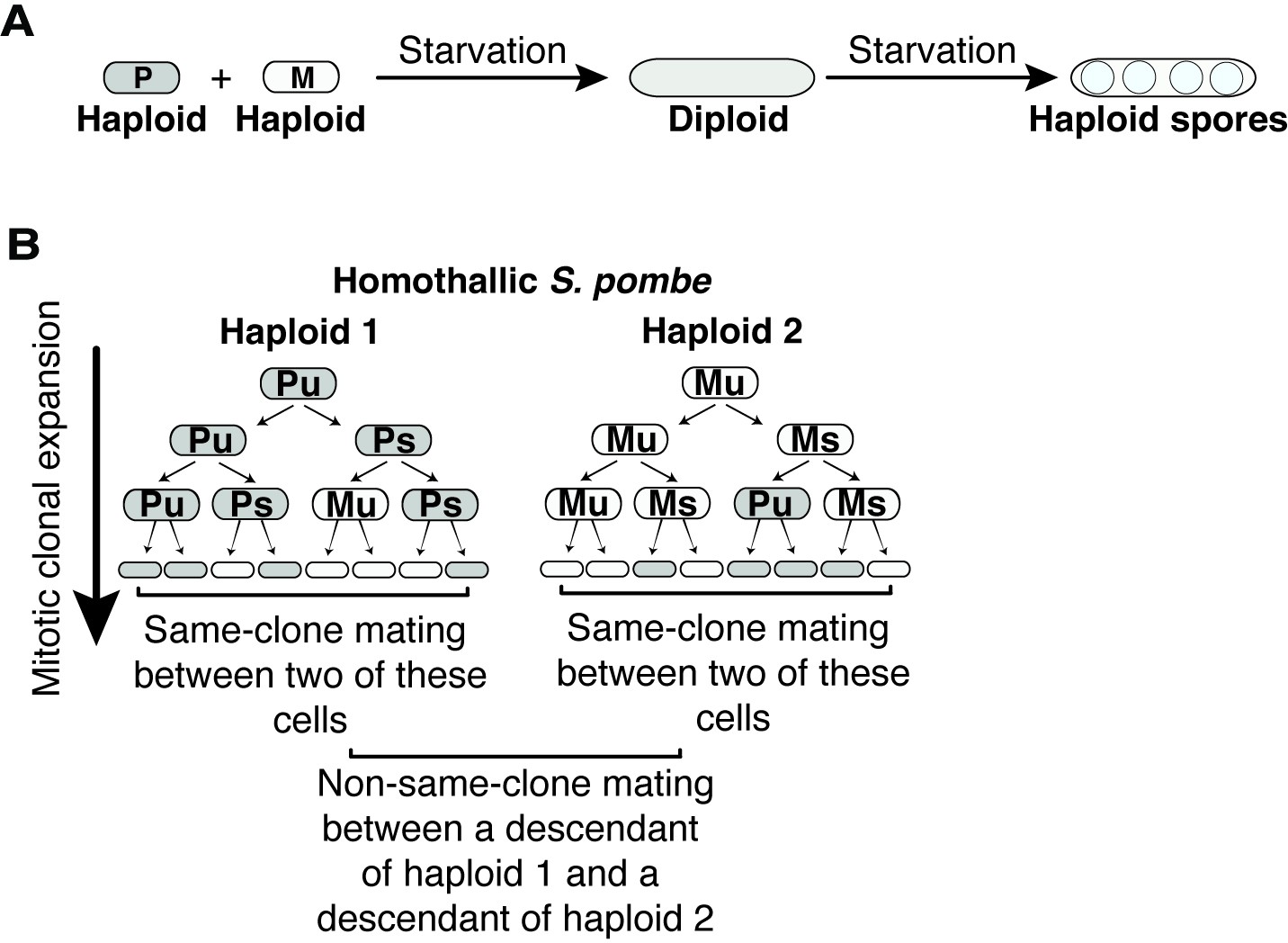
Sexual cycle of Schizosaccharomyces pombe.
(A) S. pombe haploid cells of compatible mating types h+ (P) and h- (M) can be induced to mate upon nitrogen starvation to form a diploid zygote. If starvation continues, the zygote undergoes meiosis to form haploid spores. (B) Patterns of mating-type switching in clonally expanding Sp cells. An unswitchable cell (u) divides to produce a switchable cell (s) and an unswitchable cell. Switchable cells divide to produce another switchable cell of the same mating type and an unswitchable cell of the opposite mating type. Cells that switch mating type (P to M or M to P) during mitotic growth are compatible within the clonal populations. Mating between cells derived from the same haploid progenitor are considered same-clone mating in this study. Mating events between descendants from different founder haploid cells are considered non-same-clone mating.
Figure 1—figure supplement 2
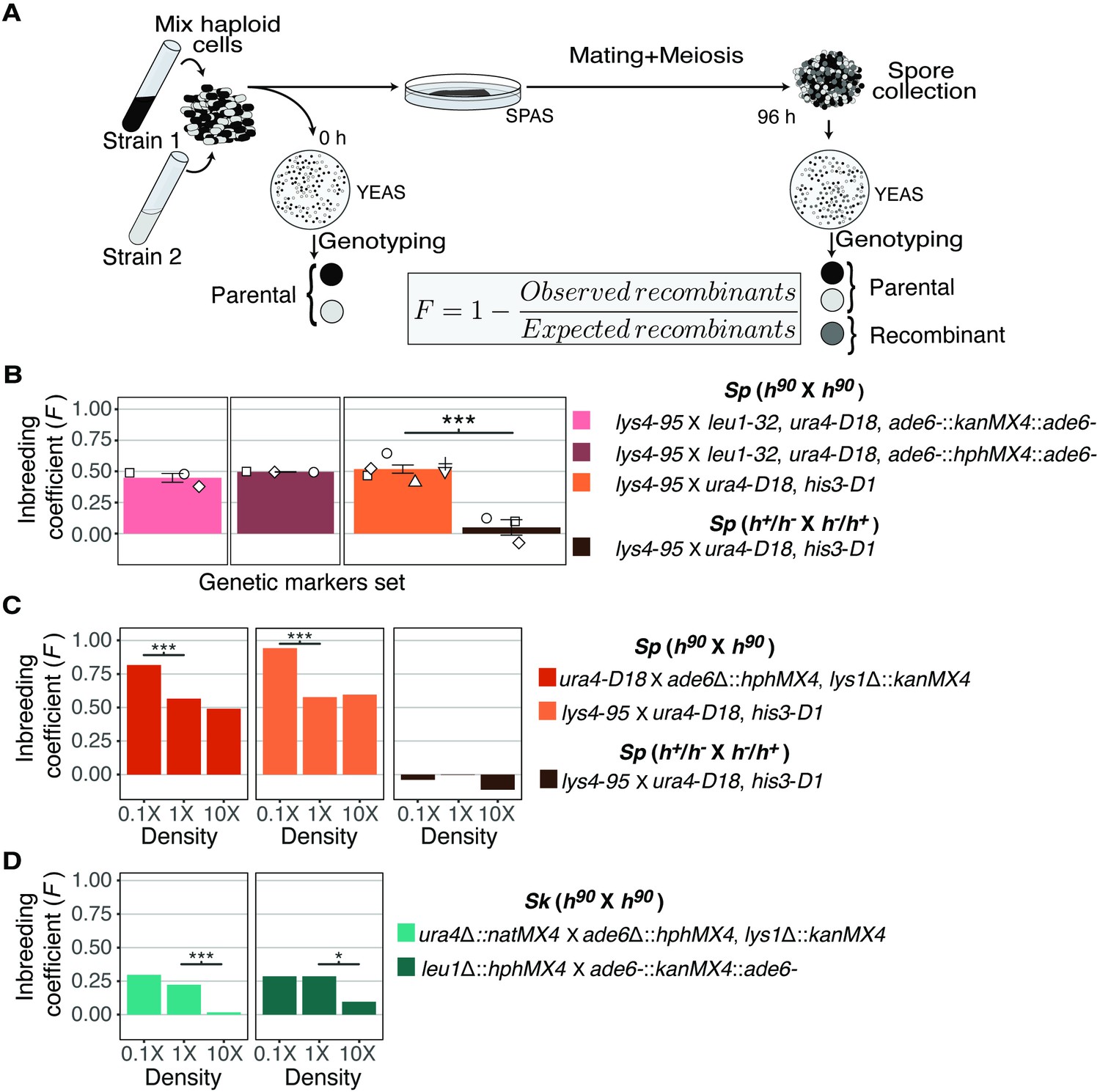
Inbreeding coefficients can be affected by cell density.
(A) Experimental strategy to infer inbreeding coefficient by genotyping the segregation of unlinked genetic markers. The composition of the starting population was measured by genotyping cells placed on rich medium (YEAS). Cells were also plated on SPAS, where they mate and undergo meiosis. After meiosis, spores were genotyped and we compared the expected number of recombinant progeny to the number observed to calculate the inbreeding coefficient (F). (B) Inbreeding coefficients calculated as described in (A) using the indicated genetic markers at standard 1× mating density. Each color indicates a different cross. *** indicates p-value < 0.005, One-tailed t-test on at least three biological replicates (open shapes). (C) Inbreeding coefficients calculated as described in (A) for Sp crosses plated at low (0.1×), standard (1×), and high (10×) density. *** indicates p-value < 0.005, G-test. Colonies were randomly sampled for each cross, 320 for left panel and 144 colonies for the second and third cross sets. (D) Inbreeding coefficients calculated as described in (A) for Sk crosses plated at low (0.1×), standard (1×), and high (10×) density. *** indicates p-value < 0.005, * indicates p-value < 0.05, G-test; 325 and 340 colonies were sampled from the crosses in the left and right panels, respectively.
-
Figure 1—figure supplement 2—source data 1
Raw data of allele transmission values reported in Figure 1—figure supplement 2.
Crosses shown in Figure 1—figure supplement 2 were genotyped before and after meiosis. The absolute and relative frequencies of each genotype were quantified. Segregation for each genetic marker is reported. From each cross, the list of recombinant genotypes are described. In Tables 1–3 on spreadsheet 1 (columns B–K) we show the genotypes, number of colonies counted, and initial frequencies of the two parents used in each cross represented in Figure 1—figure supplement 2B. In columns L, O, and R we show the expected frequency of Parent1, Parent2, and recombinants, respectively, predicted using Hardy-Weinberg. Columns M–Y show the results obtained after meiosis. In columns M–N, P–Q, and S–T we report the observed frequency and total number of colonies counted for Parent1, Parent2, and recombinants, respectively. In columns U–W (U–X for Table 3) we report the transmission frequency of each individual marker in the recombinants. The inbreeding coefficient for each cross is reported in column Y. In Tables 4–6 we show the numbers of each genotype obtained after meiosis for each replicate experiment. Parental genotypes are shown in white. Discordant genotypes are highlighted in blue at the bottom of each table. We also specify which experiments were performed manually and which were performed using robotics. Spreadsheet 2 shows similar data for the multiple density experiments shown in Figure 1—figure supplement 2C-D. Column Q also shows the G of fit G-test p-value.
- https://cdn.elifesciences.org/articles/70812/elife-70812-fig1-figsupp2-data1-v2.xlsx
Figure 1—figure supplement 3
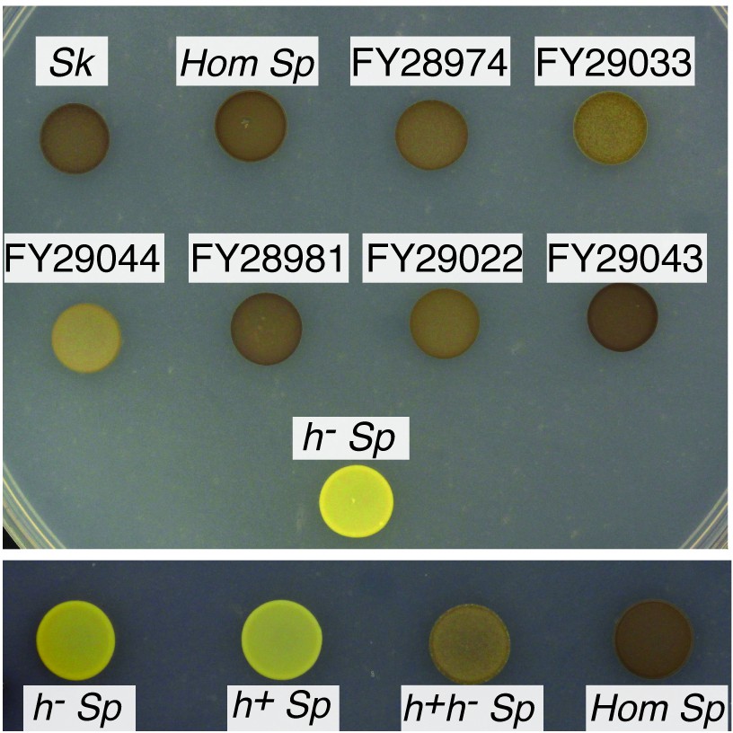
Homothallism of natural isolates.
Saturated cultures were spotted on SPAS to induce mating and meiosis. After 5 days at 25°C, cells were exposed to iodine vapor, which stains spores brown. The top panel shows natural isolates of homothallic (Hom) strains and h- Sp as a negative control. The bottom panel shows individual heterothallic strains, mixed complimentary heterothallic strains, and a homothallic isolate of Sp.
Figure 1—figure supplement 4
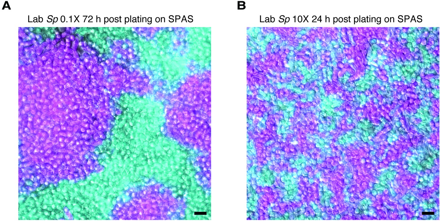
Density variation in plated cells.
Homothallic GFP (cyan)- and mCherry (magenta)-expressing cells were mixed, plated on SPAS, incubated at 25°C, and then imaged. On this medium, cells tend to divide until confluent prior to mating. When plated at low density (0.1×; A), cells form large clusters of clonal cells after ~72 hr. Cells mixed and plated at high density (10×; B) reach confluency after just 24 hr and form clusters with more contact zones between cells of different genotypes. Scale bars represent 10 µm.
Figure 2 with 7 supplements
Variation between mating behaviors in Sp and Sk cells.
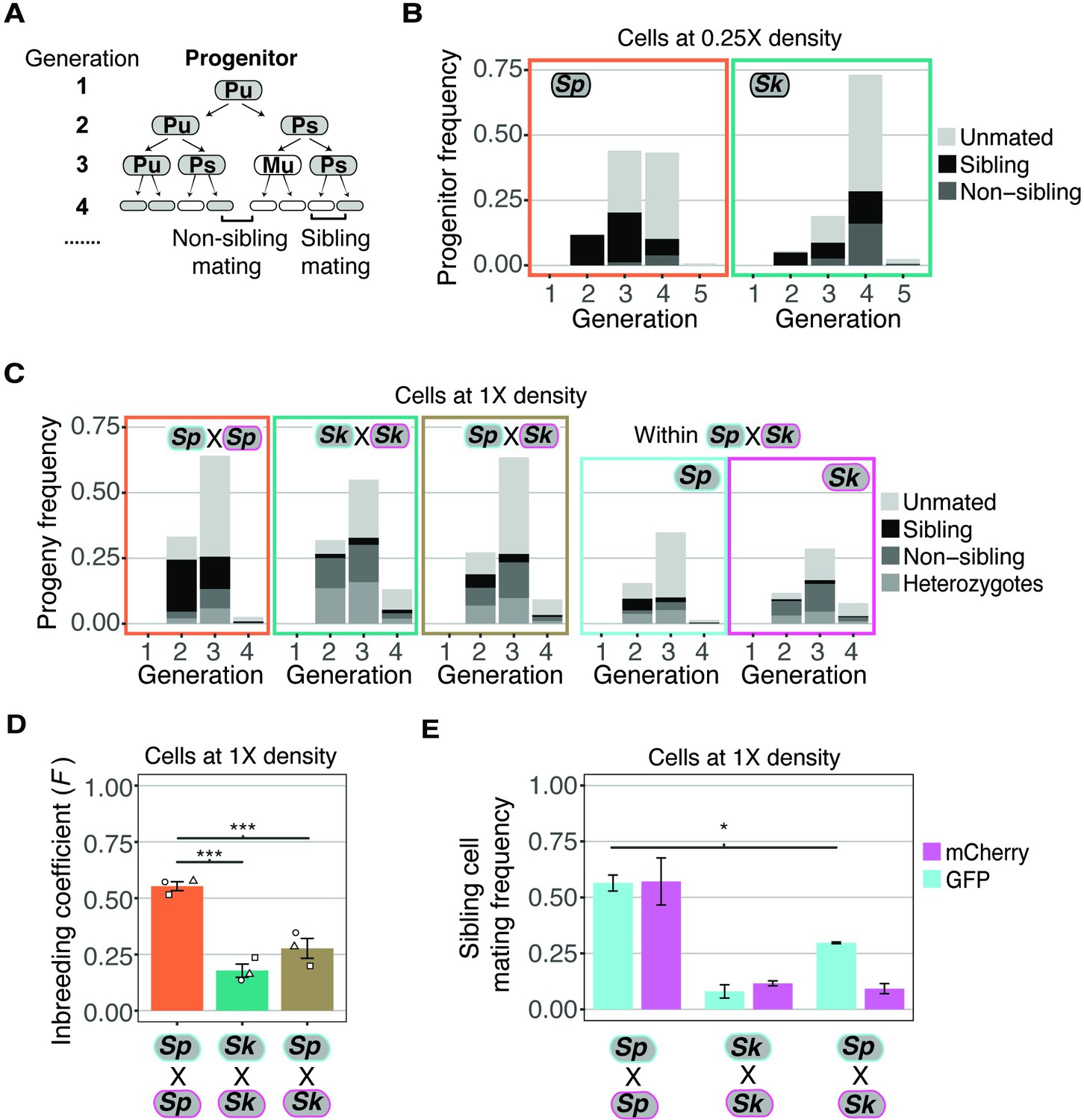
(A) Schematic showing cell divisions, switching, and mate choice in Sp. Mitotic generations are shown on the left. Cells are either h+ (P) or h- (M) and their status is switchable (s) or unswitchable (u). (B) Division and mating phenotypes of wildtype Sp and Sk cells plated at low cell density (0.25×) on SPA plates. Single founder cells and their descendants were monitored through time-lapse imaging. Mating patterns were categorized until the end of the generation in which the first mating event occurred. The data presented were pooled from two independent time-lapses in which over 400 founder cells were tracked. (C) Division and mating phenotypes of fluorescently labeled Sp and Sk cells plated at standard (1×) density on SPA plates. Individual cells were monitored until the population reached a typical mating efficiency for the specific cross and the mate choice of their progeny and the mitotic generation of those events was classified. The cells labeled with GFP are indicated with a cyan line around the cell whereas the mCherry-labeled cells are outlined in magenta. Pooled data from two independent experiments are presented, with 286 cells scored from each experiment. In the cross of Sp (GFP) and Sk (mCherry), we present an additional plot (far right) in which the fate of each founder is separated by isolate. (D) Inbreeding coefficient calculated from still images of cells plated at 1× density on SPA. *** indicates p-value < 0.005, multiple t-test, Bonferroni corrected. At least three biological replicates per isolate are shown (open shapes). (E) Breakdown of sibling cell mating by fluorophore in the indicated crosses from C. * indicates p-value = 0.04, one-tailed t-test comparing isogenic and mixed Sp cells from two videos.
Figure 2—figure supplement 1

Mating-type switching dual reporter assay using mating-type-specific promoters in Sp.
(A–C) Cells expressing both YFP under control of the h- cell-specific mfm3 promoter and CFP under control of the h+ cell-specific map2 promoter (from Jakočiūnas et al., 2013) were visualized using time-lapse microscopy. Image contrast was enhanced due to signal bleaching at later timepoints and to better distinguish switching events from background. (A–B) Switching events (CFP to YFP and YFP to CFP) were generally only visible after progenitor cells produced eight clonal descendants. Progenitors and clonal descendants are highlighted with dotted lines. The observed pattern of fluorophore switching is different than the expected mating-type switching pattern where one out of four cells derived from the same progenitor is expected to have the opposite mating type as the other three cells (Figure 1—figure supplement 1B). (A) Cells were grown for 24 hr in PM-N+ ade + leu, washed 3× in PM-N, then plated at 0.5× to SPA+ ade + leu. One-hour post-plating a time-lapse was recorded using a Nikon Ti spinning disc microscope at 25°C. Arrows indicate cells that switched fluorescent protein expression. (B) Cells were grown for 24 hr in PM-N+ ade + leu, washed 3× in ddH2O, then plated at 1× to SPAS; 12 hr post-plating a time-lapse was recorded using a Nikon Ti2-E widefield microscope at 25°C. In three of the four cell divisions that led to the eight-cell stage, a fluorophore switching event occurred. The fourth cell may have switched prior to the division as both sister cells appear to have switched. These observations also violate the current model of mating-type switching (Figure 1—figure supplement 1B). Arrows indicate cells involved in mating after switching fluorescent protein expression. (C) Sibling cells expressing CFP mated (dashed line) without an accompanying fluorophore shift. Cells were treated and time-lapses recorded as in (B). The two mating partners are highlighted with dotted lines. Scale bars represent 10 μm.
-
Figure 2—figure supplement 1—source data 1
Original file of the full raw unedited gel shown in Figure 2—figure supplement 1B.
- https://cdn.elifesciences.org/articles/70812/elife-70812-fig2-figsupp1-data1-v2.pdf
-
Figure 2—figure supplement 1—source data 2
Original file of the full raw unedited gel shown in in Figure 2—figure supplement 1B with relevant band labeled.
- https://cdn.elifesciences.org/articles/70812/elife-70812-fig2-figsupp1-data2-v2.tiff
Figure 2—figure supplement 2
Mating-type locus variation in Schizosaccharomyces pombe isolates.
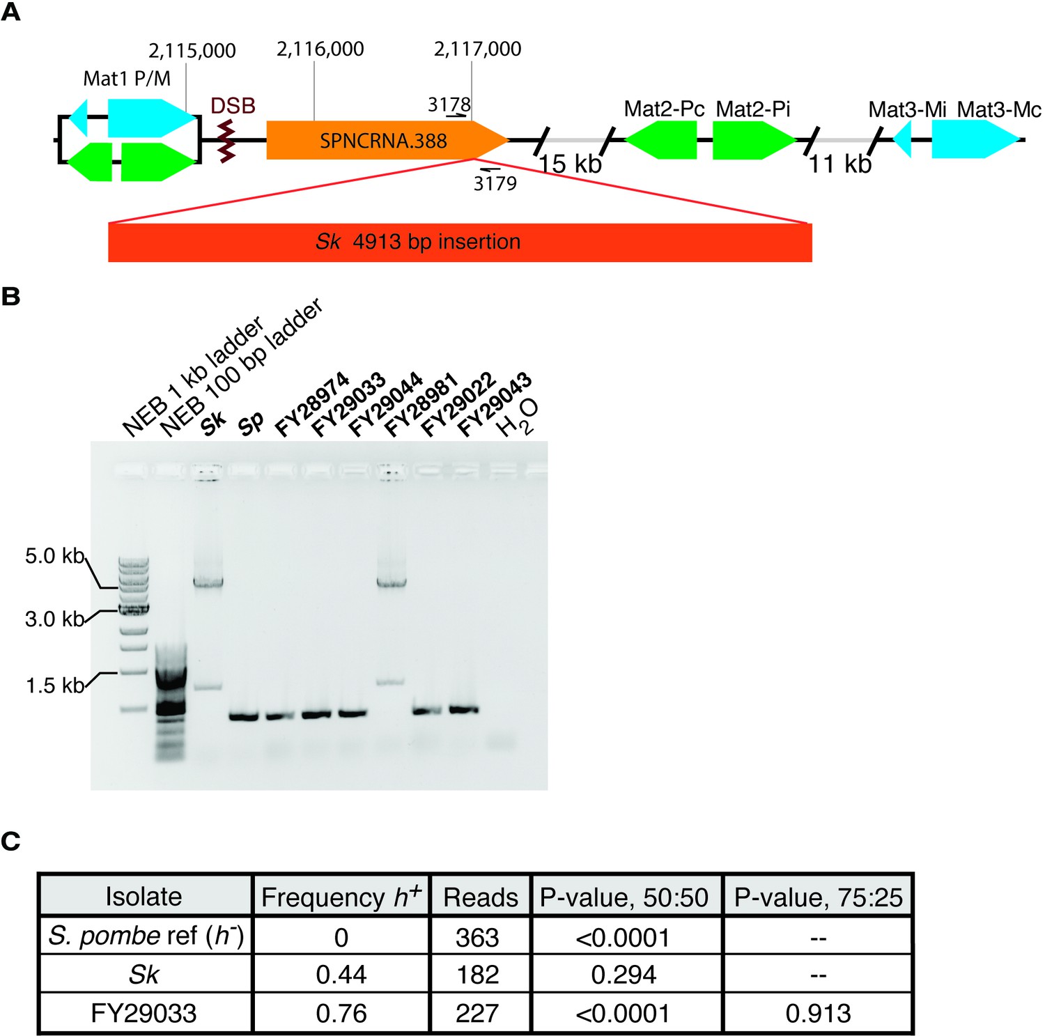
(A) Schematic representation of the mating-type locus. We found a 5 kb insertion of transposon sequences in the Sk isolate using published Illumina mate-pair sequencing data (Eickbush et al., 2019). The insert is within SPNCRNA.388, near the double-strand break site (DSB) where switching initiates. (B) PCR amplification of the 5 kb insertion using the oligos 3178 and 3179 shown in (A) suggests the insertion is also in the FY28981 isolate. (C) We aligned long nanopore sequencing from the indicated strains to the Sp reference genome mat locus, which is h-. We then quantified the frequency of h+ alleles from the aligned reads. We used Fisher’s exact tests to compare our observations to the indicated ratios.
Figure 2—figure supplement 3
Variation in cell division and asci phenotypes in natural isolates.
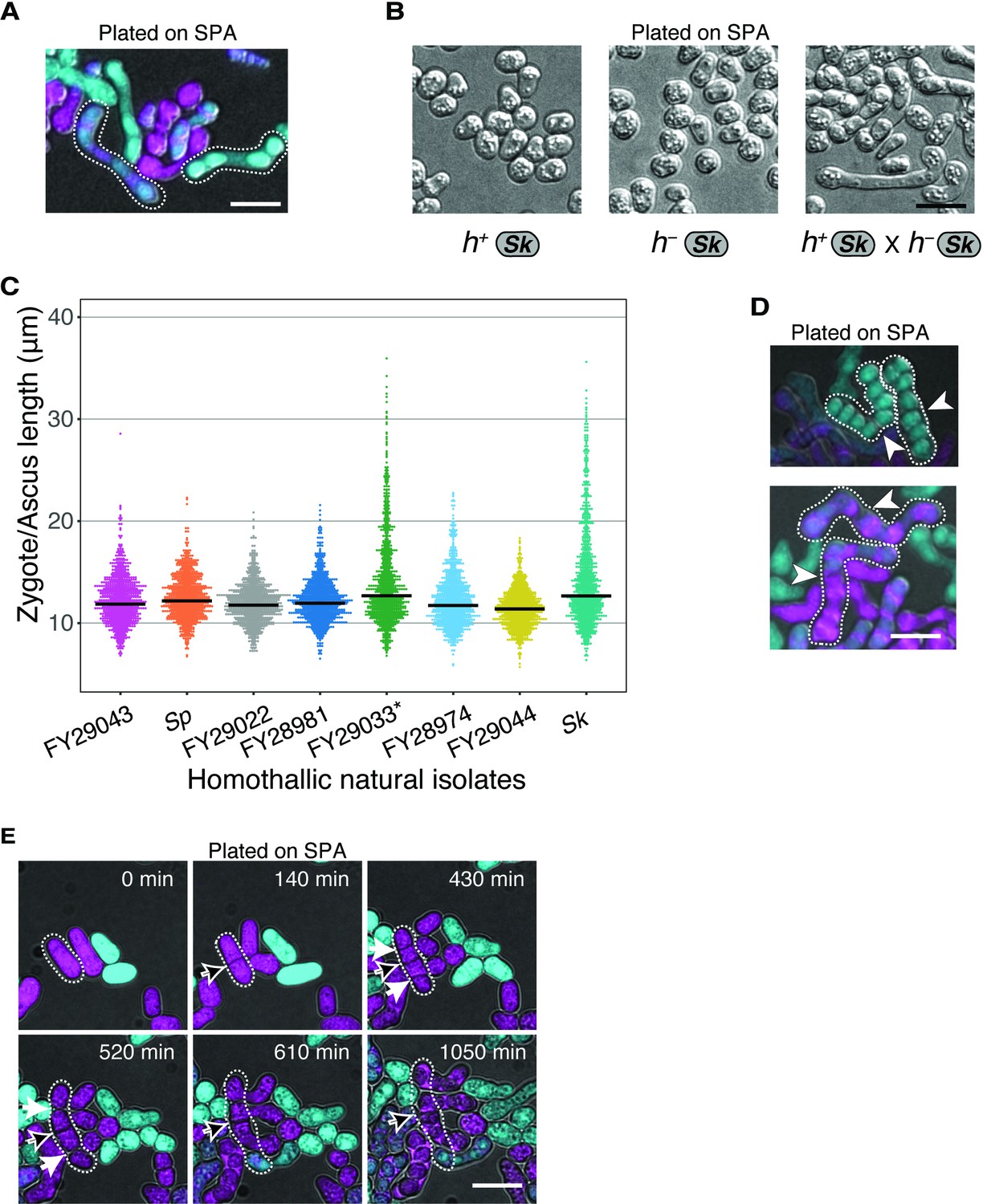
(A) Examples of Sk-long asci formed by GFP- and mCherry-expressing cells mated on SPA. (B) Sk cells of each mating type were plated to SPA plates individually or in combination and imaged after 48 hr at 25°C. Cells only form long projections (shmoos) in response to cells of the opposite mating type. (C) Tip-to-tip length (tracing through the center of the cells) of zygotes and asci of distinct natural isolates. Cells were plated on SPA and incubated for 24 hr at 25°C. *FY29033 cells showed a clumpy phenotype upon nitrogen starvation; 336 sampled cells from three independent biological replicates. (D) Examples of Sk asci fused at uncleaved septa. White arrows indicate uncleaved septa. (E) Time-lapse showing Sk cells with a septum (black arrow) that remained uncleaved after two rounds of fission. Additional septa (white arrows) are also shown that cleaved prior to mating. Scale bar represents 10 µm.
Figure 2—figure supplement 4
Mating efficiency and asci length of Sp/Sk heterozygotes.
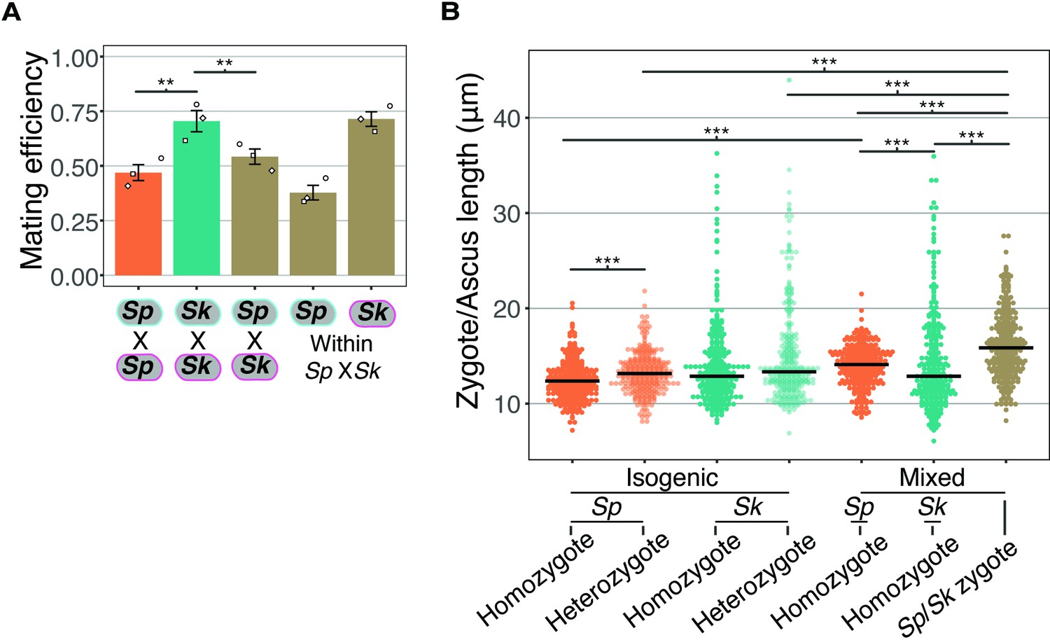
(A) Mating efficiency calculated from still images taken after 24 hr on SPA at 25°C from isogenic and mixed isolate crosses. The open shapes represent values from three biological replicates per cross. ** indicates p-value < 0.01, t-test. (B) Length of zygotes/asci from isogenic and mixed isolate crosses of Sp and Sk. Cells were plated on SPA at 1× density and incubated for 24 hr at 25°C before being imaged. For each category (e.g., homozygote) of zygote, 100 cells were sampled from three independent biological replicates. Multiple Wilcoxon rank sum tests, Bonferroni corrected; ***, p-value < 0.005.
Figure 2—figure supplement 5
Mostly additive phenotypes in crosses between natural isolates.
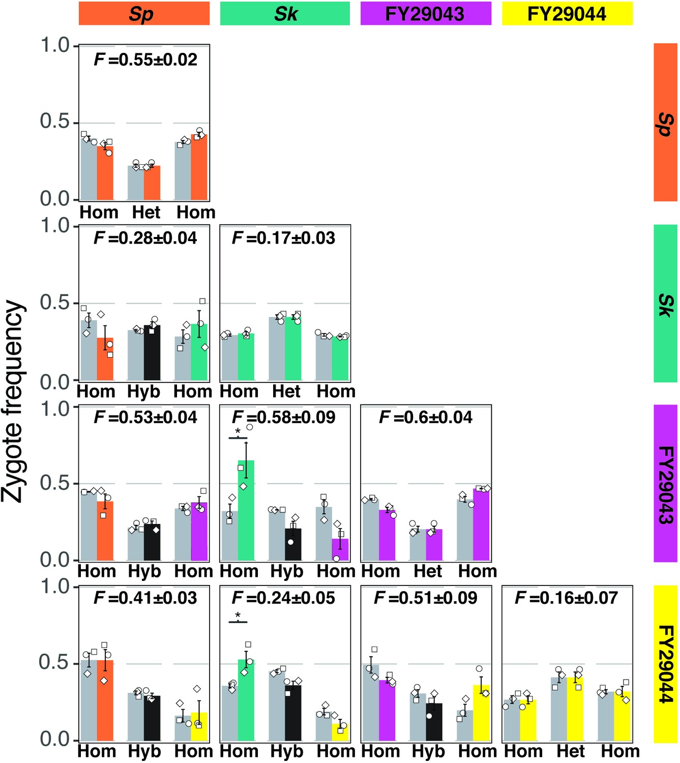
Four natural isolates with distinct mating efficiencies and inbreeding coefficients were mixed and mated in all pair-wise combinations. After 24 hr on SPA at 25°C, cells were imaged and the mating efficiencies and inbreeding coefficients were calculated using fluorescent markers scored from still images, obtained as in Figure 1A. On the outer diagonal are isogenic crosses color-coded with the respective natural isolate. For the non-isogenic crosses, the observed homozygotes (hom) are color-coded by the respective parent isolate. The observed frequencies of hybrid (hyb) zygotes and asci are plotted in black. The expected values (gray bars) account for the inbreeding coefficient and mating efficiency from each isolate assuming the parental phenotypes are additive. Inbreeding coefficients (F values) and standard error (±) for each cross are indicated above each plot. The open shapes represent experimental replicates. * indicates p-value < 0.05, one-tailed t-test.
Figure 2—video 1
Homothallic Sp mating video.
Homothallic Sp cells plated on mating inducing media (SPA) were recorded for 24 hr. Cells labeled with constitutively expressing fluorophores mCherry (magenta) or (GFP) were mixed in equal proportion 1× standard cell density.
Figure 2—video 2
Homothallic Sk mating video.
Homothallic Sk cells plated on mating inducing media (SPA) were recorded for 24 hr. Cells labeled with constitutively expressing fluorophores mCherry (magenta) or (GFP) were mixed in equal proportion at 1× standard cell density.
Figure 3 with 1 supplement
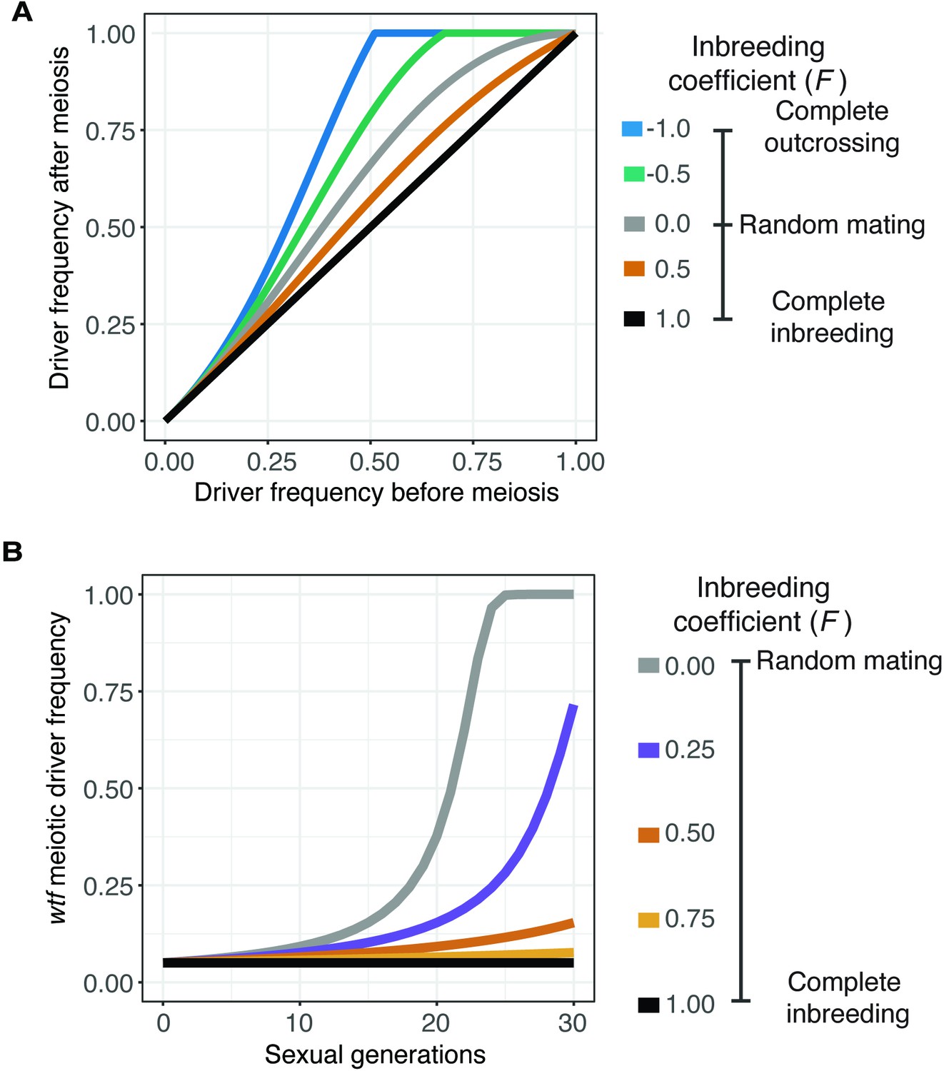
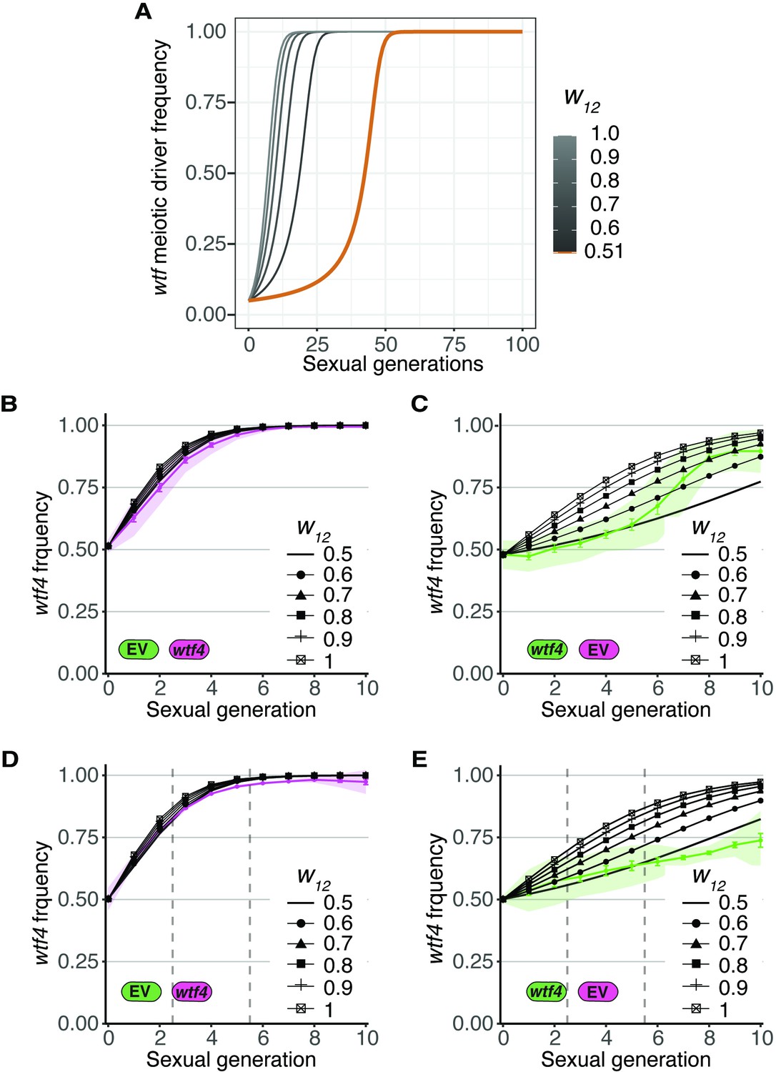
Inbreeding is predicted to slow the spread of a wtf driver.
We assumed a 0.98 transmission bias favoring the wtf driver and a fitness of 0.51 in wtf+/wtf- heterozygotes. We assumed that homozygote fitness is 1. We simulated the spread of a wtf driver for 30 generations. (A) Change of wtf meiotic driver frequency after a single meiosis assuming varying levels of inbreeding. (B) The spread of a wtf driver in a population over time assuming varying levels of inbreeding.
Figure 3—figure supplement 1
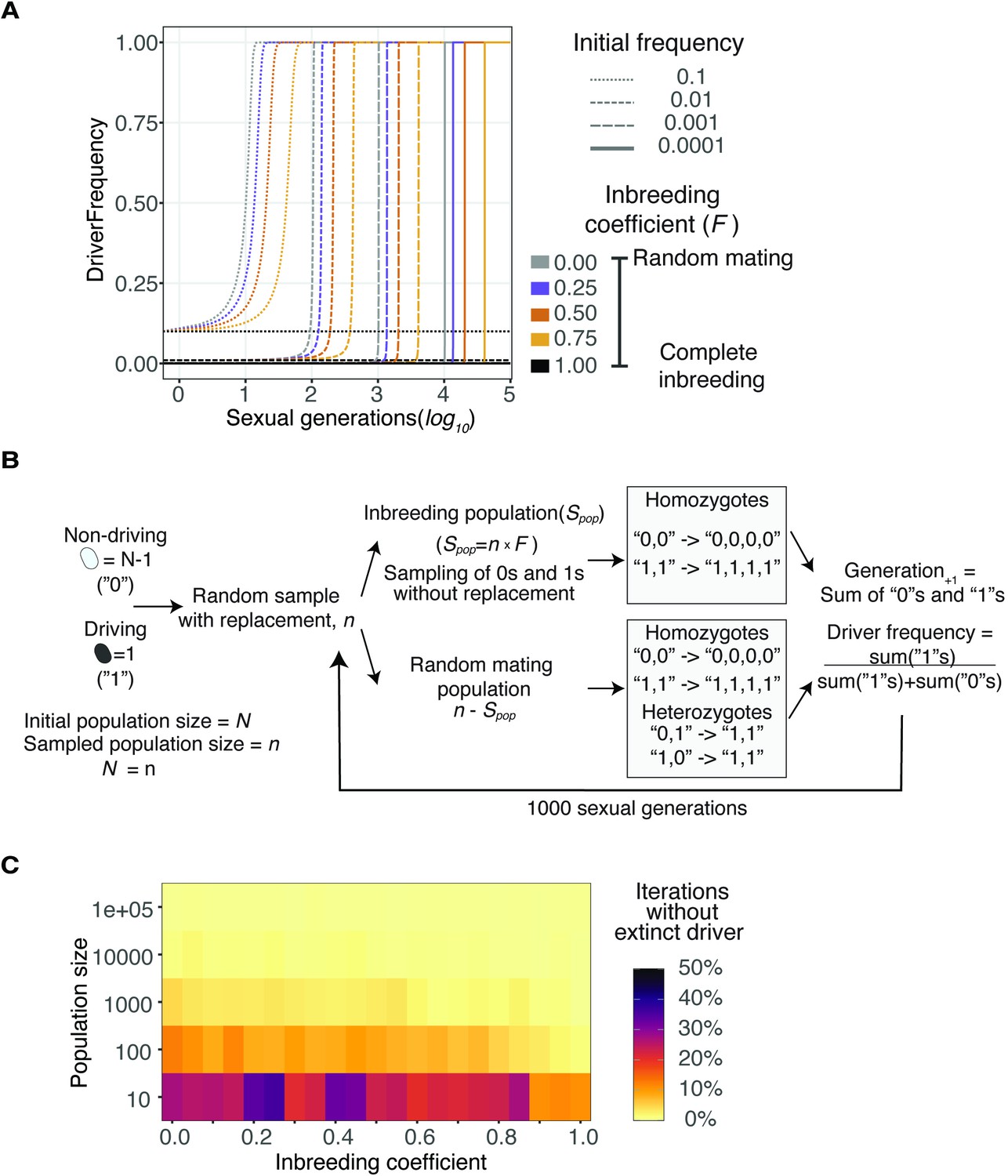
Spread of a wtf driver under varying initial frequencies and population sizes.
(A) Distinct initial frequencies (line type) were simulated under varying inbreeding coefficients (colors) to evolve throughout multiple sexual generations. Populations with complete inbreeding remained constant, while all populations with an initial driver frequency greater than 0 reached fixation. (B) Evolution of a single cell carrying a wtf meiotic driver in different population sizes under a Wright-Fisher model (see Materials and methods). Driving cells are represented as ‘1’s and non-driving as ‘0’s. We introduced only one driver cell among the distinct population sizes. We repeated the process over 1000 sexual generations by 1000 iterations. (C) Proportion of iterations that did not show extinction of the driver (i.e., either fixed or still evolving).
Figure 4 with 2 supplements
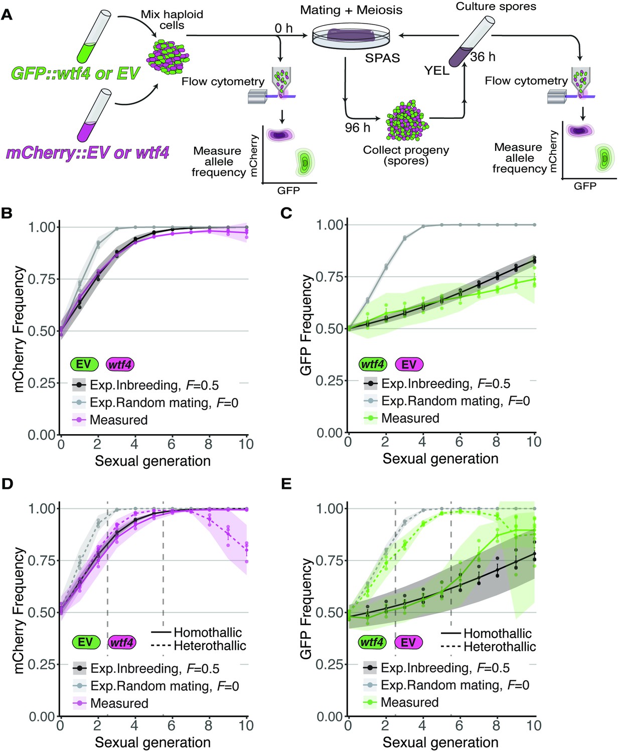
Inbreeding slows the spread of the wtf4 meiotic driver in homothallic strains.
(A) Experimental strategy to monitor allele frequency through multiple generations of sexual reproduction. GFP (green) and mCherry (magenta) markers are used to follow empty vector (EV) alleles or the wtf4 meiotic driver. Starting allele frequencies and allele frequencies after each round of sexual reproduction were monitored using cytometry. (B) Homothallic population with mCherry marking wtf4 and GFP marking an EV allele. Allele dynamics were predicted using drive and fitness parameters described in the text assuming an inbreeding coefficient of 0.5 (black lines) and random mating (inbreeding coefficient of 0; gray lines). The individual spots represent biological replicates and the shaded areas around the lines represent 95% confidence intervals. (C) Same experimental setup as in (B), but with mCherry marking the EV allele and GFP marking wtf4. (D–E) Repeats of the experiments shown in (B) and (C) with two alterations. First, these experiments tracked heterothallic populations (dotted lines) in addition to homothallic cells (solid lines). Second, the populations were sorted by cytometry at generations 3 and 5 (vertical long-dashed lines) to remove non-fluorescent cells.
Figure 4—figure supplement 1
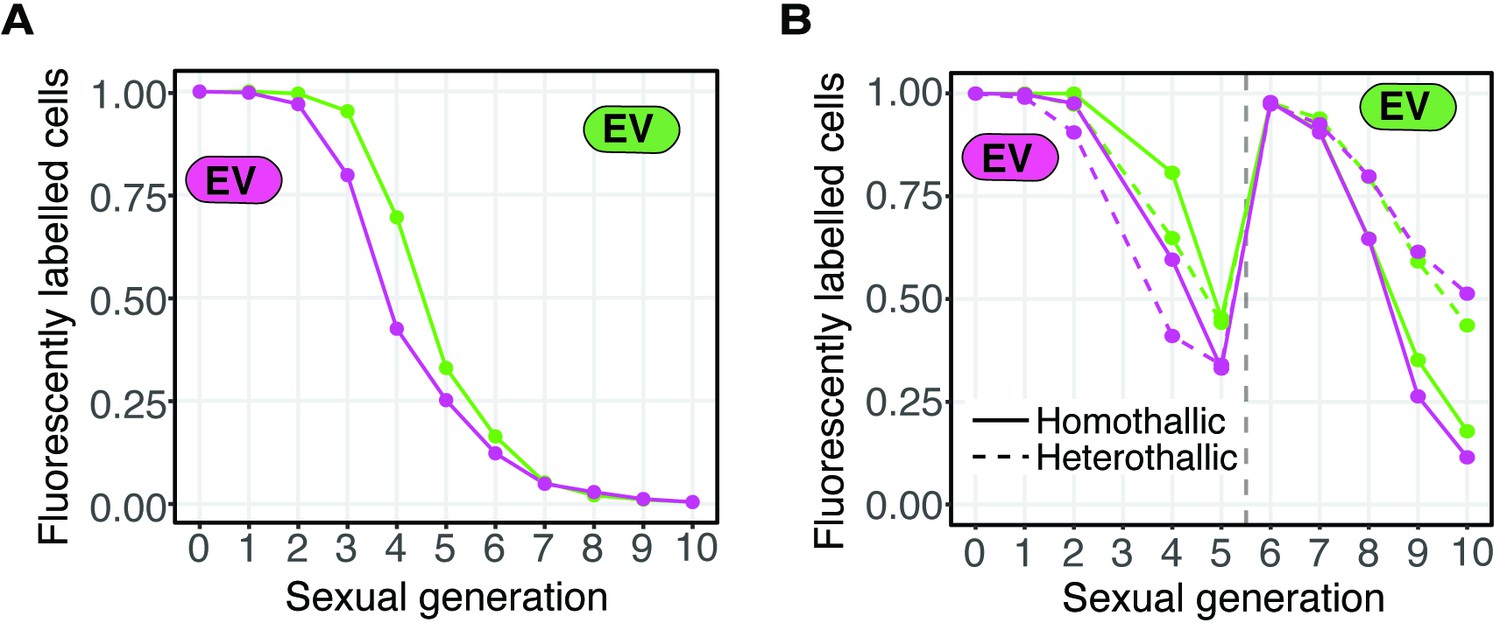
Loss of fluorescent markers in experimental evolution analyses.
(A) Fluorescent marker loss from cell populations carrying only one type of fluorescent marker (GFP or mCherry) linked to an empty vector (EV). Cells were grown as in Figure 4A in parallel to the cell populations depicted in Figure 4B–C. (B) Similar to A, but both heterothallic and homothallic cells were analyzed in parallel to the cell populations depicted in Figure 4D–E. The cells were sorted after generation five to remove non-fluorescent cells (vertical gray dotted line).
Figure 4—figure supplement 2
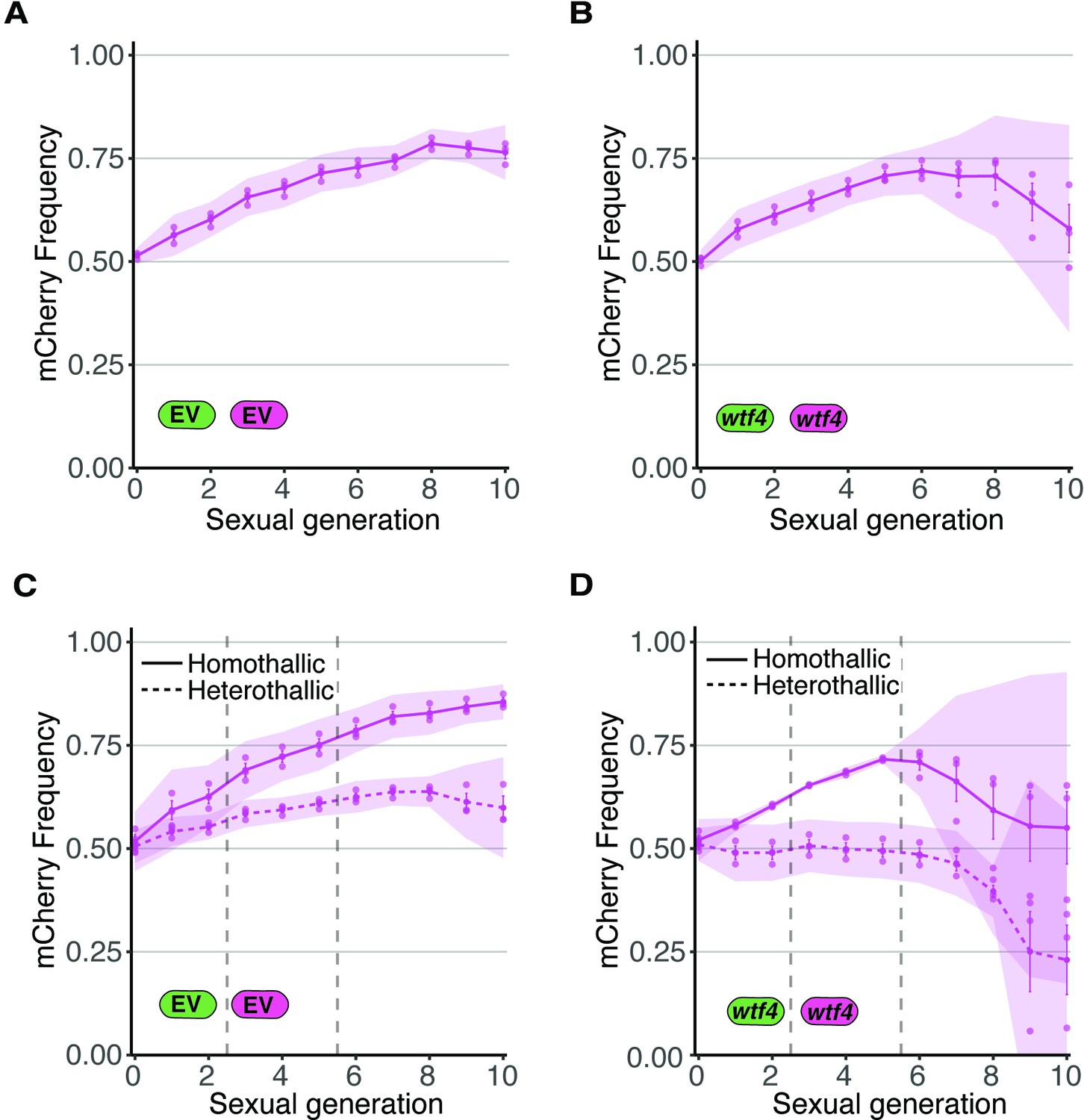
Allele transmission in homozygous control homothallic and heterothallic populations.
(A) Homothallic population with both mCherry and GFP marking empty vector (EV) alleles. The individual spots represent biological replicates and the shaded areas around the lines represent 95% confidence intervals. (B) Same experimental setup as in (A), but with both markers linked to a wtf4 allele. (C–D) Repeats of the experiments shown in (A) and (B) with two alterations. First, these experiments tracked heterothallic populations (dotted lines) in addition to homothallic cells (solid lines). Second, the populations were sorted by cytometry at generations 3 and 5 (vertical long-dashed lines) to remove non-fluorescent cells.
Figure 5 with 2 supplements

Inbreeding purges wtf drivers with linked deleterious alleles.
(A) Modeling the predicted impacts of inbreeding, the fitness of the driving haplotype, and the initial frequency of the driver on the spread of a wtf driver linked to a deleterious allele with low dominance (h = 0.083) in a population. The circle indicates the predicted initial frequency necessary for the GFP:wtf4+ allele to spread in a population when mated at standard (1×) density where F = 0.5. The diamond indicates the predicted initial frequency necessary for the GFP:wtf4+ allele to spread in a population when mated at low (0.1×) density where F = 0.8–0.95 measured in Figure 1—figure supplement 2C. (B) Experimental analyses of the impacts of inbreeding and the initial driver frequency on the spread of the GFP:wtf4+ allele in a population. A single biological replicate was used for each initial frequency and inbreeding condition.
Figure 5—figure supplement 1
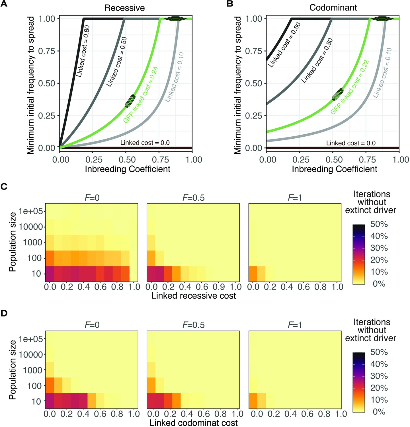
Evolution of wtf meiotic drivers in populations for recessive and codominant costs.
(A–B) Modeling the predicted impacts of inbreeding, the fitness of the driving haplotype, and the initial frequency of the driver on the spread of a wtf driver linked to a completely recessive (A); h = 0 or codominant (B); h = 0.5 deleterious allele. The oval indicates the predicted initial frequency necessary for the GFP::wtf4+ allele to spread in a population when mated at standard (1×) density where F = 0.5. The diamond indicates the predicted initial frequency necessary for the GFP::wtf4+ allele to spread in a population when mated at low (0.1×) density where F = 0.8–0.95 measured in Figure 1—figure supplement 2C. (C–D) Evolution of a population in which a single cell carrying a wtf driver is introduced under a Wright-Fisher model with different fixed population sizes. Simulations were performed under three inbreeding coefficients (F). We simulated for 1000 generations and 1000 iterations for each condition. The proportion of iterations that maintained the meiotic driver are shown for simulations in which the linked costs were recessive (h = 0) in (B) or codominant (h = 0.5) in (D).
Figure 5—figure supplement 2
Assessing if wtf+ spores gain fitness as a result of spore killing.
(A) Simulation of the evolution of a wtf meiotic driver starting at a frequency of 0.05 in the population. This analysis is similar to that presented in Figure 3B, except the inbreeding coefficient (F) was held constant at 0.5 and fitness values of wtf driver heterozygotes greater than 1 were considered. A driver heterozygote with fitness of 0.51 (as in Figures 3—5, and Figure 5—figure supplement 1A-B) is shown with an orange line. Increasing the fitness of the driver heterozygote w12 >0.51 (gray lines) results in a faster spread of the meiotic driver. (B–E) Comparison of the wtf4 predicted meiotic driver spread assuming different driver heterozygote fitness values (black lines) to the experimentally observed values (colored lines). (B) Observed values form Figure 4B compared to multiple relative heterozygote fitness. (C) Observed values form Figure 4C compared to multiple relative heterozygote fitness. (D) Observed values form Figure 4D compared to multiple relative heterozygote fitness. Cell-sorting events are indicated with vertical gray lines. (E) Observed values form Figure 4E compared to multiple relative heterozygote fitness. Cell-sorting events are indicated with vertical gray lines.
Additional files
-
Supplementary file 1
Yeast strains used in this study.
Strains used and created in this study are listed.
- https://cdn.elifesciences.org/articles/70812/elife-70812-supp1-v2.xlsx
-
Supplementary file 2
Plasmids used in this study.
- https://cdn.elifesciences.org/articles/70812/elife-70812-supp2-v2.xlsx
-
Supplementary file 3
Oligo table.
Oligos used in this study.
- https://cdn.elifesciences.org/articles/70812/elife-70812-supp3-v2.xlsx
-
Transparent reporting form
- https://cdn.elifesciences.org/articles/70812/elife-70812-transrepform1-v2.docx
Download links
A two-part list of links to download the article, or parts of the article, in various formats.
Downloads (link to download the article as PDF)
Open citations (links to open the citations from this article in various online reference manager services)
Cite this article (links to download the citations from this article in formats compatible with various reference manager tools)
Diverse mating phenotypes impact the spread of wtf meiotic drivers in Schizosaccharomyces pombe
eLife 10:e70812.
https://doi.org/10.7554/eLife.70812


