Emerging dynamics from high-resolution spatial numerical epidemics
Abstract
Simulating nationwide realistic individual movements with a detailed geographical structure can help optimise public health policies. However, existing tools have limited resolution or can only account for a limited number of agents. We introduce Epidemap, a new framework that can capture the daily movement of more than 60 million people in a country at a building-level resolution in a realistic and computationally efficient way. By applying it to the case of an infectious disease spreading in France, we uncover hitherto neglected effects, such as the emergence of two distinct peaks in the daily number of cases or the importance of local density in the timing of arrival of the epidemic. Finally, we show that the importance of super-spreading events strongly varies over time.
Introduction
Mathematical modelling is a powerful tool to describe infectious disease epidemics, for example when combined to statistical modelling, and also to understand ongoing processes (Kermack and McKendrick, 1927; Keeling and Rohani, 2008). The recent COVID-19 pandemic has put in the spotlights the importance of mathematical epidemiology models to elaborate intervention strategies (Adam, 2020). These models face important challenges such as stochasticity, spatial structure, or individual heterogeneity. In the initial stages of an outbreak, the effect of spatial structure is minimal because transmission chains are largely independent, but individual heterogeneity and stochasticity have major effects (Trapman et al., 2016; Britton and Scalia Tomba, 2019). As the epidemic unfolds and host become immune, accounting for the exact shape of local contact networks matters increasingly (Keeling and Rohani, 2008). Several approaches have been developed in epidemiological models to capture spatial structures, for example meta-populations (Grenfell and Harwood, 1997), moment equations (Lion, 2016), or contact networks (Pellis et al., 2015). However, one of their limitation is that they simplify the geographical structure (sometimes ignoring it completely), which can lead to overlooking emerging patterns and complicate the practical implementation of local policies.
Agent-based simulation (ABS), where individuals are modelled explicitly, represent a seducing option to achieve a high degree of realism, from a biological and environmental point of view (Abar et al., 2017), but their routine use in public health faces three major limitations. First, ABS are very computationally demanding (Eubank et al., 2004), which restrains the total number of agents that can be simulated. The second limitation comes from the model dimensionality and the introduction of numerous parameters, many of which are poorly informed and set in an ad hoc manner, to capture individual heterogeneity. A third limit resides in the way the geographic structure is implemented into the simulation.
The recent SARS-CoV-2 pandemic has led to the creation or the re-implementation of ABS that alleviate some of the limitations. For instance, some of these simulations were used to introduce biological details into the model that would require numerous equations in an analytical approach (see e.g. Kerr et al., 2021). Other ABS introduced some spatial structure to tackle generic questions, such as the impact of individual movement on epidemic spread. Given the nature of the questions asked and also given the additional types of structures in the model, for instance in terms of individual ages of households, these simulations typically simplified the spatial structure using contact networks (see e.g. Hinch et al., 2021, Kerr et al., 2021 at a city level, or Aleta et al., 2020 for unstructured network regenerated by contact tracing). To our knowledge, few ABS feature high-resolution geographical scale. There are exceptions and, for instance, Smieszek et al., 2011 analyse the spread of influenza virus in Switzerland using an ABS using a grid with 500x500m resolution. Rockett et al., 2020 perform a similar analysis in Australia using the 2310 level 2 statistical areas Also, the recent work by The GAMA platform allows one to combine a detailed epidemiological model with a high geographical resolution (Taillandier et al., 2019). In general, achieving a high degree of geographical realism for a large number of agents is an open challenge in epidemiology.
Here, we introduce Epidemap, a novel numerically efficient agent-based method that addresses many limitations of current ABS platforms. In particular, it can simulate infectious diseases epidemic scenarios at the scale of a whole country by combining high-resolution geographical structure, demographic information, and mobility statistics. Practically, this is achieved by using high-performance computing (HPC) techniques, building-level spatial data from the OpenStreetMap (OSM) project (Haklay and Weber, 2008), and sophisticated mobility models (Barbosa et al., 2018). Overall, in addition to the number and age of the hosts (which is informed by the demography) and the initial conditions (number of infected hosts at ), these simulations only require seven parameters (see Table 2).
To illustrate the power and flexibility of the platform, we study the transmission dynamics of an (uncontrolled) epidemic of respiratory infections in France. The biological features of the epidemiological model originate from a discrete-time SARS-CoV-2 transmission model parameterised with national hospital data (Sofonea et al., 2021). Given the general focus of the study, we voluntarily focus more on the transmission dynamics than on the clinical dynamics but both are implemented. We analyse the output of 100 stochastic simulations from epidemic emergence to extinction, that is, approximately 1 year. A typical simulation generates daily mobility patterns for 66 million individuals at the scale of buildings and lasts less than 2 hr. Further details about the simulation specifications and comparisons with existing platforms can be found in the Materials and methods.
In the simulations, which are summarised in Figure 1 and detailed in the Materials and methods, each individual is assigned to a residency building and can visit two other buildings every day. These buildings are chosen at random based on a distance kernel (see the Materials and methods). If more than one individual visits the building the same day, transmission can occur. The life-history of the infection is parameterised using data from the COVID-19 epidemic in France (Sofonea et al., 2021). Note that most of the parameters are required to simulate Intensive Care Unit (ICU) bed occupancy dynamics, which do not affect the transmission dynamics. Given the general scope of this study, we assume that recovered individuals have perfect immunity for the duration of the simulation (i.e. a classical Susceptible Infected Recovered (SIR) epidemiological formalism) and that all simulations are initialised with 15 infected individuals in Paris to avoid premature random epidemic extinction. Similarly, although the simulation tracks the age of the individuals, which is distributed geographically according to national demographics data (INSEE, 2020), following a parsimony principle, we assume that it does not affect the mobility or the transmission model (but age does affect the clinical model).

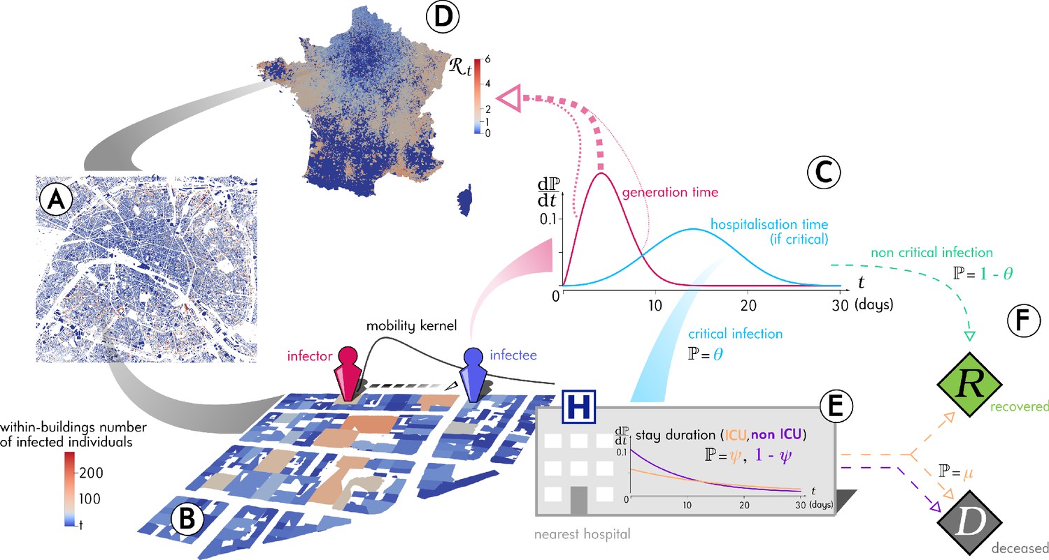
Outline of the Epidemap simulation framework.
(A) The 66 millions inhabitants of metropolitan France are explicitly mapped to housing buildings following cartographic and demographic data. (B) At each time point of the simulation, the number of infected individuals in each building of the country is recorded, as well as the time past since each got infected (the panel shows the Paris area). (C) Every day, individuals can randomly move from their home to other buildings according to a mobility kernel and meet other people. If an infected individual encounters a susceptible host, a transmission event can occur. (D) The contagiousness of a infected individual varies depending on the time since infection. (E) A small fraction of infected individuals develop a critical form of the disease that requires their hospitalisation to the nearest facility. Clinical dynamics can be assumed not to affect transmission dynamics because more than 95% of the secondary transmission events occur before hospital admission.
Epidemap simulations do not attempt to reconstruct a past epidemic. They are not conceived either to perform statistical parameter inference. Their main goal is to simulate realistic scenarios to better understand how mobility patterns, geographical structure, and infectious disease biology interact to shape epidemic spread and to optimise public health responses.
Results
Figure 2 shows the output of the dynamics at the national level for 100 stochastic simulations. For optimal readability, the dates are aligned based on the day where ICU-occupancy reaches a value of 700. With our minimal parameterisation, we see that the basic reproduction number, which is denoted (R0) and corresponds to the average number of secondary infections caused by an infected individual (Anderson and May, 1991), is of the order of 3, which is consistent with estimates for the French epidemic (Salje et al., 2020; Sofonea et al., 2021). Note that this value is here computed directly at the individual level, by counting how many infections an individual causes. Furthermore, the daily estimates for the temporal reproduction number calculated in the same manner are very similar to those estimated using the daily case incidence data (dashed blue curve) and the method from Wallinga and Lipsitch, 2007. These uncontrolled epidemics last 308 days (95% confidence interval (CI): [286;345] days) and the final total epidemic size is (95% CI [60.1%;61.9%]) of the initial susceptible population. As described by earlier studies (Keeling, 1999), this proportion is lower than the prediction from a mean-field model that is given by the well-known equation from Kermack and McKendrick, 1927, which yields 93% for . This shows that geographical structure greatly impacts the unfolding of the epidemic.

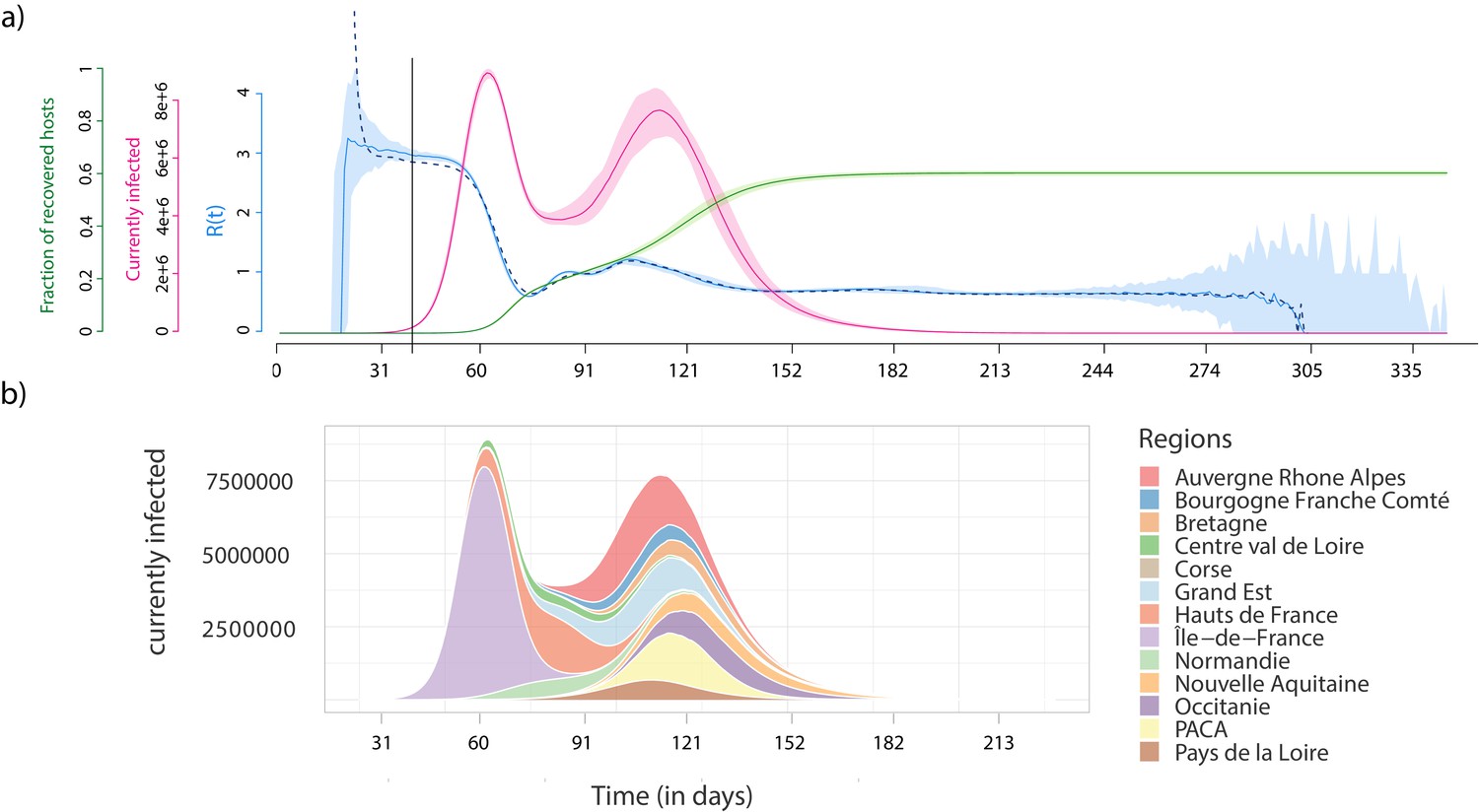
Epidemiological dynamics at the national (a) and regional (b) level.
(a) The daily prevalence (the number of infected individuals) is in red, the temporal reproduction number () in blue, and the cumulative number of recovered individuals in green. Shaded areas show the 95% sample quantiles of 100 stochastic simulations. The dashed line shows the median calculated on the case incidence data. (b) Each colour shows the prevalence in a French region.
The national prevalence data uncovers a bimodal structure of the epidemic, which can be understood by moving to the regional scale (Figure 2b). The first peak corresponds to the spread in the region where the outbreak emerges (here the Ile-de-France), whereas the second corresponds to the sum of the epidemic peaks in the other regions. This bimodal structure is particularly pronounced because of the high population density in the region of origin of the outbreak (Ile-de-France), but it is a direct consequence of the detailed geographical information in the simulation platform. As expected, in a well-mixed setting the parameters used for the transmission model yield a single peak (Figure 2—figure supplement 1).
The resolution of the Epidemap simulations allows us to perform analyses at the district level (see Videos 1 and 2). In Figure 3a, we show that the date of onset of the epidemic in an area strongly depends on its distance from the origin (here assumed to be Paris). Furthermore, there is an additional effect of density such that denser areas are infected first. Interestingly, at the departmental level, these trends are not significant, further showing the importance of a fine-grain simulation level. Furthermore, the total proportion of inhabitants of a district who have been infected at the end of the epidemic strongly increases with density. The pandemic propagation velocity also increases with time. This can be explained by the fact that, when incidence is high, long-distance dispersion events are not rare anymore, which biases the mean distance of contamination towards higher values. For densely populated districts (Figure 3b), this proportion converges towards the mean-field prediction from well-mixed models mentioned above (Kermack and McKendrick, 1927). However, if the population density is low, this proportion is more variable showing the limit of classical assumptions.

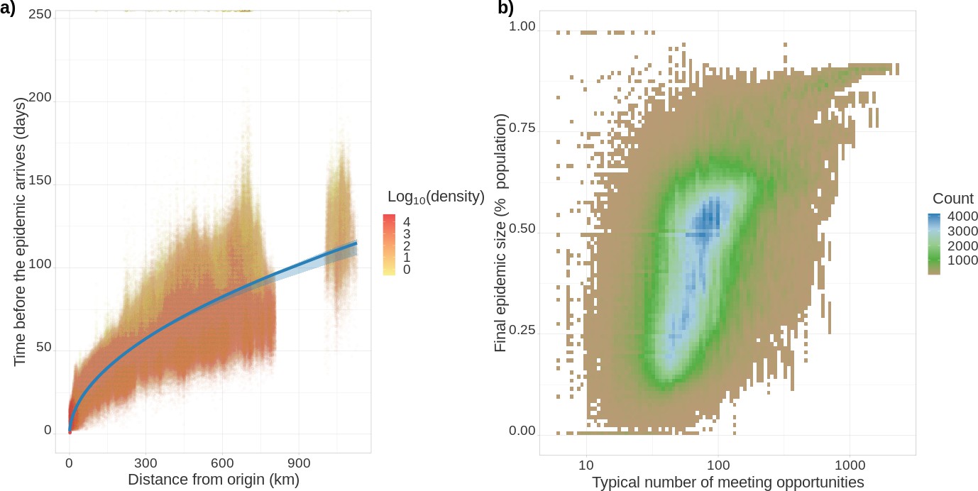
Epidemic arrival date and size at the district level.
(a) Effect of the distance from the epicentre on the number of days until the epidemic begins in a district. The colour indicates the population density in the district (number of inhabitants divided by the district’s surface). (b) District final epidemic size as a function of the characteristic distance between two individuals normalised by the average dispersal distance. The latter is computed as , where is the log-normal distribution of daily individual covered distance. Both panels show the value for 35,234 French districts and 100 stochastic simulations.
Density of residents in ICU throughout an uncontrolled epidemic.
The top panel shows the value at a fine geographical scale (French ‘canton’) and the bottom panel shows the total density at the national level along with the corresponding temporal reproduction number ().
Density of infected people / 100 k residents for an uncontrolled epidemic.
The top panel shows the value at a fine geographical scale (French ‘canton’) and the bottom panel shows the total density at the national level along with the corresponding temporalreproduction number (R(t)).
The individual-based nature of our simulations allows us to follow transmission chains (Video 3), which has direct applications. For instance, we can count, at the end of each infection, how many secondary infections were caused. The distribution of these individual reproduction numbers is particularly important in the context of emerging epidemics because the more disperse, the more the spread relies on super-spreading events (Lloyd-Smith et al., 2005). Early in the epidemic, the distribution is tightly centred around the R0 value (Figure 4a). As the epidemic unfolds, the distribution changes with a mode that decreases towards 0, and a wider dispersal. This pattern can be formalised by assuming that the distribution of individual reproduction numbers follows a negative binomial distribution (Lloyd-Smith et al., 2005). In Figure 4b, we show that the mean of this distribution (in blue) follows the pattern estimated in Figure 2a. The dispersal parameter () indicates that super-spreading events reach a peak at the end of the first national epidemic wave. During the end of the epidemic, stochasticity is strong but there is a general trend towards a decrease in super-spreading events. Note that in these simulations we do not introduce host heterogeneity, which means we only capture the dimension of superspreading that originates from spatial heterogeneity. This is already sufficient to show that studies attempting to quantify the importance of superspreading events should account for the stage of the epidemic they analyse.
Complete transmission chains colored by chain length of an uncontrolled epidemic.

Individual reproduction number dynamics.
(a) Distribution obtained over the whole population on 4 different days post outbreak. (b) Daily variation of the mean (in blue) and dispersion (in orange) of the distribution of individual reproduction numbers, which is assumed to follow a Negative Binomial distribution (Lloyd-Smith et al., 2005). Shaded areas show the 95% CI.
Finally, we focused so far on the infection spread but by adding a clinical part to the infection model, and therefore additional parameters (Table 3), we can also capture the hospital epidemic wave dynamics. For instance, Video 1 shows the detailed geographical dynamics of the density of residents in ICU. As expected in the case of SARS-CoV-2, where clinical dynamics have little effect on transmission dynamics due to the life-history of the infection (see the Materials and methods), these dynamics closely follow that of infection cases.
Discussion
Simulating the daily activity of millions of individuals at a build-level resolution with a realistic mobility model significantly improves our understanding of how epidemics unfold. Early stages appear to be consistent with stochastic and deterministic mean-field models. However, once local saturation effects cannot be neglected anymore, Epidemap reveals striking patterns with an unprecedented resolution. First, a two-waves epidemic pattern emerges at the French national level, which is largely driven by temporally shifted dynamics at the regional level. Second, we find that districts are affected by the epidemic depending on how far they are from the epicentre, but also depending on their density. The latter effect is absent at the departmental level, which illustrates the added value of a detailed geographical structure. Furthermore, as expected (Keeling, 1999), the simplistic estimate of the final epidemic size as a function of R0 does not apply at the national level. Conversely, this estimate does yield relevant results at the district level if the density is sufficiently high. Finally, being able to perform individual follow-ups allow us to see that super-spreading events become increasingly important as the epidemic unfolds, but that their role decreases as the importance of stochastic processes increase again at the end of the epidemic wave. In general, many insights can also the gained from the ability to follow individual trajectories and transmission chains (Video 3), and superspreading events.
Replacing these results in the broader context of infectious disease epidemiological modelling helps to better identify the originality of the approach. For instance, the link we identify between the final size of the epidemic in a district and its population density is not reported in the other ABS we discussed here, but appears quite strongly in SARS-CoV-2 data (Smith et al., 2021). Similarly, superspreading events are known to be an important target for public policies because they increase the risk of stochastic extinction but also to fuel the speed of spread of epidemics that do emerge (Lloyd-Smith et al., 2005). However, although field studies find that their importance may vary over the course of an epidemic (Lau et al., 2017), we are not aware of an in-depth analysis of these emerging trends using ABS. Note that since Epidemap can store transmission chains, which resemble infection phylogenies, we could further investigate the possibility to detect superspreading events using various kinds of data (Alizon, 2021).
Being able to perform such detailed simulations for so many agents at a national scale has to be traded-off against some simplifying assumptions. The major one is that individual movements are based on a distance kernel centered in their residency home. As shown by earlier work on influenza dynamics, although this assumption is relevant for France, it might be too simplistic for countries like the United States, where air traffic represents a greater proportion of the travels (Crépey and Barthélemy, 2007). A second limitation is that, because of the lack of relevant data, we assumed all individuals to have the same average behaviour, e.g. in terms of the number of buildings visited per day. This assumption was motivated by the will to develop a parsimonious study and not by a constraint of the Epidemap formalism. In fact, as mentioned in the Materials and methods, we already follow the age or the infectious status of the agents and could easily have mobility that depend on these parameters.
Focusing more specifically on the importance of individual age, there are several ways in which accounting for this data in the simulations could be of interest. First, we could investigate how patterns observed for some ‘childhood’ infectious diseases emerge in the simulations. Indeed, one possibility is that these are only due to children having specific mobility patterns, which could be modelled here by imposing that instead of visiting two buildings at random, they only visit the nearest school. Another possibility could be that explaining childhood infectious disease dynamics require children-specific patterns in the infection model, that is susceptibility to the infection and/or contagiousness. Finally, both could also be needed. By separating the mobility model and the infection model, and by introducing a high-resolution and realistic mobility model, Epidemap could yield original insights into such observed epidemiological patterns.
These results have immediate applications for public health. For instance, they allow authorities to derive a risk factor per district to help control an epidemic and prevent outbreaks. From an even more applied perspective, Epidemap can readily simulation hospitalisations by sending an individual to the nearest hospital, thereby allowing to anticipate the saturation of ICU at a detailed geographical level. In the context of the SARS-CoV-2 pandemic, this simulation platform can also be instrumental to optimise vaccine coverage but also compare the effect of specific Non-Pharmaceutical Intervention (NPI) (e.g. mask-wearing vs. stay-at-home requirements).
We focused here on respiratory infection similar to SARS-CoV-2 but an asset of this platform is its versatility. We already mentioned how it could be modified to investigate childhood respiratory infections. Simulating sexually transmitted infections could prove to be challenging with such a framework because these require to model partnerships and a fine-grain geographical resolution seems less crucial (Althaus et al., 2012). However, a more feasible extension could be the study of vector-borne diseases. Indeed, in Epidemap, the vector density could be directly informed by field data and used to implement infection risk. This could even be an opportunity to interact with the general public to benefit from local signalling of specific vectors (Pernat et al., 2021). Independently of the infection followed, Epidemap can then be used to explore a variety of control scenarios with high resolution at a national level.
Materials and methods
The approach used in Epidemap couples three models. The first model dispatches each agent to a building, depending on the national demographic distribution (INSEE, 2019) and the properties of the buildings (from OSM). The second model determines the buildings that each agent will daily visit and socials interactions with other agents located in the same distant buildings, and is based on that from Barbosa et al., 2018. Finally, the third model captures the life-history properties of the infectious disease in infected agents and is based on that from Sofonea et al., 2021.
Geographical structure
Request a detailed protocolWe use the freely available OSM database to extract all the points of interest for this study OSM. The accuracy of this database is partially high in France because the official national land registry (the ‘Cadastre’) database is merged into the OSM database. These databases are formatted in ASCII XML, with a size of approximately 80 GB for France.
OSM labels residential buildings specifically. We use the surface of these buildings and their geographical position to allocate each agent to a ‘home’ (residency) building. For the mobility model, we also include all the other types of buildings (e.g. hospitals, schools, airports, commercial centres, etc.), where agents can meet.
In our current simulations, the initial database size contains 4.1 108 nodes and 4.8 107 buildings that need to be pre-processed to compute additional characteristics such as building surface, usage, or geographical location, which can be reused in different simulations.
Demographic model
Request a detailed protocolThe Institut National de la Statistique et des Etudes Economiques (INSEE) publishes data with a high-level resolution of the distribution of the French population (INSEE, 2019). Here, we use the information about the full population in each city in 2016 to allocate agents to different locations. By combining this database and OSM’s, we can compute the number of residents in each building of each city.
More precisely, agents are allocated to buildings proportionally to their floor-surface projection. The number of agents in each building is given by the equation
where is the number of agent in the building , the number of residents in the city considered, the floor-surface projection of building , the total surface of all residential buildings in the city, the entire part of a number, and a scaling parameter such that .
The age of each agent is randomly generated and follows the age pyramid of the french residents, given by INSEE. In this study, age only affects the probability to develop several symptoms of the infection and, therefore, not the transmission dynamics of the epidemic.
Following the results from the study on individual movement patterns by Schneider et al., 2013, we assume that each person can visit two distant buildings per day (where it can meet other agents). Treating the number of visited buildings as a random variable would induce a smaller discretisation time and increase the computing time. Note that, as explained below, in some situations an agent visits less than two buildings per day.
To determine which building is visited by an agent, we first compute its distance from the home building as the crow flies. Mathematically, is assumed to follow a log-normal distribution, with . As shown in Table 1, this parameterisation yields results that are very consistent with the INSEE data (INSEE, 2016).
Lognormal randomly choosen values and INSEE statistic of the distance between residential and distant building.
Original datas (INSEE, 2016) and fitting.
INSEE statistic | ||
---|---|---|
lt10 km | 32.9% | 33.7% |
10 km km | 30.6% | 30.5% |
20 km km | 15.5% | 16.0% |
30 km km | 12.7% | 12.5% |
50 km km | 6.8% | 5.8% |
gt100 km | 1.5% | 1.5% |
We then randomly select the building visited by the individual among all the buildings located at a distance of the agent’s home (±50 m) using a weighting probability proportional to the floor-surface projection of the buildings. Therefore, larger buildings are visited by a higher amount of people than smaller ones. If no building is found at the randomly generated distance, the agent does not interact with any other agent for this movement round.
Every day, each agent can interact randomly and non-exclusively with other agents present in the same building at the same time. The maximum number of interactions is limited to 17 persons in a distant building and five in a residential building.
As indicated above, following our parsimonious approach, we assume that individual movements do not vary according to age or infection status.
Infection model
Request a detailed protocolEpidemap is versatile and can be adapted to simulate many infectious disease epidemics. Here, we simulate the case of a respiratory infection, focusing in particular on SARS-CoV-2. Given the life-cycle of the infection, schematised in Figure 5 we can separate the transmission and clinical dynamics because the latter has little to no effect on the former. Indeed, data shows that patients are typically hospitalised 2 weeks after infection. Of the secondary infections, 95% occur within the first 11 days post-infection. Furthermore, only a small fraction of the hosts are hospitalised (less than 1% in France O'Driscoll et al., 2021). The parameterisation was done using data from the French COVID-19 epidemic (Sofonea et al., 2021; Tables 2 and 3).

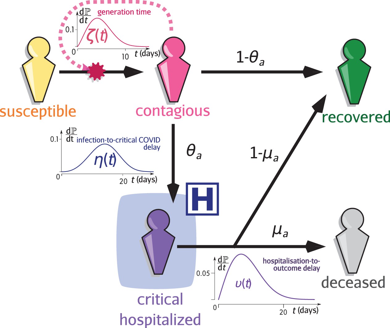
Infection model flow chart.
Susceptible individuals (yellow figurine), are exposed to viral transmission from contagious individuals (pink figurine). Once infected, a host is more or less contagious depending on the time since contamination according to distribution called the generation time (and usually parameterised using the empiric serial interval). A fraction , the value of which depends on the age of the host , will develop a critical infection and be admitted to a hospital (purple figurine) according to the complication delay distribution . The complementary fraction is assumed to recover with perfect and long-lasting immunity (green figurine). This compartment is also reachable after hospitalisation with the age-dependent probability , after the discharge delay distribution . The complementary fraction eventually dies from COVID-19. See Sofonea et al., 2021 for additional details.
Parameters used for the transmission model in the simulations.
LN stands for log-normal, We for Weibull.
Name | Description | Value | Reference |
---|---|---|---|
Number of agents (population size) | 6.6E7 | INSEE, 2019 | |
Number of buildings visited during the day (+ home) | 3 | Schneider et al., 2013 | |
Individual dispersal kernel distance | fit of INSEE, 2016 | ||
N1 | Maximum daily number of agent met (distant) | 17 | user-defined |
N2 | Maximum daily number of agent met (at home) | 5 | user-defined |
Contagiousness days after infection | Nishiura et al., 2020 | ||
Transmission probability per contact | Variant Technical group, 2021 |
Parameters used for the clinical progression of the infections in the simulations.
These parameters do not affect virus spread. LN stands for log-normal, We for Weibull.
Name | Description | Value | Reference |
---|---|---|---|
µ | Hospital mortality rate | 56% | Santé Publique France, 2020 |
ICU admission daily probability for a severely infected patient | Linton et al., 2020 | ||
ICU departure daily probability | Linton et al., 2020 | ||
Probability for a severely infected patient of age to die | Verity et al., 2020 |
For each interaction between a susceptible and an infected agent, we assume a constant probability of contamination (Variant Technical group, 2021) multiplied by normalised daily infectivity, or generation time, which follows a Weibull distribution with parameters and , with the number of day since contamination (Nishiura et al., 2020). We can simulate the effect of non-pharmaceutical interventions (e.g. mask-wearing) by decreasing this probability. Therefore, the transmission model only requires three parameters, two of which can be informed from contact-tracing data (Nishiura et al., 2020).
A fraction of infections, where is the age of the host, become critical (i.e. leading to intensive care unit (ICU) admission and/or death). These individuals have a daily probability to be hospitalised and then a daily probability to either recover or die, with probability and respectively. All recovered hosts are assumed to be immune to the infection until the end of the simulation.
Simulation specifications
Request a detailed protocolBecause of the strong heterogeneity in the first stages of the epidemic, we perform 100 simulations. To minimise the risk of early extinction of the outbreak, each simulation is seeded by infecting 15 individuals in a building at geographical coordinates 48.87732, 2.32993, which is in the area of Paris (a likely city in France for an introduction given its connectivity to the rest of the world).
The parameters used for these simulations are summarised in Table 2. For the type of infections considered, the clinical dynamics do not affect the transmission dynamics and, therefore, the parameters related to the clinical part of the infection are shown in a separate Table 3.
The computing code is written in Fortran 90 (F90) with Open Multi-Processing (OMP) approach to parallelise the computation and contains lines. A huge effort was made to reduce the memory print of the code, which runs with less than 64 GB Random Access Memory (RAM) for 6.6 107 agents. A full epidemic simulation, which represents approximately 300 days, is performed in 2 hr on a standard personal computer (12-cores AMD Ryzen 9). The statistics are written in ASCII format and the graphical outputs use the compressed Paraview format.
Comparisons with other platforms are indicative because each software has its own properties. For instance, as explained in the introduction, although most softwares do not have the same geographical resolution as Epidemap, some have more detailed social structures such as households. Furthermore, for many softwares, this information is not available. The recent OpenABM platform (Hinch et al., 2021) is very transparent about its computation times: takes 1.5 s a 2019 MacBookPro (2.4 GHz Quad-Core Intel Core i5) to simulate 1 day of epidemics for 1 million individuals. To perform our study (100 simulations of 66 million of agents during a year), the computing time would be ≈40 days instead of ≈8 days with Epidemap. Covasim (Kerr et al., 2021) would run faster (in approximately 1 day) but does not have spatial structure. In both cases, these estimates assume perfect scaling. Furthermore, the memory required can also raise some problems. For instance, the memory required to store the transmission chain data for the contact-tracing component of OpenABM is ≈3 kB per agent per epidemic week simulated. For one of our runs, that is the simulation of 66 million agents during one year, this would require more than 10 TB of RAM, which is clearly beyond the capabilities of a standard computer. Epidemap requires less than 64 GB for such a run. Covasim would require the same amount of RAM but for shorter simulations (100 days) and no spatial structure. Aleta et al., 2020 and Rockett et al., 2020 do not seem to provide indications regarding the computing speed of their framework.
Data availability
The raw data associated with the 100 simulations performed and the R scripts used to generate the figures are available from the Zenodo repository at https://zenodo.org/record/5542171 (results.zip).
-
ZenodoEmerging dynamics from high-resolution spatial numerical epidemics.https://doi.org/10.5281/zenodo.5542171
References
-
Agent based modelling and simulation tools: a review of the state-of-art softwareComputer Science Review 24:13–33.https://doi.org/10.1016/j.cosrev.2017.03.001
-
Transmission of Chlamydia trachomatis through sexual partnerships: a comparison between three individual-based models and empirical dataJournal of The Royal Society Interface 9:136–146.https://doi.org/10.1098/rsif.2011.0131
-
BookInfectious Diseases of Humans Dynamics and ControlOxford: Oxford University Press.https://doi.org/10.1001/jama.1992.03490230111047
-
Human mobility: Models and applicationsPhysics Reports 734:1–74.https://doi.org/10.1016/j.physrep.2018.01.001
-
Estimation in emerging epidemics: biases and remediesJournal of The Royal Society Interface 16:20180670.https://doi.org/10.1098/rsif.2018.0670
-
Detecting robust patterns in the spread of epidemics: a case study of influenza in the United States and FranceAmerican Journal of Epidemiology 166:1244–1251.https://doi.org/10.1093/aje/kwm266
-
(Meta)population dynamics of infectious diseasesTrends in Ecology & Evolution 12:395–399.https://doi.org/10.1016/S0169-5347(97)01174-9
-
OpenStreetMap: User-Generated Street MapsIEEE Pervasive Computing 7:12–18.https://doi.org/10.1109/MPRV.2008.80
-
WebsiteDe plus en plus de personnes travaillent en dehors de leur commune de résidenceBilan Démographique. Accessed October 29, 2021.
-
WebsitePopulations légales 2017. recensement de la population régions, départements, arrondissements, cantons et communesBilan Démographique. Accessed October 29, 2021.
-
WebsitePopulation totale par sexe et âge au 1er janvier 2020Bilan Démographique. Accessed October 29, 2021.
-
The effects of local spatial structure on epidemiological invasionsProceedings of the Royal Society of London. Series B: Biological Sciences 266:859–867.https://doi.org/10.1098/rspb.1999.0716
-
BookModeling Infectious Diseases in Humans and AnimalsPrinceton University Press.https://doi.org/10.2307/j.ctvcm4gk0
-
A contribution to the mathematical theory of epidemicsProceedings of the Royal Society of London 115:700–721.https://doi.org/10.1098/rspa.1927.0118
-
Covasim: An agent-based model of COVID-19 dynamics and interventionsPLOS Computational Biology 17:e1009149.https://doi.org/10.1371/journal.pcbi.1009149
-
Moment equations in spatial evolutionary ecologyJournal of Theoretical Biology 405:46–57.https://doi.org/10.1016/j.jtbi.2015.10.014
-
Serial interval of novel coronavirus (COVID-19) infectionsInternational Journal of Infectious Diseases 93:284–286.https://doi.org/10.1016/j.ijid.2020.02.060
-
Citizen science versus professional data collection: Comparison of approaches to mosquito monitoring in GermanyJournal of Applied Ecology 58:214–223.https://doi.org/10.1111/1365-2664.13767
-
BookCovid-19 : Point Épidémiologique Hebdomadaire Du 15 Mars 2020Santé Publique France.
-
Unravelling daily human mobility motifsJournal of The Royal Society Interface 10:20130246.https://doi.org/10.1098/rsif.2013.0246
-
Inferring R0 in emerging epidemics-the effect of common population structure is smallJournal of The Royal Society Interface 13:20160288.https://doi.org/10.1098/rsif.2016.0288
-
BookInvestigation of novel SARS-COV-2 variant: Variant of concern 202012/01 Technical Briefing 3Public Health England.
-
Estimates of the severity of coronavirus disease 2019: a model-based analysisThe Lancet Infectious Diseases 20:669–677.https://doi.org/10.1016/S1473-3099(20)30243-7
-
How generation intervals shape the relationship between growth rates and reproductive numbersProceedings of the Royal Society B: Biological Sciences 274:599–604.https://doi.org/10.1098/rspb.2006.3754
Decision letter
-
Talía MalagónReviewing Editor; McGill University, Canada
-
Eduardo FrancoSenior Editor; McGill University, Canada
In the interests of transparency, eLife publishes the most substantive revision requests and the accompanying author responses.
Acceptance summary:
This work presents a dynamic infectious disease transmission model using geospatial data to structure transmission, using SARS-CoV-2 transmission in France as an example. The model allows for the incorporation of fine grain spatial heterogeneity and a large number of simulated individuals, providing a computationally efficient alternative to traditional agent-based models and a more realistic geographical mixing structure than traditional compartmental model. The Epidemap framework has many potential uses for supporting infectious disease planning and response activities beyond the SARS-CoV-2. The work will be of interest to infectious disease modelers, epidemiologists, and public health decision-makers working in epidemic outbreak management.
Decision letter after peer review:
Thank you for submitting your article "Emerging dynamics from high-resolution spatial numerical epidemics" for consideration by eLife. Your article has been reviewed by 3 peer reviewers, one of whom is member of our Board of Reviewing Editors, and the evaluation has been overseen by a Senior Editor. The reviewers have opted to remain anonymous.
The reviewers have discussed their reviews with one another, and the Reviewing Editor has drafted this to help you prepare a revised submission.
Essential revisions:
1. The paper does not currently meet eLife's policy regarding Availability of Data, Software, and Research Materials. The revision should include material to meet this policy.
2. The paper should be reformatted using a more traditional structure to improve readability (Introduction, Methods, Results, Discussion).
3. Include further explanations and discussion regarding how age is integrated into the model, or how the model could be extended to include host heterogeneity by age.
4. Include further description and explanation of how the distance kernel and mobility kernel were modeled.
5. There is currently very little discussion on how the results of this study compare with results from previous traditional models. There should be more discussion on how this study fits into previous literature on this topic, including the citation of key previous papers that have examined issues of spatial heterogeneity.
6. Include more high-level details regarding the model structure from the appendix in the main text to help the reader understand the structure without having to refer to previously published papers. The reviewers provide some suggestions in their reviews for which elements could be included.
7. The paper currently includes specifications regarding the computational resources needed for this platform, but should also include further discussion on computational resources required by traditional compartmental and agent-based models to so that the reader can appreciate the difference. Further discussion on how model results and computational resources compare with traditional compartmental and agent-based models.
8. Further discussion around limitations of the tool, particularly in the case of application to other infections where distance alone may not sufficiently capture transmission patterns.
Reviewer #1:
In this work, the authors present an infectious disease transmission model using geospatial data to structure transmission. Their aim was to produce a stochastic agent-based model that integrates geographic structure and infection natural history with sufficient realism without being too computationally demanding. By integrating map and daily mobility information, the work shows that interesting infection dynamics may occur at different geographical levels when geographic structure is considered in the context of transmission. Models incorporating geographical information are likely to be increasingly valuable in the future, as the COVID-19 pandemic has highlighted the need to consider regional and local needs when implementing public health measures against a pandemic pathogen.
Some of the model strengths include the use of detailed geographical information, and a minimal number of parameters needed to inform the model. A wide range of natural history of infection models can potentially be integrated to represent different agents with different transmission and immunity profiles. Perhaps one of the weaknesses of the model is the lack of age stratification, which would increase the realism of the model and provide important epidemiological information from a public health perspective. Age has turned out to be an important variable in tracking the COVID-19 pandemic impact and public health response. While the authors mention the model tracks the age of participants, the parameters and behaviors of agents do not appear to depend on age. A further discussion of how this model could be extended to include more heterogeneity in the movement patterns of agents would be useful, and whether the inclusion of further complexity would substantially increase the computational burden of simulations. There is also no data presented regarding the hospitalization component of the model, which is briefly described but not explored.
I think one of the major contributions of this work is the illustration of how high-resolution geographical data can be integrated into infectious disease models. These methods are likely to be of high interest to other infectious disease modelers, and to public health experts working in epidemic outbreak management.
– The paper does not currently meet eLife's policy regarding Availability of Data, Software, and Research Materials (https://submit.elifesciences.org/html/eLife_author_instructions.html#policies). I can appreciate that the dataset generated by the model is too large to be made available in free data repositories. However, this does not preclude increasing the reproducibility and availability of the data. In cases where the data can't be made available, it is up to the authors to explain in the manuscript the restrictions on the dataset or materials and why it is not possible to give public access. They must also provide a description of the steps others can follow to request access to the data or materials if they are interested. It is also good practice to provide access to data and materials for which the constraints do not apply. For example, what I have seen in similar cases with large or un-shareable datasets is that the authors would provide the necessary code to reproduce figures and tables in the manuscript with a smaller simulated dataset. Often also the dataset can be broken down into smaller datasets of the processed data necessary to reproduce each figure. While Figure 3 might be problematic due to the large number of observations, Figures 2 and 4 would likely be amenable to this as each panel appears to only display the results from a couple hundred data points. I suggest the authors consider this option. This should all be included in the data availability statement as well.
– Please further discuss how the model could be built on to add further demographic stratifications such as age to natural history/daily mobility patterns and interactions between agents. Would the addition of further stratifications severely affect the computational burden?
– The authors mention a parameter regarding hospitalization probability and severity of infection; however, these parameters are not included in the table of parameters in the appendix. It would seem to me there are more than 6 parameters in the model then. It is unclear why these parameters were added, as they are not explored in the results or mentioned very much in the text. Some more discussion or results regarding this component of the model would be warranted.
– There is little discussion of other models which have implemented geographical structure, and how this model compares with those. I am not very familiar with this literature, but I find it hard to believe that none have tried to implement some geographical component. Some more discussion on how this approach is innovative or different compared to what has been done in the past would be useful.
– It would be useful to include the names of the scientific papers cited in the reference list, most of these are not full references.
Reviewer #2:
This work provides a new general tool for studying the chains and patterns of transmission of infectious diseases. It addresses the limitations of mathematical models and the Agent-Based Simulation platforms in public health by using High-Performance Computing techniques, high-resolution spatial data, and complex mobile models. Based on the results of 100 stochastic simulations, the basic reproduction number, the duration of the disease and the final total epidemic size were obtained at the national level, which shows the importance of the geographical structure. Meanwhile, the influence of the distance from origin and the density of the region on the epidemic was shown at the district level. Finally, this paper also shows that the importance of super-spreading events varies according to the stage of the epidemic.
1. In the Introduction part, the authors mentioned some work on COVID-19 based on mathematical modelling. However, some existed work are not well respected. Please see some papers: Short-term predictions and prevention strategies for COVID-19: A model-based study, Applied Mathematics and Computation, 2021; Analysis of COVID-19 transmission in Shanxi Province with discrete time imported cases, MBE, 2020; An investigation of transmission control measures during the first 50 days of the COVID-19 epidemic in China, Science, 2020; Transmission dynamics of COVID-19 in Wuhan, China: effects of lockdown and medical resources, Nonlinear Dynamics, 2020.
2. For readability, please give a brief description and introduction of a distance kernel and a mobility kernel mentioned in line 52 in the text.
3. In line 55, the author mentioned that the simulation tracked the age of the individual, but this was not further described and shown in the text, as well as the description of the relevant simulation result. Given the importance of age to COVID-19, further research on age should be conducted.
4. This paper demonstrates the power and flexibility of the Epidemap platform through the application of COVID-19 in France. However, all the results obtained in the paper are obtained through numerical simulation, the authors should compare them with the real data at the national and district level of France to further prove the rationality, practical application and authenticity of this method.
Reviewer #3:
Thomine et al., have a developed a new tool for modeling infectious diseases which can consider fine grain geographic movements of tens of millions of individual agents (simulated persons), thereby enabling more realistic simulations (compared to SIR models) without the excessive computational demands required by traditional agent-based modeling approaches. Impressively, this tool, Epidemap, was able to simulate one year of daily interactions and epidemic growth trajectories for the entire population France (approximately 65 million people) in less than two hours using a standard high performance computer.
The authors present the example of an uncontrolled SARS-CoV-2 epidemic in France and identified spatio-temporal differences in disease and transmission dynamics that would not be discernable using naïve SIR modeling approaches and would be extremely computationally demand to complete using traditional ABM methods. These observations included a distinct bimodal pattern, in which each peak was comprised of different localities; a strong correlation between the timing of the epidemic peak in different regions and its distance from the point of epidemic origin; important differences in disease dynamics based on population density; and unique insights regarding secondary attack rates measured at the individual level (i.e., the reproductive number). These observations could support evidence-informed targeting of public health measures to optimize the impact of mitigation measures and support health care planning. This tool could also have great applicability to the study of other respiratory infections, particularly if additional features further enhancing the realism of the simulations, such as assigning children to schools, can be added without substantially increasing computational demands. The visual component of this tool is an especially nice feature, which could greatly support knowledge translation activities with decision-makers and planners.
The rationale for the development of this tool is clear (and important), the conclusions of this manuscript are supported by the data, and the paper is well-written. The included figures, particularly Figure 1, are very easy to follow and nicely display the key take-away messages.
The methods section could benefit from additional details to better able the reader to understand the development of this tool, specifically:
1) Please provide adequate details regarding the fundamentals of this approach in the main manuscript text. The material provided in S1 Supplementary Methods is critical to understanding this tool, particularly the summary statement regarding the three specific models. For example, the manuscript refers to the epidemiological model, but the reader must refer to a reference to learn more. Providing some high-level details regrading the model and the hospital data (including how they were used to parametrize the model) would be helpful. Similarly, it is stated that the disease progression model follows that of reference 10 – having a figure included in the manuscript would be helpful – and the daily reproduction numbers were based on a method from 18 – a brief description would be appreciated.
2) How do these findings compare to traditional SIR or ABM models? Understandably, it may be too computationally demanding to run a traditional ABM for the entire population of France and would likely be out of scope for this study. For context, it would be useful to provide an estimate of the time and computational resources demanded by traditional approaches. If running these other models are possible, a comparison of the insights provided across these 3 methods would be highly valuable – particularly if there are large differences.
3) The probability of encounters is based only on distance. As the authors state, this assumption may not hold for other countries (e.g. the US where air travel is more important). This assumption may also not hold for other infections. For example, the transmission dynamics of pediatric respiratory viruses are more influenced by neighbourhood-level patterns of movement – whereas diseases of adults are more heavily influenced by larger-scale geographic patterns. Please provide the reader with more context around this limitation.
– Abstract: I'm not sure if "computational-efficient" is grammatically correct – suggested revision: computationally efficient.
– The introduction section could be strengthened by first introducing the idea of a mathematical model – and their uses – before discussing their limitations. Could you provide the reader with an explicit example of where these models have failed because they did not contain the features of an ABM (or Epidemap)? There are several examples from the COVID-19 pandemic and Ebola epidemics that readers would be familiar with and would allow them to immediately appreciate the importance of the current work.
– Introduction: You state that SIR models ignore spatial contact patterns. Though the naïve SIR model does, most SIR models are age-structured and include some sort of contact matrix (e.g. POLYMOD). Suggest rewording to "and oversimplifies contact patterns".
– Regarding the following statement: "A third limit resides in the way geographic structure is implemented into the simulation (but see (7))." Please clarify what is meant without the reader referring to a reference.
– Such a model is likely only relevant to the study of respiratory viruses, this should be stated as a limitation – or, if modifications can be made to enable the study of other infectious diseases (e.g. STIs), this should be highlighted as a strength of Epidemap.
– The readability of the manuscript would also benefit from a more traditional structure, i.e., sub-headers in the abstract and main text for background, methods, results, and discussion. Similarly, the funding statement is provided as reference. This, along with a conflict of interest statement, should be explicitly provided in-text.
– In the supplement, you refer to the spread of COVID-19. Recommended revision: SARS-CoV-2.
– To enhance the clarity of Figure 2, it would be helpful to line-up the x-axes of (a) and (b).
Specific aspects of the methodology that are not clear from the manuscript or supplemental:
– The justification for some modeling choices has not been provided and it is not clear what impact, if any, this would have had on the results. Namely, what was the rationale for initializing the model with 15 infected individuals in Paris and aligning the axis for Figure 2 based a value of 700 ICU beds. Assumedly, the choice for Paris is due to this being the most likely place for importation, but this is not clear. The choices for the other two values appears arbitrary.
– It is not clear how the interaction model accounts for household and school/workplace encounters. For example, are these included in the random movement or separately? Does the risk of transmission differ in these contexts? These dynamics would be quite different than a random encounter at, for example, the grocery store. Similarly, can transmission occur within hospitals?
– The age of contacts is recorded, but it is not clear how/if this information is incorporated into the simulation; e.g. differences in disease severity profiles on the basis of age.
– How were the point estimates and 95% CI calculated?
https://doi.org/10.7554/eLife.71417.sa1Author response
Essential revisions:
1. The paper does not currently meet eLife's policy regarding Availability of Data, Software, and Research Materials. The revision should include material to meet this policy.
We posted on the Zenodo server the raw outputs of the simulation data (ASCII format), as well as the R scripts used to generate the figures.
The availability of the data and scripts is now mentioned in the manuscript.
2. The paper should be reformatted using a more traditional structure to improve readability (Introduction, Methods, Results, Discussion).
We now highlight the article structure and included a clear Methods section.
3. Include further explanations and discussion regarding how age is integrated into the model, or how the model could be extended to include host heterogeneity by age.
This is an individual-based simulation so each individual has an age, which is randomly chosen based on the French demographics data from INSEE (the French statistics institute). In the simulation, the age only affects the clinical part of the model, i.e. the probability to develop severe symptoms and be hospitalised. There are several ways in which age could be included in the model. One possibility could be to implement realistic household structures using existing data. Furthermore, regarding the daily mobility patterns, we could simulate school attendance by imposing that during the week days all children visit the nearest school (a piece of information that is available through the OpenStreetMaps/OSM data). Similarly, for older individuals, we could simulate residency in age care facilities, although this data may require more effort to be extracted from OSM. These examples were not implemented in these first simulations to avoid increasing the number of free parameters but EPIDEMAP does offers many possibilities to investigate the role of age in epidemic spread and simulate control scenarios.
We now mention some of the scenarios that could be explored in EPIDEMAP using the age structure already implemented.
4. Include further description and explanation of how the distance kernel and mobility kernel were modeled.
We apologize for putting all the details about the distance kernel in the Appendix. As we now detail in the Methods section, all individuals are assigned to an OSM building (their ‘home’). Each day, they can visit 2 additional buildings and this is where the distance kernel matters. These buildings are chosen at random on a circle the radius of which is drawn at random in a lognormal distribution. If more than one building intersects with the circle, we draw a building at random. If there is no building on the circle, this movement is cancelled.
We now discuss the distance kernel in the new Methods section.
5. There is currently very little discussion on how the results of this study compare with results from previous traditional models. There should be more discussion on how this study fits into previous literature on this topic, including the citation of key previous papers that have examined issues of spatial heterogeneity.
This is a delicate issue because there is a wealth of individual based models (IBM) but very few nationwide models are performed with a realistic geographical mapping. Indeed, spatially explicit individual-based model tend to have a higher level of granularity (e.g. with cells or districts in which individuals interact but where spatial structure does not matter). There are some exception, such as https://link.springer.com/article/10.1186/1471-2334-11-115
We now discuss in more details studies that investigated spatial heterogeneity and how our results on spatial epidemic spread relate to these.
6. Include more high-level details regarding the model structure from the appendix in the main text to help the reader understand the structure without having to refer to previously published papers. The reviewers provide some suggestions in their reviews for which elements could be included.
All the technical descriptions of the model were in the Appendix, which we agree was not ideal for readers who want to know more about the specificity of our simulator.
We added a Methods section to the main text of the manuscript.
7. The paper currently includes specifications regarding the computational resources needed for this platform, but should also include further discussion on computational resources required by traditional compartmental and agent-based models to so that the reader can appreciate the difference. Further discussion on how model results and computational resources compare with traditional compartmental and agent-based models.
In short, we are not aware of any existing individual based model that could handle so many individuals (66 million) in a spatially-explicit context on a similar (regular) desktop. For example, according to its specifications, the recent platform openABM takes 1.5s on a 2019 MacBookPro (2.4GHz QuadCore Intel Core i5) to simulate 1 days of epidemics for 1 million individuals. https://doi.org/10. 1371/journal.pcbi.1009146 It would therefore take 10 hours to simulate one of our runs (and without spatially explicit setting), assuming a perfect-scaling of their approach, where Epidemap took less than 2 hours. Furthermore, their approach requires «3kB per agent for tracing storage purposes for a 7 days pandemic. One simulation equivalent to ours would therefore require more than 10TB of RAM with this platform, which is clearly beyond the capabilities of a standard computer, where Epidemap needs less than 64 GB. Importantly, openABM has features that are not yet implemented in Epidemap, such as contact tracing and these may require additional memory. Furterhmore, their authors published these specifications, which is not the case of many simulators.
At the end of the Methods section, now compare more explicitly our computing power to more traditional agent-based models, while also pointing out that other models have some properties that are not (yet) included in Epidemap.
8. Further discussion around limitations of the tool, particularly in the case of application to other infections where distance alone may not sufficiently capture transmission patterns.
We indeed assumed that transmission occurs upon daily contacts, which better corresponds to respiratory infections. Simulating the spread of infections with other transmission routes could indeed be challenging. For instance, modelling sexual transmission would require to simulate partnerships in a more detailed way (see e.g. https://royalsocietypublishing.org/doi/full/10.1098/ rsif.2011.0131). Similarly, epidemics from vector-borne diseases would likely require an additional layer to simulate the vector demographics. However, would represent interesting future extensions for Epidemap, especially the vector-borne transmission mode.
We now better stress that the current implementation of the model is better suited to respiratory infections and discuss potential extensions to infections with different transmission routes.
Reviewer #1:
In this work, the authors present an infectious disease transmission model using geospatial data to structure transmission. Their aim was to produce a stochastic agent-based model that integrates geographic structure and infection natural history with sufficient realism without being too computationally demanding. By integrating map and daily mobility information, the work shows that interesting infection dynamics may occur at different geographical levels when geographic structure is considered in the context of transmission. Models incorporating geographical information are likely to be increasingly valuable in the future, as the COVID-19 pandemic has highlighted the need to consider regional and local needs when implementing public health measures against a pandemic pathogen.
Some of the model strengths include the use of detailed geographical information, and a minimal number of parameters needed to inform the model. A wide range of natural history of infection models can potentially be integrated to represent different agents with different transmission and immunity profiles. Perhaps one of the weaknesses of the model is the lack of age stratification, which would increase the realism of the model and provide important epidemiological information from a public health perspective. Age has turned out to be an important variable in tracking the COVID-19 pandemic impact and public health response. While the authors mention the model tracks the age of participants, the parameters and behaviors of agents do not appear to depend on age. A further discussion of how this model could be extended to include more heterogeneity in the movement patterns of agents would be useful, and whether the inclusion of further complexity would substantially increase the computational burden of simulations. There is also no data presented regarding the hospitalization component of the model, which is briefly described but not explored.
I think one of the major contributions of this work is the illustration of how high-resolution geographical data can be integrated into infectious disease models. These methods are likely to be of high interest to other infectious disease modelers, and to public health experts working in epidemic outbreak management.
Thank you for the positive assessment of our work!
Regarding the age structure, we apologise for the lack of clarity (which is probably due to the fact that most of the model details were in the Appendix). Indeed, the age stratification was already implemented (an individual is currently defined by her/his home building and her/his age). The age also affects the probability to develop a severe infection in the model (which is not shown in the model for focusing reasons). What we did not yet implement is a differential behaviour based on age, e.g. the fact that children attend school, or the fact that older people visit less buildings per day that younger people. As indicated to the Editor, these variations can readily be added but they also require solid data to avoid an inflation in the number of free parameters in the model.
We clarified the current role of individual age in the model.
We now discuss perspectives regarding heterogeneity in individual behaviour, especially depending on their age.
– The paper does not currently meet eLife's policy regarding Availability of Data, Software, and Research Materials (https://submit.elifesciences.org/html/eLife_author_instructions.html#policies). I can appreciate that the dataset generated by the model is too large to be made available in free data repositories. However, this does not preclude increasing the reproducibility and availability of the data. In cases where the data can't be made available, it is up to the authors to explain in the manuscript the restrictions on the dataset or materials and why it is not possible to give public access. They must also provide a description of the steps others can follow to request access to the data or materials if they are interested. It is also good practice to provide access to data and materials for which the constraints do not apply. For example, what I have seen in similar cases with large or un-shareable datasets is that the authors would provide the necessary code to reproduce figures and tables in the manuscript with a smaller simulated dataset. Often also the dataset can be broken down into smaller datasets of the processed data necessary to reproduce each figure. While Figure 3 might be problematic due to the large number of observations, Figures 2 and 4 would likely be amenable to this as each panel appears to only display the results from a couple hundred data points. I suggest the authors consider this option. This should all be included in the data availability statement as well.
As indicated in our response to the Editor, we posted the raw data on Zenodo, as well as the data and scripts used to generate the figures.
– Please further discuss how the model could be built on to add further demographic stratifications such as age to natural history/daily mobility patterns and interactions between agents. Would the addition of further stratifications severely affect the computational burden?
We do not expect additional stratification to affect computational burden if the traits involved are already implemented. The main risk for this study is the paramterisation issue. For instance, as we show for superspreading events, even without factoring these in explicitly in the model, they partly emerge from the simulations. Therefore, forcing a stratification or a heterogeneity without rich data may lead to an over-parameterisation of the model. As indicated in our response to the Editor, one of the most interesting extensions, which could be supported with data, is the household structure. This would naturally lead to additional age-stratification. Differences in behaviour could then be added on top of this.
We now discuss the main difficulty to add details to the model (which has more to do with the risk of over-parameterising the model) and which extensions are the most promising.
– The authors mention a parameter regarding hospitalization probability and severity of infection; however, these parameters are not included in the table of parameters in the appendix. It would seem to me there are more than 6 parameters in the model then. It is unclear why these parameters were added, as they are not explored in the results or mentioned very much in the text. Some more discussion or results regarding this component of the model would be warranted.
The model was developed in the context of the COVID-19 epidemic in France, and it does include a clinical component. The reviewer is entirely correct that the hospital (and mortality) component require additional parameters. However, these do not affect the results shown since, in the case of COVID-19, the hospital side of the epidemic has little effect on the spread of the infection in the general population (a small fraction is hospitalised and severe cases are admitted into hospitals 14 days after infection on average, whereas after 11 days, more than 95% of the secondary infections have already occurred). Overall, the three parameters related to the infection model that are required for the transmission model are the probability of transmission per contact and the two parameters capturing the serial interval distribution.
We now specify that the hospital and mortality extension of the model require additional parameters and add a second table showing the parameters related to this more clinical part of the model. We also added a video showing the number of hospital admission in France over the course of the simulation.
– There is little discussion of other models which have implemented geographical structure, and how this model compares with those. I am not very familiar with this literature, but I find it hard to believe that none have tried to implement some geographical component. Some more discussion on how this approach is innovative or different compared to what has been done in the past would be useful.
As indicated above, relatively few individual based model include detailed geographical structure (especially at a national level). In most models, this structure is discretised into subunits and a metapopulation approach is applied where individuals interact within their unit/population and migrate between populations. Some frameworks allow to perform similar simulations with high spatial resolution, e.g. the GAMA platform, but they tend to cover smaller geographical areas (partly to limit the number of individuals).
We now discuss more extensively the literature on explicit geographical structure in individual based models in the Introduction with a focus on recent COVID-19 models.
– It would be useful to include the names of the scientific papers cited in the reference list, most of these are not full references.
The initial reference style used was indeed poorly informative. We now switched to eLife’s LATEX template.
Reviewer #2:
This work provides a new general tool for studying the chains and patterns of transmission of infectious diseases. It addresses the limitations of mathematical models and the Agent-Based Simulation platforms in public health by using High-Performance Computing techniques, high-resolution spatial data, and complex mobile models. Based on the results of 100 stochastic simulations, the basic reproduction number, the duration of the disease and the final total epidemic size were obtained at the national level, which shows the importance of the geographical structure. Meanwhile, the influence of the distance from origin and the density of the region on the epidemic was shown at the district level. Finally, this paper also shows that the importance of super-spreading events varies according to the stage of the epidemic.
Thank you for this accurate summary.
1. In the Introduction part, the authors mentioned some work on COVID-19 based on mathematical modelling. However, some existed work are not well respected. Please see some papers: Short-term predictions and prevention strategies for COVID-19: A model-based study, Applied Mathematics and Computation, 2021; Analysis of COVID-19 transmission in Shanxi Province with discrete time imported cases, MBE, 2020; An investigation of transmission control measures during the first 50 days of the COVID-19 epidemic in China, Science, 2020; Transmission dynamics of COVID-19 in Wuhan, China: effects of lockdown and medical resources, Nonlinear Dynamics, 2020.
Searching the keywords "mathematical + modelling + COVID-19" in the Web of Science led to 2,765 references and reviewing all of these is clearly beyond the scope of this study. Furthermore, we are unsure as to why the reviewer singled out these studies because none of these correspond to individual based models.
1. Nadim et al., (2021, Applied Mathematics and Computation) develop a very basic ODE model which is very similar to dozens of models published before,
2. Li et al., (2020, Mathematical Biosciences and Engineering) use a simpler discrete-time model to analyse the cumulative number of cases in China, a strong limitation being that cumulative number of cases is easier to fit than incidence time series,
3. Tian et al., (2020, Science) analyse some valuable data but from a modelling perspective, all they seem to be implementing is a mean field SEIR model,
4. Sun et al. (2020, Nonlinear Dynamics) is very similar to the model by Nadim et al. (a basic ODE model with 5 compartments) and, as Li et al., is used to fit cumulative incidences.
We clarified the manuscript to underline that the originality of this study is not about COVID-19 epidemiological modelling and that there are few individual based studies that feature explicit geographical location.
2. For readability, please give a brief description and introduction of a distance kernel and a mobility kernel mentioned in line 52 in the text.
As indicated above, we apologise for the lack of clarity and the fact that most of the Methods we in Appendix.
We added a Methods section to describe the technical details of the simulations.
3. In line 55, the author mentioned that the simulation tracked the age of the individual, but this was not further described and shown in the text, as well as the description of the relevant simulation result. Given the importance of age to COVID-19, further research on age should be conducted.
This point was also raised by the other reviewer. Age is indeed an important factor regarding the infection fatality ratio of many respiratory infections. It was already included in the simulations but we indeed chose not to underline the results regarding mortality and hospital admissions to focus on the simulator itself.
We clarified the role of age and now show the hospital admission data and the mortality data in the Appendix.
4. This paper demonstrates the power and flexibility of the Epidemap platform through the application of COVID-19 in France. However, all the results obtained in the paper are obtained through numerical simulation, the authors should compare them with the real data at the national and district level of France to further prove the rationality, practical application and authenticity of this method.
The goal of the simulator is not to recreate the true epidemic, which would require to factor in all the public health and political decisions. Furthermore, the intensity of the computations and the level of detail make it also impractical to use such a simulator for parameter estimation (simpler compartmental models are more suited to analyse past data). The goal of a detailed simulator as EPIDEMAP is to analyse different scenarios using the most parsimonious approach (besides the hospital side of the epidemics, our model only requires 6 parameters) to simulate epidemics. Furthermore, our analyses on the resulting patterns indicate high level of biological realism, as illustrated for instance by the distribution of ….
We clarified at the end of the Introduction that the goal of EPIDEMAP is not to simulate the epidemic as it occurred or to perform statistical parameter estimation. We explain that it is a tool to explore epidemic scenarios with a high level of resolution.
Reviewer #3:
Thomine et al., have a developed a new tool for modeling infectious diseases which can consider fine grain geographic movements of tens of millions of individual agents (simulated persons), thereby enabling more realistic simulations (compared to SIR models) without the excessive computational demands required by traditional agent-based modeling approaches. Impressively, this tool, Epidemap, was able to simulate one year of daily interactions and epidemic growth trajectories for the entire population France (approximately 65 million people) in less than two hours using a standard high performance computer.
The authors present the example of an uncontrolled SARS-CoV-2 epidemic in France and identified spatio-temporal differences in disease and transmission dynamics that would not be discernable using naïve SIR modeling approaches and would be extremely computationally demand to complete using traditional ABM methods. These observations included a distinct bimodal pattern, in which each peak was comprised of different localities; a strong correlation between the timing of the epidemic peak in different regions and its distance from the point of epidemic origin; important differences in disease dynamics based on population density; and unique insights regarding secondary attack rates measured at the individual level (i.e., the reproductive number). These observations could support evidence-informed targeting of public health measures to optimize the impact of mitigation measures and support health care planning. This tool could also have great applicability to the study of other respiratory infections, particularly if additional features further enhancing the realism of the simulations, such as assigning children to schools, can be added without substantially increasing computational demands. The visual component of this tool is an especially nice feature, which could greatly support knowledge translation activities with decision-makers and planners.
The rationale for the development of this tool is clear (and important), the conclusions of this manuscript are supported by the data, and the paper is well-written. The included figures, particularly Figure 1, are very easy to follow and nicely display the key take-away messages.
Many thanks for this very detailed and enthusiastic presentation of our work!
The methods section could benefit from additional details to better able the reader to understand the development of this tool, specifically:
1) Please provide adequate details regarding the fundamentals of this approach in the main manuscript text. The material provided in S1 Supplementary Methods is critical to understanding this tool, particularly the summary statement regarding the three specific models. For example, the manuscript refers to the epidemiological model, but the reader must refer to a reference to learn more. Providing some high-level details regrading the model and the hospital data (including how they were used to parametrize the model) would be helpful. Similarly, it is stated that the disease progression model follows that of reference 10 – having a figure included in the manuscript would be helpful – and the daily reproduction numbers were based on a method from 18 – a brief description would be appreciated.
As indicated in our replies to the other reviewers, we heartily acknowledge that the detailed methods were difficult to follow being mostly in the Appendix. In the new methods section we added to the main text, we further describe the model used for disease progression. Furthermore, we also show the corresponding outputs for hospital admission data and mortality data in the Appendix.
We added a new Methods section, in which we describe the disease progression model and the tools used to estimate the reproduction number.
2) How do these findings compare to traditional SIR or ABM models? Understandably, it may be too computationally demanding to run a traditional ABM for the entire population of France and would likely be out of scope for this study. For context, it would be useful to provide an estimate of the time and computational resources demanded by traditional approaches. If running these other models are possible, a comparison of the insights provided across these 3 methods would be highly valuable – particularly if there are large differences.
If the reviewers’ suggestion is to compare our model to a classical ABM with the whole French population without spatial structure, the answer is each because this should yield the same results as model based on the equations used to simulate disease progression and transmission. Such a framework is already implemented in the COVIDSIM model (Sofonea et al., 2021 Epidemics). The only thing to do is to have the same basic reproduction numbers (R0) in EPIDEMAP and in this model. In the Appendix, we now show the dynamics of the daily case incidence for the transmission model without spatial structure and for the EPIDEMAP simulations.
We added a figure in the Appendix (Supplementary Figure S1) to show the epidemiological dynamics using the same parameters but in a setting without spatial structure.
3) The probability of encounters is based only on distance. As the authors state, this assumption may not hold for other countries (e.g. the US where air travel is more important). This assumption may also not hold for other infections. For example, the transmission dynamics of pediatric respiratory viruses are more influenced by neighbourhood-level patterns of movement – whereas diseases of adults are more heavily influenced by larger-scale geographic patterns. Please provide the reader with more context around this limitation.
We completely agree with this limitation. In the current simulations, we assume that host age does not affect susceptibility to the infection or contagiousness. Adding these effects would be very valuable to focus on specific infections. It would, however, require to improve some features of the model, especially the household structure and potentially also the mobility patterns (by having children attending schools). Such an implementation could be particularly interesting because it might uncover interactions between age-based differences in spatial/mobility patterns and in biology (sensitivity to infection and contagiousness).
When discussing potential extensions of the model to include household structure and age-based mobility patterns, we now explain how this could be particularly useful to better understand infections that spread differently across age groups.
– Abstract: I'm not sure if "computational-efficient" is grammatically correct – suggested revision: computationally efficient.
We made the changes.
– The introduction section could be strengthened by first introducing the idea of a mathematical model – and their uses – before discussing their limitations. Could you provide the reader with an explicit example of where these models have failed because they did not contain the features of an ABM (or Epidemap)? There are several examples from the COVID-19 pandemic and Ebola epidemics that readers would be familiar with and would allow them to immediately appreciate the importance of the current work.
Pointing out the usefulness of models is a good point. Epidemap’s key feature is without any doubt the detailed geographical structure. One of the patterns it could help to explain is the great heterogeneity in total epidemic size across the country. As we show here, human density strongly impacts this spread.
We highlight the importance of mathematical models in the introduction and mention specific examples in the discussion that show the importance of ABM with high geographical resolution.
– Introduction: You state that SIR models ignore spatial contact patterns. Though the naïve SIR model does, most SIR models are age-structured and include some sort of contact matrix (e.g. POLYMOD). Suggest rewording to "and oversimplifies contact patterns".
We agree and changed the formation.
– Regarding the following statement: "A third limit resides in the way geographic structure is implemented into the simulation (but see (7))." Please clarify what is meant without the reader referring to a reference.
What we meant was that in many simulations the spatial structure does not correspond to the actual geographical structure and is, for instance, simplified into a network or a lattice structure.
We reformulated the sentence for improved clarity.
– Such a model is likely only relevant to the study of respiratory viruses, this should be stated as a limitation – or, if modifications can be made to enable the study of other infectious diseases (e.g. STIs), this should be highlighted as a strength of Epidemap.
This point was also raised by the Editor. While in theory infections with other types of transmission modes could be studied, these would require slight modifications in the main code. However, there is a lot of potential, for instance to simulate vector-borne diseases by factoring in the environmental distribution of the vector.
We mention how the current implementation of EPIDEMAP is adapted to respiratory infections and discuss how other types of infections could be modelled.
– The readability of the manuscript would also benefit from a more traditional structure, i.e., sub-headers in the abstract and main text for background, methods, results, and discussion. Similarly, the funding statement is provided as reference. This, along with a conflict of interest statement, should be explicitly provided in-text.
We now use the more classical structure from eLife.
– In the supplement, you refer to the spread of COVID-19. Recommended revision: SARS-CoV-2.
We agree and made the change.
– To enhance the clarity of Figure 2, it would be helpful to line-up the x-axes of (a) and (b).
The motivation for having different axes was to zoom on the two waves in order to better see the specific contribution of each region which are otherwise too thin.
The x-axes of the two panels are now aligned.
Specific aspects of the methodology that are not clear from the manuscript or supplemental:
– The justification for some modeling choices has not been provided and it is not clear what impact, if any, this would have had on the results. Namely, what was the rationale for initializing the model with 15 infected individuals in Paris and aligning the axis for Figure 2 based a value of 700 ICU beds. Assumedly, the choice for Paris is due to this being the most likely place for importation, but this is not clear. The choices for the other two values appears arbitrary.
The initialization was done with 15 infected individuals in a small area to minimise the risk of early extinction. Paris was indeed chosen for the increased risk of importation. We indeed used a threshold in ICU bed occupancy to align the dynamics. This was made because the initial stages of an epidemic are very stochastic. By aligning the dynamics, we can better visualise the common features between all these simulations (in each of which 60 million agents live a different daily life for a year). The threshold value itself (700 ICU beds) originates from the COVID-19 epidemics: it was the value when the first lockdown was implemented on March 17, 2020. In a way, we align each simulation with the last event before the first lockdown.
We now explain in the methods the reason for choosing specific values for initialising the simulations and aligning the dynamics. We also better explain the motivation for aligning these dynamics.
– It is not clear how the interaction model accounts for household and school/workplace encounters. For example, are these included in the random movement or separately? Does the risk of transmission differ in these contexts? These dynamics would be quite different than a random encounter at, for example, the grocery store. Similarly, can transmission occur within hospitals?
Although in Epidemap the building information (e.g. hospital or school) is extracted from OpenStreetMaps, it is not taken into account in the present study for parsimony reasons. Indeed, our goal is to present a simple study without adding specific assumptions regarding the agents (e.g. depending of the kind of building where they encounter other agents). For instance, in Epidemap we could easily have mobility depend on age, e.g. move all the agent who are less than 18 years old to the closest school every day. We could also move every critical infected agent to the closest hospital. However, both of these require to make additional assumptions.
Regarding the way transmission takes place, it is important to stress that the time unit are slots of 8 hours in this study. During a specific time slot, an individual is either in her/his home building or in another building. If other individuals are in the same building during the time slot, a transmission event can occur. At the end of the day, individuals who are not in their home building are sent back there. Therefore, household and school/workplace encounters are very similar. The main difference is that individuals spend more time in their household than in any other building.
Regarding hospitals, transmission can occur there as it can in any other building (if more than one individual are visiting it during the same time slot). Modelling nosocaumial transmission could be interesting but, in the case of SARS-CoV-2, hospitalised patients tend not to be very contagious (more than 95% of the transmission events occur before day 11 and hospitalisation occurs on average on day 14). But for other types of infections where hospitalised patients are infectious, this could be particularly interesting.
We now better explain how the interactions occur in the Model section and we mention hospital transmission in the Discussion as a perspective for future work.
– The age of contacts is recorded, but it is not clear how/if this information is incorporated into the simulation; e.g. differences in disease severity profiles on the basis of age.
This point was also raised by Reviewer #1. Age is modelled but is currently only used for the hospital side of the simulations to stratify the infection fatality ratio. Therefore, age does not affect the spread of the infection. However, it would be interesting to also have household structure and differences in mobility with age.
We better explain how age is currently implemented and the role it plays in the simulation. In the Discussion, we present some model extensions to further explore the interaction between age stratification and spatial structure to investigate infection spread.
– How were the point estimates and 95% CI calculated?
The calculation was done using quantile method from the stats package in R. We selected type 8, the details and properties of which are fully described in Hyndman and Fan (Sample Quantiles in Statistical Packages, 1996), where it is also denoted as type 8.
We now explain in the Methods how the point estimates and 95% CI calculated.
https://doi.org/10.7554/eLife.71417.sa2Article and author information
Author details
Funding
Région Occitanie Pyrénées-Méditerranée<
- Samuel Alizon
Agence Nationale de la Recherche (PhyEpi ANR project)
- Samuel Alizon
The funders had no role in study design, data collection and interpretation, or the decision to submit the work for publication.
Acknowledgements
The authors thank the Région Occitanie and the ANR for funding (PhyEpi grant).
Senior Editor
- Eduardo Franco, McGill University, Canada
Reviewing Editor
- Talía Malagón, McGill University, Canada
Version history
- Received: June 18, 2021
- Accepted: October 7, 2021
- Accepted Manuscript published: October 15, 2021 (version 1)
- Version of Record published: November 4, 2021 (version 2)
Copyright
© 2021, Thomine et al.
This article is distributed under the terms of the Creative Commons Attribution License, which permits unrestricted use and redistribution provided that the original author and source are credited.
Metrics
-
- 627
- Page views
-
- 93
- Downloads
-
- 3
- Citations
Article citation count generated by polling the highest count across the following sources: Crossref, PubMed Central, Scopus.
Download links
Downloads (link to download the article as PDF)
Open citations (links to open the citations from this article in various online reference manager services)
Cite this article (links to download the citations from this article in formats compatible with various reference manager tools)
Further reading
-
- Computational and Systems Biology
- Neuroscience
The cerebellar granule cell layer has inspired numerous theoretical models of neural representations that support learned behaviors, beginning with the work of Marr and Albus. In these models, granule cells form a sparse, combinatorial encoding of diverse sensorimotor inputs. Such sparse representations are optimal for learning to discriminate random stimuli. However, recent observations of dense, low-dimensional activity across granule cells have called into question the role of sparse coding in these neurons. Here, we generalize theories of cerebellar learning to determine the optimal granule cell representation for tasks beyond random stimulus discrimination, including continuous input-output transformations as required for smooth motor control. We show that for such tasks, the optimal granule cell representation is substantially denser than predicted by classical theories. Our results provide a general theory of learning in cerebellum-like systems and suggest that optimal cerebellar representations are task-dependent.
-
- Computational and Systems Biology
- Neuroscience
Previous research has highlighted the role of glutamate and gamma-aminobutyric acid (GABA) in perceptual, cognitive, and motor tasks. However, the exact involvement of these neurochemical mechanisms in the chain of information processing, and across human development, is unclear. In a cross-sectional longitudinal design, we used a computational approach to dissociate cognitive, decision, and visuomotor processing in 293 individuals spanning early childhood to adulthood. We found that glutamate and GABA within the intraparietal sulcus (IPS) explained unique variance in visuomotor processing, with higher glutamate predicting poorer visuomotor processing in younger participants but better visuomotor processing in mature participants, while GABA showed the opposite pattern. These findings, which were neurochemically, neuroanatomically and functionally specific, were replicated ~21 mo later and were generalized in two further different behavioral tasks. Using resting functional MRI, we revealed that the relationship between IPS neurochemicals and visuomotor processing is mediated by functional connectivity in the visuomotor network. We then extended our findings to high-level cognitive behavior by predicting fluid intelligence performance. We present evidence that fluid intelligence performance is explained by IPS GABA and glutamate and is mediated by visuomotor processing. However, this evidence was obtained using an uncorrected alpha and needs to be replicated in future studies. These results provide an integrative biological and psychological mechanistic explanation that links cognitive processes and neurotransmitters across human development and establishes their potential involvement in intelligent behavior.