Emerging dynamics from high-resolution spatial numerical epidemics
Figures
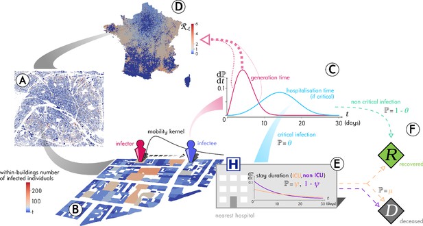
Outline of the Epidemap simulation framework.
(A) The 66 millions inhabitants of metropolitan France are explicitly mapped to housing buildings following cartographic and demographic data. (B) At each time point of the simulation, the number of infected individuals in each building of the country is recorded, as well as the time past since each got infected (the panel shows the Paris area). (C) Every day, individuals can randomly move from their home to other buildings according to a mobility kernel and meet other people. If an infected individual encounters a susceptible host, a transmission event can occur. (D) The contagiousness of a infected individual varies depending on the time since infection. (E) A small fraction of infected individuals develop a critical form of the disease that requires their hospitalisation to the nearest facility. Clinical dynamics can be assumed not to affect transmission dynamics because more than 95% of the secondary transmission events occur before hospital admission.
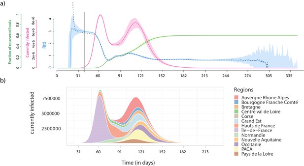
Epidemiological dynamics at the national (a) and regional (b) level.
(a) The daily prevalence (the number of infected individuals) is in red, the temporal reproduction number () in blue, and the cumulative number of recovered individuals in green. Shaded areas show the 95% sample quantiles of 100 stochastic simulations. The dashed line shows the median calculated on the case incidence data. (b) Each colour shows the prevalence in a French region.
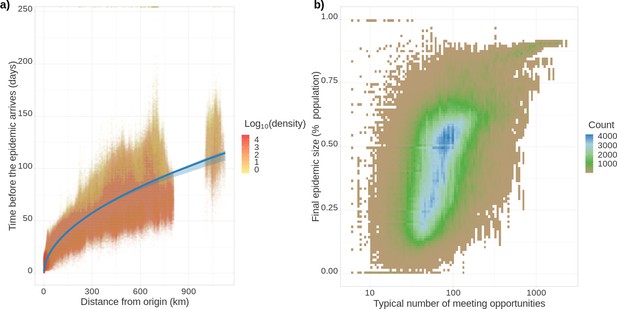
Epidemic arrival date and size at the district level.
(a) Effect of the distance from the epicentre on the number of days until the epidemic begins in a district. The colour indicates the population density in the district (number of inhabitants divided by the district’s surface). (b) District final epidemic size as a function of the characteristic distance between two individuals normalised by the average dispersal distance. The latter is computed as , where is the log-normal distribution of daily individual covered distance. Both panels show the value for 35,234 French districts and 100 stochastic simulations.
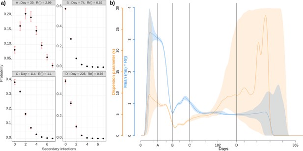
Individual reproduction number dynamics.
(a) Distribution obtained over the whole population on 4 different days post outbreak. (b) Daily variation of the mean (in blue) and dispersion (in orange) of the distribution of individual reproduction numbers, which is assumed to follow a Negative Binomial distribution (Lloyd-Smith et al., 2005). Shaded areas show the 95% CI.
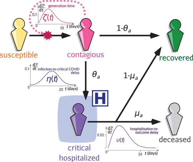
Infection model flow chart.
Susceptible individuals (yellow figurine), are exposed to viral transmission from contagious individuals (pink figurine). Once infected, a host is more or less contagious depending on the time since contamination according to distribution called the generation time (and usually parameterised using the empiric serial interval). A fraction , the value of which depends on the age of the host , will develop a critical infection and be admitted to a hospital (purple figurine) according to the complication delay distribution . The complementary fraction is assumed to recover with perfect and long-lasting immunity (green figurine). This compartment is also reachable after hospitalisation with the age-dependent probability , after the discharge delay distribution . The complementary fraction eventually dies from COVID-19. See Sofonea et al., 2021 for additional details.
Videos
Density of residents in ICU throughout an uncontrolled epidemic.
The top panel shows the value at a fine geographical scale (French ‘canton’) and the bottom panel shows the total density at the national level along with the corresponding temporal reproduction number ().
Density of infected people / 100 k residents for an uncontrolled epidemic.
The top panel shows the value at a fine geographical scale (French ‘canton’) and the bottom panel shows the total density at the national level along with the corresponding temporalreproduction number (R(t)).
Complete transmission chains colored by chain length of an uncontrolled epidemic.
Tables
Lognormal randomly choosen values and INSEE statistic of the distance between residential and distant building.
Original datas (INSEE, 2016) and fitting.
| INSEE statistic | ||
|---|---|---|
| lt10 km | 32.9% | 33.7% |
| 10 km km | 30.6% | 30.5% |
| 20 km km | 15.5% | 16.0% |
| 30 km km | 12.7% | 12.5% |
| 50 km km | 6.8% | 5.8% |
| gt100 km | 1.5% | 1.5% |
Parameters used for the transmission model in the simulations.
LN stands for log-normal, We for Weibull.
| Name | Description | Value | Reference |
|---|---|---|---|
| Number of agents (population size) | 6.6E7 | INSEE, 2019 | |
| Number of buildings visited during the day (+ home) | 3 | Schneider et al., 2013 | |
| Individual dispersal kernel distance | fit of INSEE, 2016 | ||
| N1 | Maximum daily number of agent met (distant) | 17 | user-defined |
| N2 | Maximum daily number of agent met (at home) | 5 | user-defined |
| Contagiousness days after infection | Nishiura et al., 2020 | ||
| Transmission probability per contact | Variant Technical group, 2021 |
Parameters used for the clinical progression of the infections in the simulations.
These parameters do not affect virus spread. LN stands for log-normal, We for Weibull.
| Name | Description | Value | Reference |
|---|---|---|---|
| µ | Hospital mortality rate | 56% | Santé Publique France, 2020 |
| ICU admission daily probability for a severely infected patient | Linton et al., 2020 | ||
| ICU departure daily probability | Linton et al., 2020 | ||
| Probability for a severely infected patient of age to die | Verity et al., 2020 |


