Hippocampal sharp wave-ripples and the associated sequence replay emerge from structured synaptic interactions in a network model of area CA3
- Institute of Experimental Medicine, Eötvös Loránd Research Network, Hungary
- Faculty of Information Technology and Bionics, Pázmány Péter Catholic University, Hungary
- Alfréd Rényi Institute of Mathematics, Eötvös Loránd Research Network, Hungary
- Institute for Computer Science and Control, Eötvös Loránd Research Network, Hungary
Figures
Figure 1 with 2 supplements
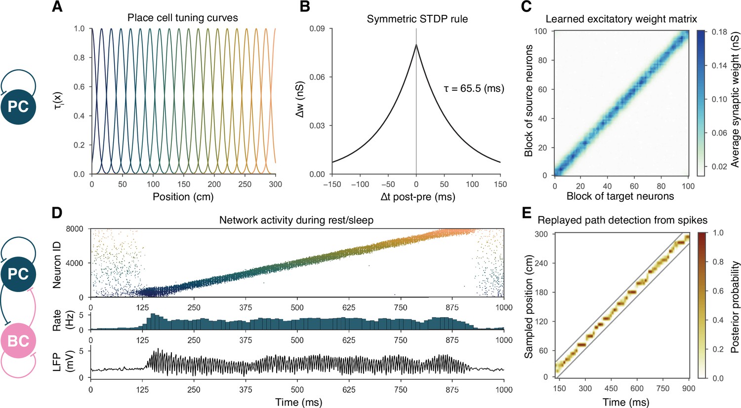
Overview of learning and the spontaneous generation of sharp wave-ripples (SWRs) and sequence replay in the model.
(A) Tuning curves (Equation (1)) of exemplar place cells covering the whole 3-m-long linear track. (B) Broad, symmetric spike-timing-dependent plasticity (STDP) kernel used in the learning phase. The time constant was fit directly to experimental data from Mishra et al., 2016. (C) Learned excitatory recurrent weight matrix. Place cells are ordered according to the location of their place fields; neurons with no place field in the environment are scattered randomly among the place cells. Actual dimensions are 8000 * 8000, but, for better visualization, each pixel shown represents the average of an 80 * 80 square. (D) Pyramidal cell (PC) raster plot is shown in the top panel, color-coded, and ordered as the place fields in (A). PC population rate (middle), and local field potential (LFP) estimate (bottom panel), corresponding to the same time period. (E) Posterior matrix of the decoded positions from spikes within the high activity period shown in (D). Gray lines indicate the edges of the decoded, constant velocity path.
Figure 1—figure supplement 1
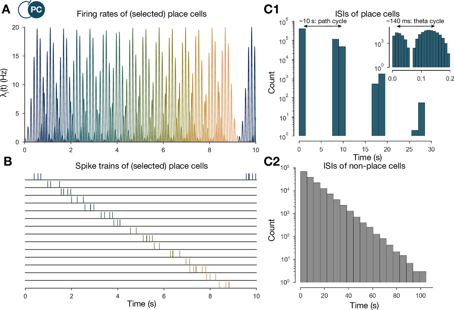
The generation of the spike trains of pyramidal cells (PCs) in the exploration phase.
(A) Firing rates of exemplar place cells covering the whole 3-m-long linear track. In contrast to the spatial tuning curves shown in Figure 1A (Equation (1)), these are time-dependent rates modulated by theta oscillation and phase precession (Equation (2)). (B) Exemplar spike trains generated based on the firing rates shown in (A). (Spike trains used in the learning phase were 400 s long. For the purpose of visualization, only the beginning is shown here.) (C) Interspike interval (ISI) distribution of the generated spike trains. ISIs of place cells (C1) (inset is a zoom into the same distribution at a finer timescale to show theta modulation) and nonplace cells (C2).
Figure 1—figure supplement 2
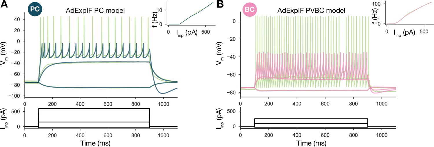
Single-cell models.
(A) Fitted AdExpIF pyramidal cell (PC) model (blue) and experimental traces (green) are shown in the top panel. The amplitudes of the 800-ms-long step current injections shown at the bottom were as follows: –0.04, 0.15, and 0.6 nA. (B) Fitted ExpIF parvalbumin-containing basket cell (PVBC) model (pink) and experimental traces (green) are shown in the top panel. The amplitudes of the 800-ms-long step current injections shown at the bottom were as follows: –0.03, 0.09, and 0.25 nA. Insets show the f–I curve of the in vitro (green) and in silico (red) cells. For parameters of the cell models, see Table 2.
Figure 2 with 2 supplements
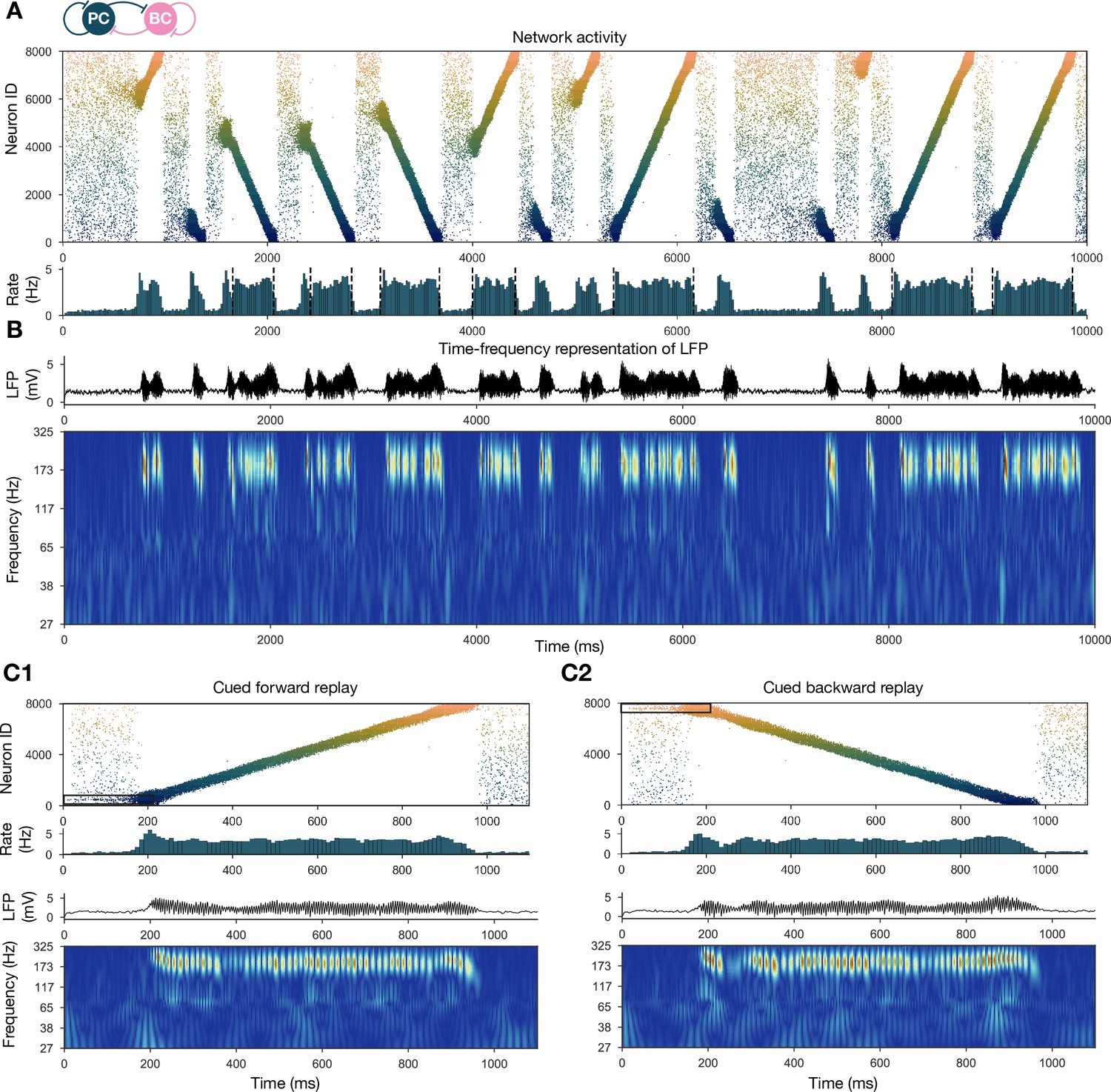
Forward and backward replay events, accompanied by ripple oscillations, can occur spontaneously but can also be cued.
(A) Pyramidal cell (PC) raster plot of a 10-s-long simulation, with sequence replays initiating at random time points and positions and propagating either in forward or backward direction on the top panel. PC population firing rate is plotted below. Dashed vertical black lines indicate the periods marked as sustained high-activity states (above 2 Hz for at least 260 ms), which are submitted to automated spectral and replay analysis. (B) Estimated local field potential (LFP) in the top panel and its time-frequency representation (wavelet analysis) below. (C) Forward and backward sequence replays resulting from targeted stimulation (using 200-ms-long 20 Hz Poisson spike trains) of selected 100-neuron subgroups, indicated by the black rectangles in the raster plots. (C1) Example of cued forward replay. PC raster plot is shown at the top with PC population rate, LFP estimate, and its time-frequency representation (wavelet analysis) below. (C2) Same as (C1), but different neurons are stimulated at the beginning, leading to backward replay.
Figure 2—figure supplement 1

The step-size distribution of the decoded paths is much wider than expected.
(A) Posterior matrix of the decoded positions from spikes within a selected high-activity state (first one from Figure 2A). Thick gray lines indicate the edges of the decoded, constant velocity path. Thin gray line shows the decoded path by connecting the weighted average positions in every 10-ms-long time step. (B) Step sizes from the decoded, variable velocity path (see A) for the same period (first high-activity state in Figure 2A). The horizontal dashed black line shows the average or predicted step size within the given period. (C1) Skewed distribution of observed step sizes (in gray) and the predicted (from evenly spacing) step-size distribution (in red) for more than a hundred replay events (similar to the one in A and B). Inset shows the same distributions at smaller scales. (C2) Cumulative distribution of the observed and predicted step sizes shown in (C1). Observed vs. predicted distributions differ significantly (two-sample Kolmogorov–Smirnov test).
Figure 2—figure supplement 2
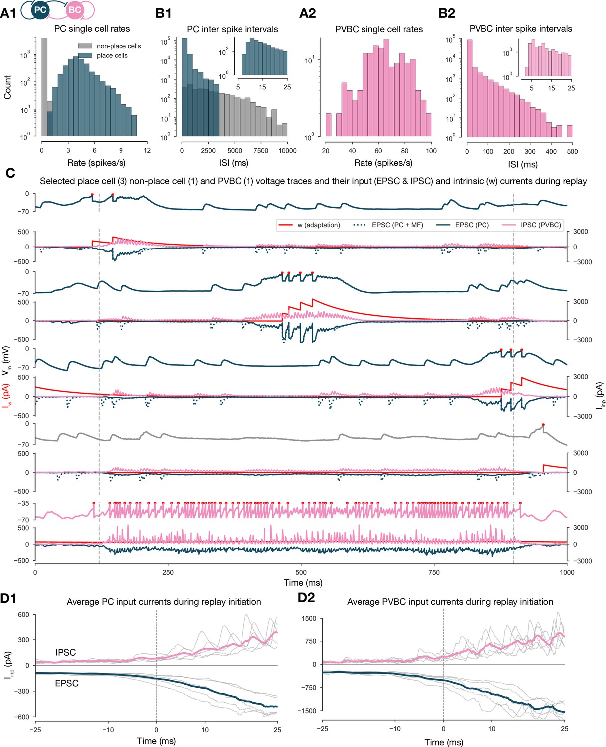
Single-cell characteristics during network simulations.
(A) Distributions of single pyramidal cell (PC) (A1) and parvalbumin-containing basket cell (PVBC) (A2) firing rates during the 10-s-long simulation shown in Figure 2. (B) Distributions of interspike intervals (ISIs) of PCs (B1) and PVBCs (B2) in the 10-s-long simulation shown in Figure 2. (C) Voltage traces of selected place cells from the beginning, middle, and end of the track, a nonplace cell and a PVBC on top, and their input currents (EPSC (excitatory postsynaptic current) in blue, IPSC (inhibitory postsynaptic current) in pink, y-axis on the right) and intrinsic adaptation current w (red, y-axis on the left) at the bottom of each panel, during a full forward replay. Dashed vertical lines indicate the period marked as high-activity state. (D) Synaptic input currents of PCs (D1) and PVBCs (D2) during sequence replay initiation. Gray lines are the averages of the EPSCs and IPSCs of 400 PCs and 30 PVBCs, respectively (similar to the ones shown in C). Individual gray lines correspond to individual high-activity states (n = 7, see Figure 2A). Dashed vertical lines (at 0 ms) indicate the beginning of the periods marked as high-activity states (see Figure 2A). Colored lines represent the grand average EPSC (blue) and IPSC (pink) arriving at PCs (D1) and PVBCs (D2) during sharp wave-ripple (SWR) initiation.
Figure 3 with 1 supplement
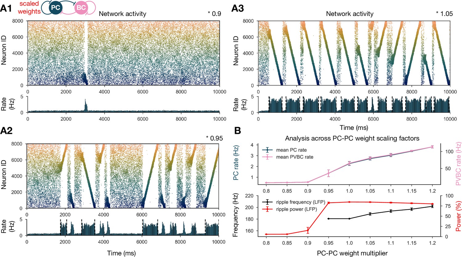
Sharp waves, ripple oscillations, and replay are robust with respect to scaling the recurrent excitatory weights.
(A) Pyramidal cell (PC) raster plots on top and PC population rates at the bottom for E-E scaling factors 0.9 (A1), 0.95 (A2), and 1.05 (A3). (Scaling factor of 1.0 is equivalent to Figure 2A.) Dashed vertical black lines have the same meaning as in Figure 2A. (B) Analysis of selected indicators of network dynamics across different E-E weight scaling factors (0.8–1.2). Mean PC (blue) and parvalbumin-containing basket cell (PVBC) (pink) population rates are shown on top. The frequency of significant ripple oscillations (black) and the percentage of power in the ripple frequency range (red) in the estimated local field potential (LFP) is shown at the bottom. Errors bars indicate standard deviation and are derived from simulations with five different random seeds. See also Figure 3—figure supplement 1.
Figure 3—figure supplement 1
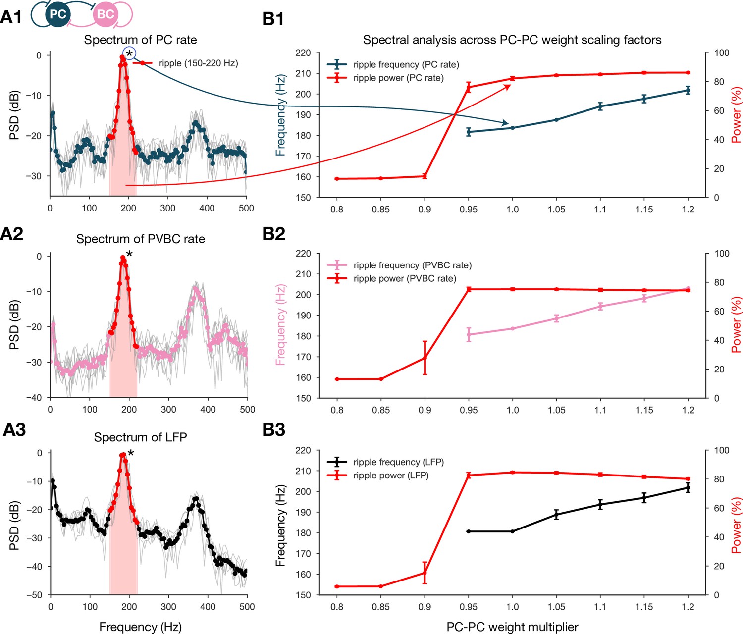
Spectral analysis of network dynamics across different pyramidal cell-pyramidal cell (PC-PC) weight scaling factors.
(A) Power spectral densities (PSDs) of PC (A1) and parvalbumin-containing basket cell (PVBC) (A2) population rates and estimated local field potential (LFP) (A3). Gray lines correspond to individual high-activity states (n = 14) shown in Figure 2A, while the thicker-colored lines are their averages. Ripple frequency range (150–220 Hz) is highlighted in red. Shaded red area below the curves indicates the power in the ripple range. (B) Spectral analysis of network dynamics across different E-E weight scaling factors (0.8–1.2). The frequency of any significant ripple oscillation (black) and the percentage of power in the ripple band (red) are shown for PC (B1) and PVBC (B2) population rates and estimated LFP (B3). (B3) is the same as the bottom panel of Figure 3B, and it is duplicated here only to show how similar the curves are for the rates and the estimated LFP.
Figure 4
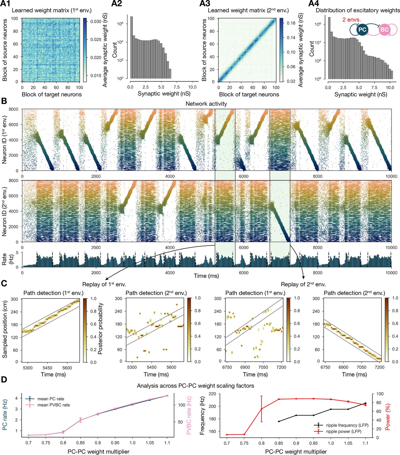
Two distinct environments can be learned and replayed by the network.
(A) Learned excitatory recurrent weight matrices. (A1) Weights after learning the first environment. Note that the matrix appears random because neurons are arranged according to their place field location in the second environment, which has not been explored at this point. (A3) Weights after learning in the second environment. (A2, A4) Distribution of nonzero synaptic weights in the learned weight matrices in (A1) and (A2), respectively. (B) Pyramidal cell (PC) raster plots: in the top panel, neurons are ordered and colored according to the first environment; in the middle panel, neurons are ordered and colored according to the second environment; and PC population rate is shown at the bottom (see Figure 2A) from a simulation run with 0.9* the modified weight matrix shown in (A3). (C) Posterior matrices of decoded positions from spikes (see Figure 1E) within two selected high-activity periods (8th and 10th from B). From left to right: decoding of replay in first environment (eighth event from B) according to the first (significant) and second environment; decoding of replay in second environment (10th event from B) according to the first and second (significant) environment. (D) Analysis of selected network dynamics indicators across different E-E weight scaling factors (0.7–1.1) as in Figure 3B.
Figure 5

Learning with an asymmetric spike-timing-dependent plasticity (STDP) rule leads to the absence of backward replay.
(A) Asymmetric STDP kernel used in the learning phase. (B) Learned excitatory recurrent weight matrix. (C) Distribution of nonzero synaptic weights in the weight matrix shown in (B). (D) Pyramidal cell (PC) raster plot on top and PC population rate at the bottom (see Figure 2A) from a simulation run with the weight matrix shown in (B). (E) Posterior matrix of the decoded positions from spikes (see Figure 1E) within a selected high-activity state (sixth one from D). (F) Analysis of selected network dynamics indicators across different E-E weight scaling factors (0.8–1.2) as in Figure 3B.
Figure 6

Altering the structure of recurrent excitatory interactions changes the network dynamics but altering the weight statistics has little effect.
(A1) Binarized (largest 3% and remaining 97% nonzero weights averaged separately) recurrent excitatory weight matrix. (Derived from the baseline one shown in Figure 1C.) (A2) Distribution of nonzero synaptic weights in the learned weight matrix shown in (A1). (B) Pyramidal cell (PC) raster plot on top and PC population rate at the bottom (see Figure 2A) from a simulation run with 1.1* the binarized weight matrix shown in (A). (C) Analysis of selected network dynamics indicators across different E-E weight scaling factors (0.9–1.3) as in Figure 3B. (D1) Column-shuffled recurrent excitatory weight matrix. (Derived from the baseline one shown in Figure 1C.) (D2) Distribution of nonzero synaptic weights in the weight matrix shown in (D1) (identical to the distribution of the baseline weight matrix shown in Figure 1C). (E) PC raster plot on top and PC population rate at the bottom from a simulation run with the shuffled weight matrix shown in (D1). (F) Analysis of selected network dynamics indicators across different E-E weight scaling factors (1.0–4.0) as in Figure 3B. Note the significantly extended horizontal scale compared to other cases.
Figure 7
Sequential replay requires firing rate adaptation in the pyramidal cell (PC) population.
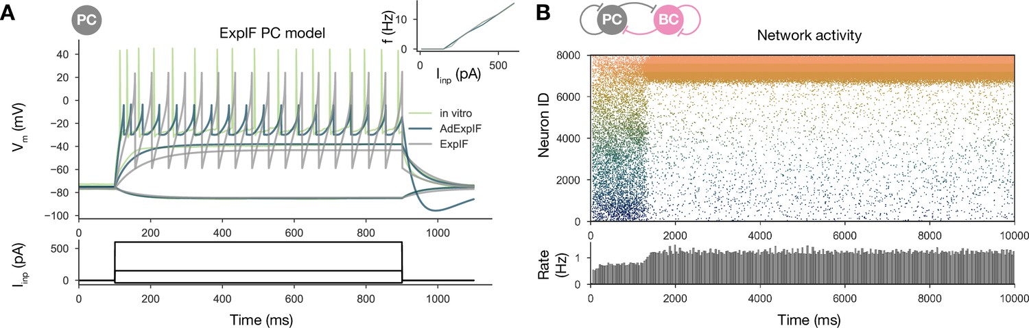
(A) Voltage traces of fitted AdExpIF (blue) and ExpIF (gray) PC models and experimental traces (green) are shown in the top panel. Insets show the f–I curves of the in vitro and in silico cells. The amplitudes of the 800-ms-long step current injections shown at the bottom were as follows: –0.04, 0.15, and 0.6 nA. For parameters of the cell models, see Table 2. (B) PC raster plot of a 10-s-long simulation with the ExpIF PC models, showing stationary activity in the top panel. PC population rate is shown below.
Figure 8
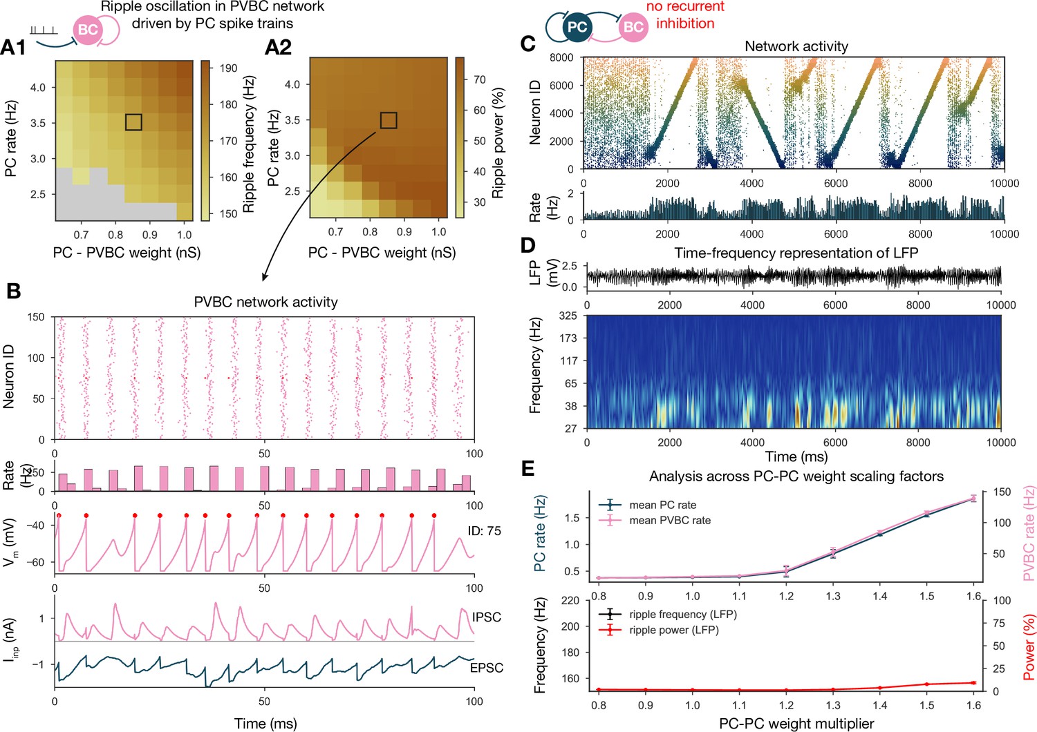
Generation of ripple oscillations relies on recurrent connections within the parvalbumin-containing basket cell (PVBC) population.
(A) Significant ripple frequency (A1) and ripple power (A2) of a purely PVBC network, driven by (independent) spike trains mimicking pyramidal cell (PC) population activity. Gray color in (A1) means no significant ripple peak. (B) From top to bottom: raster plot, mean PVBC rate, voltage trace (of a selected cell), EPSCs, and IPSCs of the selected cell from the middle (100-ms-long window) of a simulation used for (A). Ripple frequency and power corresponding to this simulation are marked with a black rectangle in (A1) and (A2). (C) PC raster plot on top and PC population rate at the bottom from a simulation run with a network with 1.3* baseline E-E weight matrix but without any PVBC-PVBC synapses, featuring stochastic forward and backward replays but no ripple oscillation (see below). (D) Estimated local field potential (LFP) in the top panel and its time-frequency representation (wavelet analysis) below. (Compared to Figure 2B, there is increased power in the gamma range, but no ripple frequency oscillation.) (E) Analysis of selected network dynamics indicators across different E-E weight scaling factors (0.8–1.6) as in Figure 3B.
Tables
Table 1
List of modeling assumptions.
| 1 | In the absence of unified datasets, it was assumed that published parameters from different animals (mouse/rat, strain, sex, age) can be used together to build a general model. |
| 2 | Connection probabilities were assumed to depend only on the presynaptic cell type and to be independent of distance. |
| 3 | Each pyramidal cell was assumed to have a place field in any given environment with a probability of 50%. For simplicity, multiple place fields were not allowed. |
| 4 | When constructing the ‘teaching spike trains’ during simulated exploration, place fields were assumed to have a uniform size, tuning curve shape, and maximum firing rate. |
| 5 | For simplicity, all synaptic interactions in the network were modeled as deterministic conductance changes. Short-term plasticity was not included, and long-term plasticity was assumed to operate only in the learning phase. |
| 6 | When considering the nonspecific drive to the network in the offline state, it was assumed that the external input can be modeled as uncorrelated random spike trains (one per cell) activating strong synapses (representing the mossy fibers) in the pyramidal cell population. |
| 7 | Some fundamental assumptions are inherited from common practices in computational neuroscience; these include modeling spike trains as Poisson processes, capturing weight changes with additive spike-timing-dependent plasticity, describing cells with single-compartmental AdExpIF models, modeling a neuronal population with replicas of a single model, and representing synapses with conductance-based models with biexponential kinetics. |
| 8 | When comparing our model to in vivo data, an implicit assumption was that the behavior of a simplified model based on slice constraints can generalize to the observed behavior of the full CA3 region in vivo, in the context of studying the link between activity-dependent plasticity and network dynamics. |
Table 2
Optimized parameters of pyramidal cell (PC) (AdExpIF and ExpIF) and parvalbumin-containing basket cell (PVBC) models.
Physical dimensions are as follows: : pF; and : nS; , , , , and : mV; and : ms; : pA.
| PC | 180.13 | 4.31 | –75.19 | 4.23 | –24.42 | –3.25 | –29.74 | 5.96 | 84.93 | –0.27 | 206.84 |
| PC | 344.18 | 4.88 | –75.19 | 10.78 | –28.77 | 25.13 | –58.82 | 1.07 | - | - | - |
| PVBC | 118.52 | 7.51 | –74.74 | 4.58 | –57.71 | –34.78 | –64.99 | 1.15 | 178.58 | 3.05 | 0.91 |
Table 3
Synaptic parameters (taken from the literature or optimized).
Physical dimensions are as follows: : nS; , , and td (synaptic delay): ms; and connection probability is dimensionless. GC stands for the granule cells of the dentate gyrus. ( synapses are referred as mossy fibers.) Sym. and asym. indicate maximal conductance parameters obtained for networks trained with the symmetric and the asymmetric spike-timing-dependent plasticity (STDP) kernel, respectively. PC: pyramidal cell; PVBC: parvalbumin-containing basket cell.
| td | ||||||
|---|---|---|---|---|---|---|
| Sym. | Asym. | |||||
| PC PC | 0.1–6.3 | 0–15 | 1.3 | 9.5 | 2.2 | 0.1 |
| PC PVBC | 0.85 | 1 | 4.1 | 0.9 | 0.1 | |
| PVBC PC | 0.65 | 0.3 | 3.3 | 1.1 | 0.25 | |
| PVBC PVBC | 5 | 0.25 | 1.2 | 0.6 | 0.25 | |
| GC PC | 19.15 | 21.5 | 0.65 | 5.4 | - | - |
Additional files
Download links
A two-part list of links to download the article, or parts of the article, in various formats.
Downloads (link to download the article as PDF)
Open citations (links to open the citations from this article in various online reference manager services)
Cite this article (links to download the citations from this article in formats compatible with various reference manager tools)
Hippocampal sharp wave-ripples and the associated sequence replay emerge from structured synaptic interactions in a network model of area CA3
eLife 11:e71850.
https://doi.org/10.7554/eLife.71850


