In situ X-ray-assisted electron microscopy staining for large biological samples
- Princeton Neuroscience Institute, Princeton University, United States
- Paul Scherrer Institute, Switzerland
Figures
Figure 1 with 3 supplements
X-ray assisted staining.
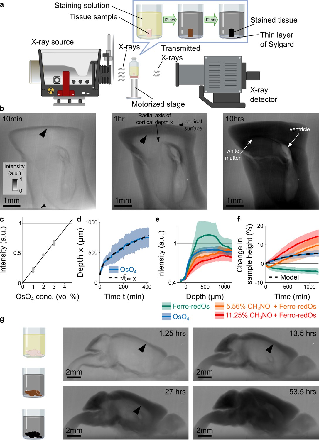
(a) Experimental setup. The sample was glued into a thin layer of Sylgard and sits in staining solution in a sealed glass vial on a motorized stage. X-rays are emitted from an X-ray source, pass through the sample, and the spatial distribution of the transmitted X-rays is detected and used to form a projection image of the X-ray absorption in the sample. Over time, the heavy metals diffuse into the tissue and the accumulation of heavy metals change the X-ray absorption properties of the sample. For the quantitative results presented in this study we used cylindrical tissue samples extracted with a 4 mm diameter biopsy punch from the cortex of mice. (b) Projection images of a 4 mm punch of mouse cortex incubated in 2% buffered osmium tetroxide (OsO4) solution after 10 min, 1 hr, and 10 hr. The osmium diffuses passively from the cortical surface and the brain ventricles into the tissue and forms a staining front of tissue-bound osmium (large arrowhead) that moves towards the center of the sample as time progresses. The accumulation of heavy metals results in an increase in the pixel intensity (a.u.) of the X-ray projection image, which was measured along the radial axis of cortical depth from the cortical surface towards the white matter. The small arrowhead indicates the upper edge of the 2 mm thin layer of Sylgard. (c) Measured pixel intensities of the X-ray projection images for different concentrations of buffered OsO4 solutions. The higher/darker the intensity, the more X-rays are absorbed. The pixel intensity/X-ray absorption scales linearly with the concentration/density of osmium (black line, Pearson correlation coefficient r=0.99, <10–6; n=3 for each concentration). (d) Propagation of the staining front in 4 mm brain punches immersed in 2% buffered OsO4 solution (n=13) measured along the radial axis of cortical depth (mean ±s.d.). The propagation can be fitted by a quadratic model (dashed black lines) in which the penetration depth x of the staining front is proportional to the square root of the incubation time t (residual standard error: SEres = 14.68 μm). (e) Intensity profiles of the spatial heavy metal accumulation after t=20 hr of incubation in 2% buffered OsO4 (blue, n=13), Ferro-redOs (green, n=6). Ferro-redOs with 5.56% (orange, n=4) and 11.25% formamide (red, n=4) solutions (mean ±s.d.). In Ferro-redOs the heavy metal staining is not homogenous and there is a more densely stained tissue band at a depth of 300–800 μm. (f) Tissue expansion quantified as change in sample height of aldehyde-fixed brain punches immersed in OsO4 (blue, n=13), Ferro-redOs (green, n=6), Ferro-redOs with 5.56% (orange, n=4) and 11.25% formamide (red, n=4), respectively, as a function of the immersion duration (mean ±s.d.). All solutions were buffered by cacodylate. A monomolecular growth model was fitted to the average tissue expansion in OsO4 solution (black dashed line, residual standard error SEres = 0.06%). (g) In situ X-ray-assisted staining of large tissue samples. The images show projections of a whole mouse brain incubated in 2% buffered OsO4 at different points in time across 2.5 days. The arrowheads indicate the location of the staining front of accumulated osmium. Scale bar 2 mm.
-
Figure 1—source data 1
Experimentally measured accumulation of heavy metals (blue traces) in buffered 2% OsO4 solution in n=13 different samples.
The corresponding simulated model was fitted individually to the experimental data of each sample (black traces). The first row of every sample shows the temporal profile of osmium accumulation at different cortical depths, while the second row shows the spatial profile of osmium accumulation at different times after staining onset. The black circles indicate the location of axon tracts that tended to accumulate osmium faster and stronger. The third row shows the measured spatial-temporal accumulation of osmium (left), the corresponding fitted model simulations (middle) and the distribution of osmium in projection images of the sample at the beginning of the experiment and after about 22 hr of incubation (right).
- https://cdn.elifesciences.org/articles/72147/elife-72147-fig1-data1-v2.pdf
-
Figure 1—source data 2
Experimentally measured accumulation of heavy metals in a buffered solution of 2% OsO4 reduced with 2.5% potassium ferrocyanide K4[Fe(CN)6] (Ferro-redOs) in n=6 different samples.
The first row shows the temporal profile of osmium accumulation at different cortical depths, while the second row shows the spatial profile of osmium accumulation at different times after staining onset. The black circles indicate the location of axon tracts that tended to accumulate osmium faster and stronger. The third row shows the measured spatial-temporal accumulation of osmium (left) and the corresponding distribution of osmium in projection images of the sample at the beginning of the experiment and after about 22 hoursr of incubation (right).
- https://cdn.elifesciences.org/articles/72147/elife-72147-fig1-data2-v2.pdf
-
Figure 1—source data 3
Experimentally measured accumulation of heavy metals in buffered 2% Ferro-redOs solution with 5.56% formamide in n=4 different samples.
The first row of every sample shows the temporal profile of osmium accumulation at different cortical depths, while the second row shows the spatial profile of osmium accumulation at different times after staining onset. The black circles indicate the location of axon tracts that tended to accumulate osmium faster and stronger. The third row shows the measured spatial-temporal accumulation of osmium (left) and the corresponding distribution of osmium in projection images of the sample at the beginning of the experiment and after about 22 hoursr of incubation (right).
- https://cdn.elifesciences.org/articles/72147/elife-72147-fig1-data3-v2.pdf
-
Figure 1—source data 4
Experimentally measured accumulation of heavy metals in buffered 2% Ferro-redOs solution with 11.25% formamide in n=4 different samples.
The first row of every sample shows the temporal profile of osmium accumulation at different cortical depths, while the second row shows the spatial profile of osmium accumulation at different times after staining onset. The black circles indicate the location of axon tracts that tended to accumulate osmium faster and stronger. The third row shows the measured spatial-temporal accumulation of osmium (left) and the corresponding distribution of osmium in projection images of the sample at the beginning of the experiment and after about 22 hoursr of incubation (right).
- https://cdn.elifesciences.org/articles/72147/elife-72147-fig1-data4-v2.pdf
-
Figure 1—source data 5
Experimentally measured accumulation of heavy metals in a buffered solution of 2% OsO4 reduced with 2.5% potassium ferricyanide K3[Fe(CN)6] (Ferri-redOs) in n=2 different samples.
The first row shows the temporal profile of osmium accumulation at different cortical depths, while the second row shows the spatial profile of osmium accumulation at different times after staining onset. The black circles indicate the location of axon tracts that tended to accumulate osmium faster and stronger. The third row shows the measured spatial-temporal accumulation of osmium (left) and the corresponding distribution of osmium in projection images of the sample at the beginning of the experiment and after about 22 hoursr of incubation (right).
- https://cdn.elifesciences.org/articles/72147/elife-72147-fig1-data5-v2.pdf
Figure 1—figure supplement 1
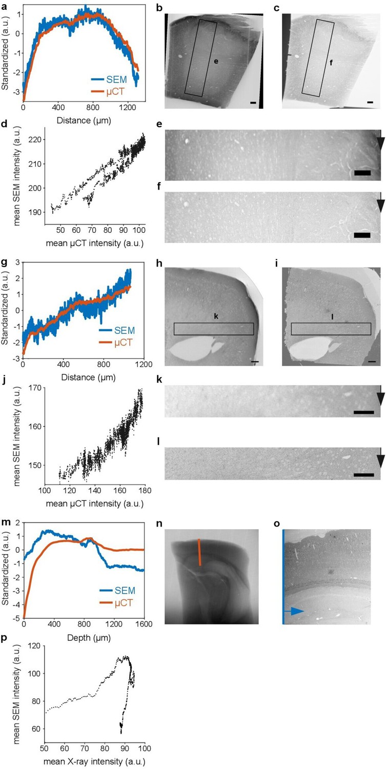
As reported previously (Mikula and Denk, 2015, Figure 4b), X-ray imaging exhibits a contrast similar to scanning electron microscopy (SEM).
In the following μCT reslices and X-ray projection images of en bloc stained brain tissue are compared to the corresponding serial-section SEM image from the same tissue block. (a-g) Covariation of the standardized μCT and standardized SEM intensity in the same tissue area. The μCT and SEM pixel intensities were averaged along the vertical direction (black arrow) in the regions of interest (ROI) shown in e+f/k+l. (b-h) μCT reslice and (c-i) SEM overview image of the same tissue section. The black rectangle indicates the location of the ROI shown in e+f/k+l. (d-j) Scatter plot of the average SEM pixel intensity versus the average μCT reslice pixel intensity in the ROI shown in e+f/k+l, averaged along the vertical direction (black arrow) (d: r=0.923, p<1e-9, j: 0.944, p<1e-9; Pearson correlation coefficient). (m) Covariation of the standardized X-ray and standardized SEM intensity as a function of cortical depth. The X-ray intensity was measured along the red line in the X-ray projection image shown in (n). The SEM intensity was measured along the blue line in the SEM image shown in (o) after averaging the intensity values along the horizontal axis (indicated by the blue arrow). The intensities were standardized by subtracting the mean and dividing by the standard deviation. Note, the X-ray intensity corresponds to a projection through the entire 4 mm brain punch, whereas the SEM intensity has been only accumulated over the width of about 1.5 mm of the original punch in b, because the embedded block was trimmed to a width of about 1.5 mm for ultra-thin section collection. (n) X-ray projection image of a 4 mm punch of brain tissue that was incubated in 2% buffered OsO4 for 20 hours. (o) Low-resolution SEM image of a 40 nm thick section (same as in Figure 1—figure supplement 3) from the sample in n, after dehydration with ethanol and acetonitrile and embedding in hard Epon. The section was collected orthogonally to the transverse plane of the punch at a depth of about 1 mm from the sample surface. The image has been rescaled to account for the shrinkage of the sample during the dehydration and embedding as well as for compression from sectioning. (p) Scatter plot of the average SEM pixel intensity versus the X-ray projection image pixel intensity (r=0.243, p<4.45e-9; Pearson correlation coefficient). Scale bar 100 μm.
Figure 1—figure supplement 2
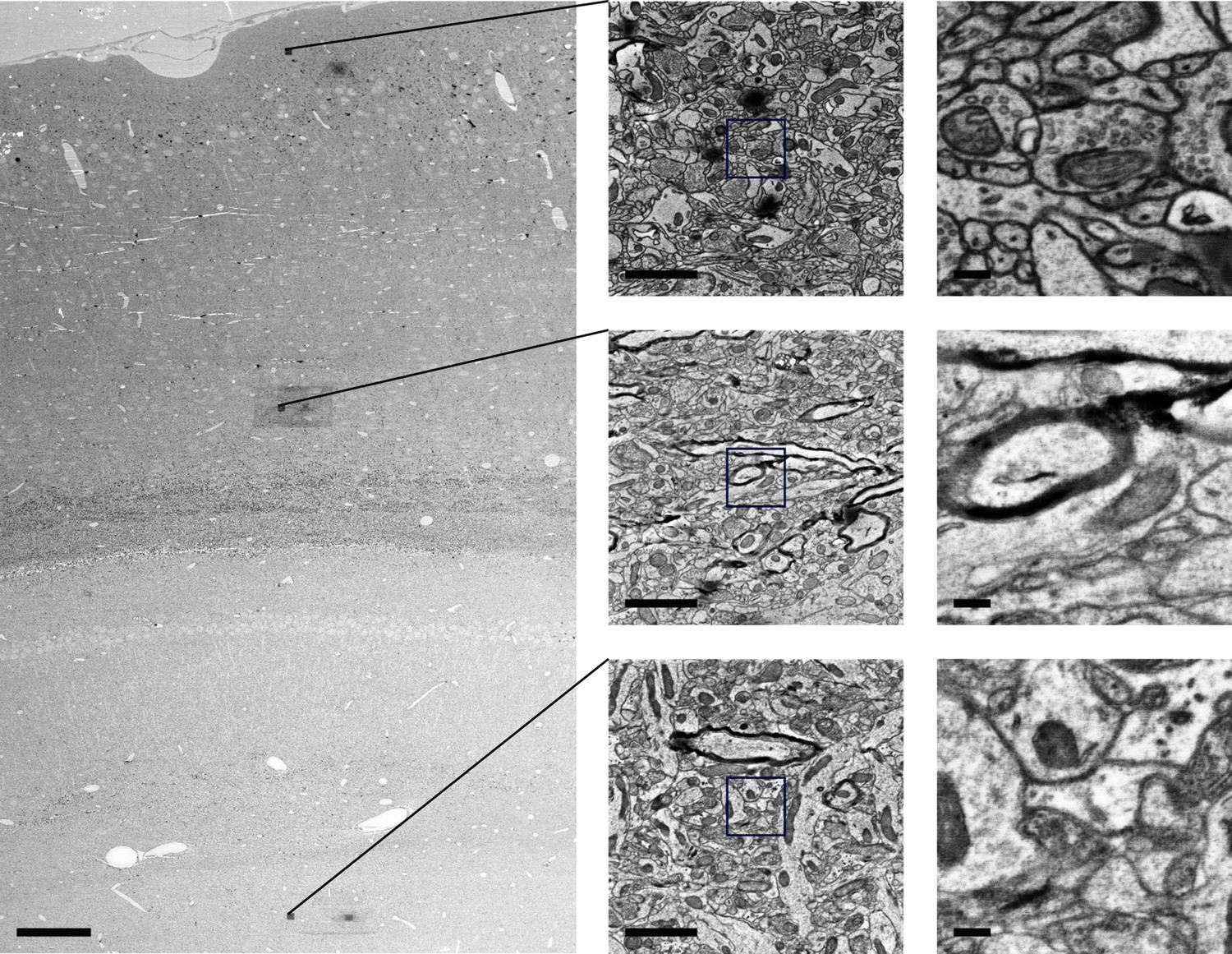
Ultrastructural preservation at various tissue depths after 20 hr of X-ray-assisted staining with 2% buffered OsO4.
First, a 4 mm punch of aldehyde-fixed brain tissue was immersed in 2% buffered OsO4 monitored using X-ray assisted staining for 20 hr. Afterwards, the sample was washed, dehydrated with ethanol and acetonitrile and embedded in hard Epon. Next, 40-nm-thick sections of the trimmed sample block were collected orthogonally to the transverse plane of the brain punch at a depth of about 1 mm from the tissue surface. Electron microscopy images of the section were acquired at low magnification (left) as well as high magnification at different cortical depths (middle +right column) using scanning electron microscopy. Scale bars: Left: 100 μm, middle column: 2 μm, right column: 200 nm.
Figure 1—figure supplement 3
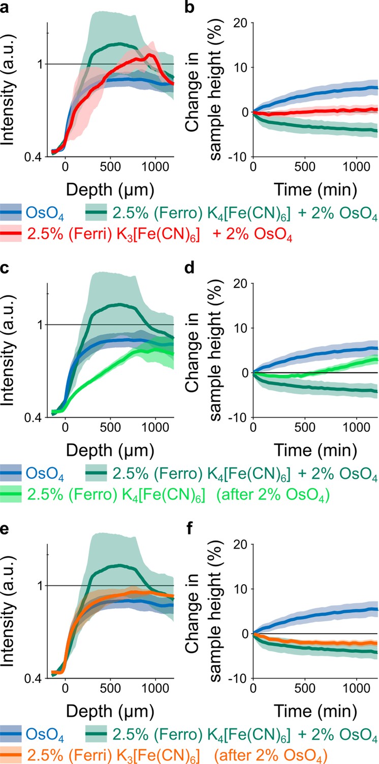
Spatial intensity profiles of accumulated heavy metals after t=20 hr of incubation (left column) and temporal tissue expansion profiles (right column) for different osmium reduction protocols in comparison to 2% buffered OsO4 (blue, n=13) and buffered solution of 2% OsO4 reduced with 2.5% potassium ferricyanide K4[Fe(CN)6] (green, n=6) (mean ±s.d.).
All solutions were buffered by cacodylate. (a-b) Buffered solution of 2% OsO4 reduced with 2.5% potassium ferricyanide K3[Fe(CN)6] (red, n=2). (c-d) Buffered solution of 2.5% potassium ferrocyanide K4[Fe(CN)6] after 20 hr of incubation in buffered 2% OsO4 solution (light green, n=6). (e-f) Buffered solution of 2.5% potassium ferricyanide K3[Fe(CN)6] after 20 hr of incubation in buffered 2% OsO4 solution (orange, n=4). Note, the intensity for K3[Fe(CN)6] in (e) appears to be about 8% higher than for OsO4 alone. But as can be seen in (f), the tissue height shrinks by about 2% within the 20 hr of incubation. Under the assumption that the shrinkage is isotropic in all three dimensions, this corresponds to a volume reduction of about 5.9% which can explain the observed increase in the intensity.
Figure 2 with 5 supplements
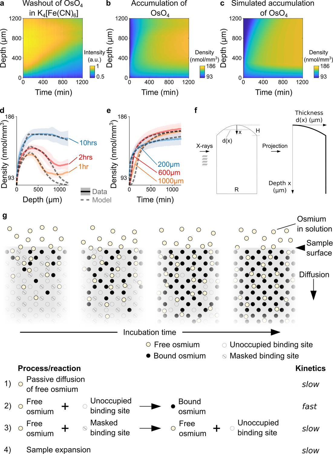
Kinetics and tissue mechanics of electron microscopy staining.
(a) Spatio-temporal washout of osmium in samples incubated in 2.5% potassium ferrocyanide K4[Fe(CN)6] (n=6). The samples have been stained with 2% OsO4 for 22 hrs prior to placing them in K4[Fe(CN)6]. The osmium gets washed out from the sample surface towards the center as the incubation time increases. (b) Average experimentally measured spatio-temporal osmium density (nmol/mm3) accumulation in samples (n=13) immersed in 2% buffered OsO4 solution. Because of the surface curvature of the cortical samples, the tissue thickness decreases towards the surface (x=0) and results in a lower intensity in the projection images (see tissue geometry model in f). (c) Simulated spatio-temporal osmium density (nmol/mm3) accumulation fitted to the average experimental data in b. (d) Density profiles (nmol/mm3) of the spatial accumulation of osmium (n=13, mean ±s.d.) after 1 hr (orange), 2 hrs (red), and 10 hr (blue) of incubation in 2% buffered OsO4 overlaid with the simulation of the diffusion-reaction-advection model (dashed lines). (e) Density profiles (nmol/mm3) of the temporal accumulation of osmium (n=13, mean ±s.d.) at a depth of 200 μm (blue), 600 μm (red), and 1000 μm (orange) during incubation in 2% buffered OsO4, overlaid with the simulation of the diffusion-reaction-advection model (dashed lines). (f) The geometry of the 4 mm brain punches was modeled as a cylinder with a curved surface. The curvature of the sample surface is approximated by a circle with radius , where is diameter of the cylinder and is the height of the curved surface. The projected tissue thickness as a function of the depth x from the sample surface is then given by : , for and , for (g) Diffusion-reaction-advection model for osmium staining. The model combines four coupled processes: (1) Free OsO4 diffuses passively into the tissue and (2) binds to the available binding sites. (3) In the presence of freely diffusing OsO4 previously masked binding sites are slowly turned into additional binding sites for OsO4. (4) The sample expands by about 5% in sample height within 20 hr of incubation (see Figure 1f).
-
Figure 2—source data 1
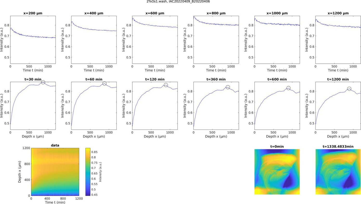
Experimentally measured washout of heavy metals in buffered 2.5% potassium ferrocyanide K4[Fe(CN)6] solution in n=6 different samples that have previously been stained with buffered OsO4 for 22 hr.
The first row of every sample shows the temporal profile of osmium washout at different cortical depths, while the second row shows the spatial profile of osmium washout at different times after staining onset. The black circles indicate the location of axon tracts. The third row shows the measured spatial-temporal washout of osmium (left) and the corresponding distribution of osmium in projection images of the sample at the beginning of the experiment and after about 22 hr of incubation (right).
- https://cdn.elifesciences.org/articles/72147/elife-72147-fig2-data1-v2.pdf
-
Figure 2—source data 2
Experimentally measured washout of heavy metals in buffered 2.5% potassium ferricyanide K3[Fe(CN)6] solution in n=4 different samples that have previously been stained with buffered OsO4 for 22 hrs.
The first row of every sample shows the temporal profile of osmium washout at different cortical depths, while the second row shows the spatial profile of osmium washout at different times after staining onset. The black circles indicate the location of axon tracts. The third row shows the measured spatial-temporal washout of osmium (left) and the corresponding distribution of osmium in projection images of the sample at the beginning of the experiment and after about 22 hoursr of incubation (right).
- https://cdn.elifesciences.org/articles/72147/elife-72147-fig2-data2-v2.pdf
Figure 2—figure supplement 1
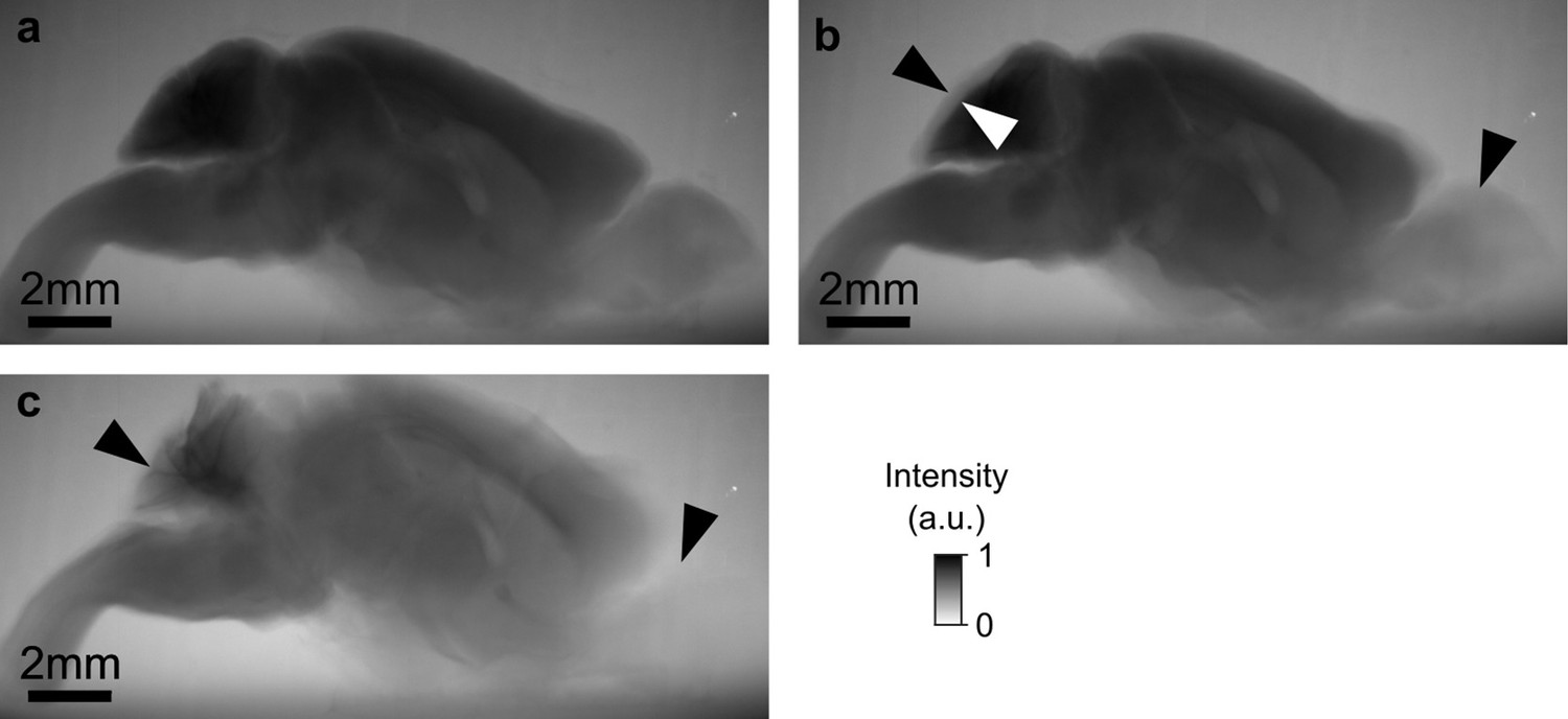
Long incubation in potassium ferrocyanide dissolves and disintegrates the tissue.
(a) Whole mouse brain from Figure 1d after long incubation in osmium. (b) Subsequently, the osmium solution was replaced by 2.5% buffered potassium ferrocyanide solution and the sample was incubated for 16 hr. The tissue clearing is particularly well visible in the cerebellum and olfactory bulbs (arrowheads). (c) After another 108 hr in buffered potassium ferrocyanide a large fraction of the cerebellum and the olfactory bulbs has been dissolved. Scale bar 2 mm.
Figure 2—figure supplement 2
Experimentally measured change in heavy metal accumulation of a sample immersed in double distilled H2O (ddH2O).
Prior to washing the sample with ddH2O the sample has been stained in 2% buffered OsO4 for 22 hr. The first row shows the temporal profile of the change in heavy metal accumulation at different cortical depths, while the second row shows the spatial profile of the change in heavy metal density at different times after washing onset. The black circles indicate the location of axon tracts. The third row shows the measured spatial-temporal change of heavy metal accumulation (left) and the corresponding distribution of heavy metal accumulation in projection images of the sample at the beginning of the experiment and after about 22.5 hr of incubating in double distilled H2O (right).
Figure 2—figure supplement 3
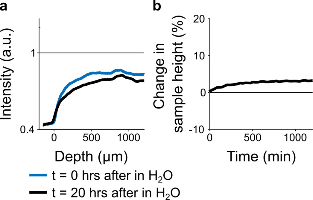
(a) Spatial intensity profile of accumulated heavy metals at the beginning t=0 hr and after t=20 hr of immersion in double distilled H2O (n=1).
Note, the slight decrease in intensity can be explained on one hand by the wash out of unbound osmium from the sample as well as by expansion of the tissue which reduces the local heavy metal density. (b) Temporal tissue expansion profile for 20 hr immersion in double distilled H2O (n=1).
Figure 2—figure supplement 4
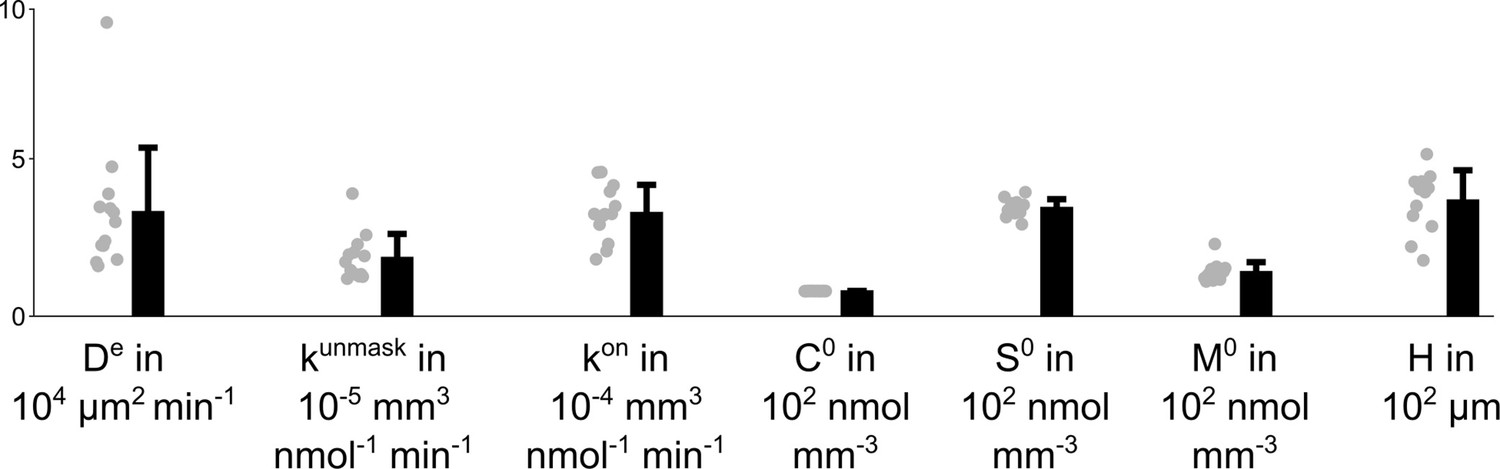
Effective diffusion coefficient De, unmasking rate constant kunmask, binding rate constant kon, the OsO4 concentration in the solution C0, the initial density of binding sites S0, the initial density of masked binding sites M0 and the sample curvature height H for n=13 different 4 mm punches that have been immersed for 22 hr in 2% buffered OsO4 solution.
The parameters have been fitted to the experimental data by simulating the model Equations 2–5; 7, while C0 has been measured for each sample individually.
Figure 2—figure supplement 5
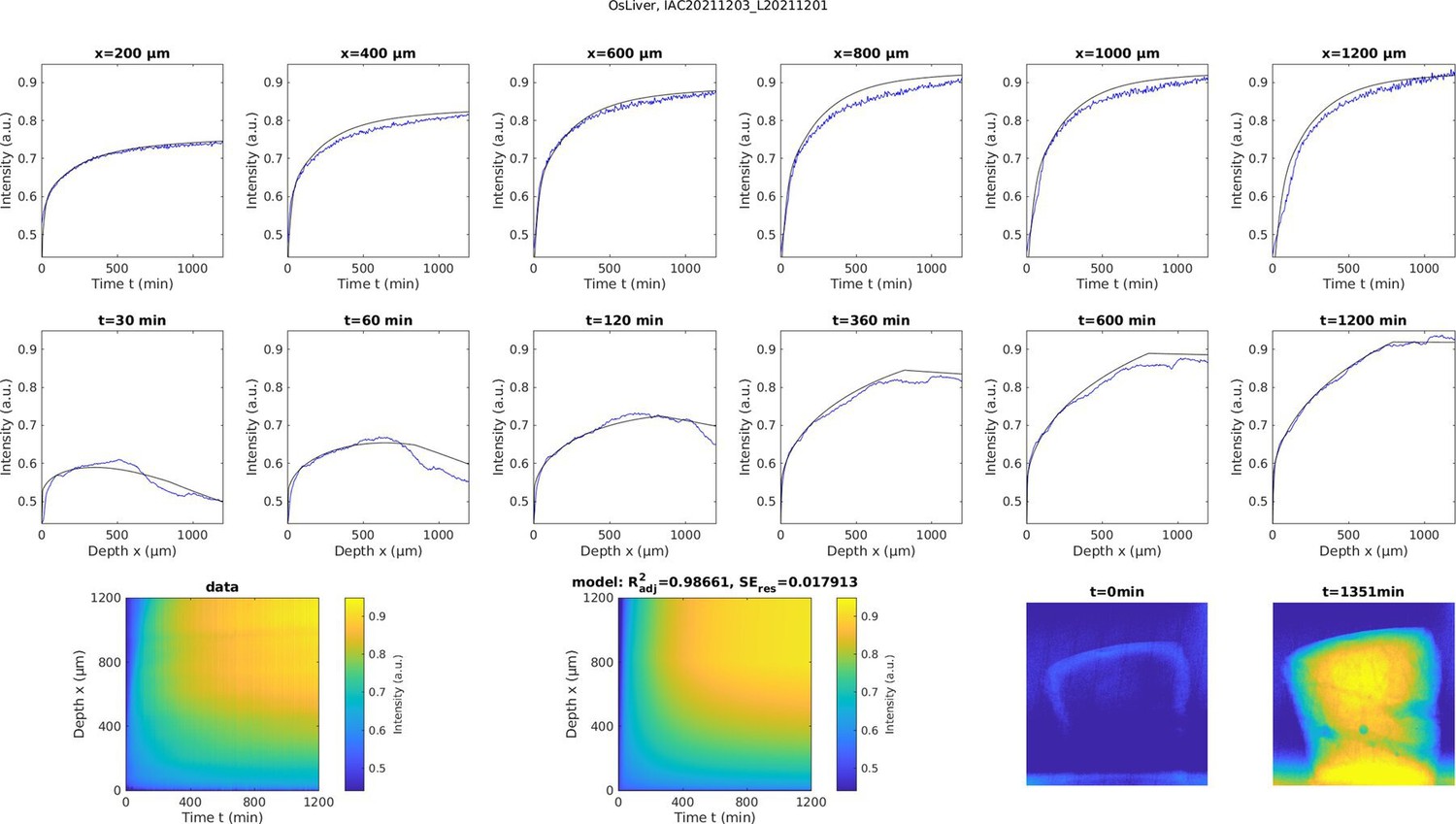
Experimentally measured accumulation of heavy metals (blue traces) in buffered 2% OsO4 solution of a 4 mm punch of aldehyde-fixed liver tissue (n=1).
The corresponding simulated model was fitted to the experimental data of the liver sample (black traces). The first row shows the temporal profile of osmium accumulation at different depths measured from the top of the sample, while the second row shows the spatial profile of osmium accumulation at different times after staining onset. The third row shows the measured spatial-temporal accumulation of osmium (left), the corresponding fitted model simulations (middle) and the distribution of osmium in projection images of the sample at the beginning of the experiment and after about 22 hr of incubation (right). The fitted model parameters were: De = 1.496·105 μm2/min, kunmask = 1.681·10–5mm3/nmol/min, kon = 2.190·10–4mm3/nmol/min, S0=2.997·102 nmol/mm3, M0=1.901·102 nmol/mm3, H=8·102 μm, C0=0.823·102 nmol/mm3. The effective diffusion coefficient appears to be >4 X larger in liver tissue compared to brain tissue. The residual standard error of the fitted model was SEres <0.018.
Additional files
Download links
A two-part list of links to download the article, or parts of the article, in various formats.
Downloads (link to download the article as PDF)
Open citations (links to open the citations from this article in various online reference manager services)
Cite this article (links to download the citations from this article in formats compatible with various reference manager tools)
In situ X-ray-assisted electron microscopy staining for large biological samples
eLife 11:e72147.
https://doi.org/10.7554/eLife.72147


