In situ X-ray-assisted electron microscopy staining for large biological samples

Version of Record

Accepted for publication after peer review and revision.

Download
Cite
Share
CommentOpen annotations (there are currently 0 annotations on this page).

528 views

Version of Record published: November 15, 2022 (This version)
Accepted Manuscript published: October 20, 2022 (Go to version)
Accepted: October 18, 2022
Received: July 13, 2021
Preprint posted: June 20, 2021 (Go to version)

1. Of interest
THINGS-data, a multimodal collection of large-scale datasets for investigating object representations in human brain and behavior

Martin N Hebart, Oliver Contier ... Chris I Baker

Tools and Resources Updated Mar 24, 2023
Further reading

Article
Figures and data
Abstract
Editor's evaluation
Introduction
Results
Discussion
Methods
Data availability
References
Decision letter
Author response
Article and author information
Metrics

Abstract

Electron microscopy of biological tissue has recently seen an unprecedented increase in imaging throughput moving the ultrastructural analysis of large tissue blocks such as whole brains into the realm of the feasible. However, homogeneous, high-quality electron microscopy staining of large biological samples is still a major challenge. To date, assessing the staining quality in electron microscopy requires running a sample through the entire staining protocol end-to-end, which can take weeks or even months for large samples, rendering protocol optimization for such samples to be inefficient. Here, we present an in situ time-lapsed X-ray-assisted staining procedure that opens the ‘black box’ of electron microscopy staining and allows observation of individual staining steps in real time. Using this novel method, we measured the accumulation of heavy metals in large tissue samples immersed in different staining solutions. We show that the measured accumulation of osmium in fixed tissue obeys empirically a quadratic dependence between the incubation time and sample size. We found that potassium ferrocyanide, a classic reducing agent for osmium tetroxide, clears the tissue after osmium staining and that the tissue expands in osmium tetroxide solution, but shrinks in potassium ferrocyanide reduced osmium solution. X-ray-assisted staining gave access to the in situ staining kinetics and allowed us to develop a diffusion-reaction-advection model that accurately simulates the measured accumulation of osmium in tissue. These are first steps towards in silico staining experiments and simulation-guided optimization of staining protocols for large samples. Hence, X-ray-assisted staining will be a useful tool for the development of reliable staining procedures for large samples such as entire brains of mice, monkeys, or humans.

Editor's evaluation

This important study explores the kinetics of heavy metal staining of tissue using time-lapse imaging with X-ray micro computed tomography (CT). Introducing a compelling approach to investigate staining in situ, this work will be of interest to the wide community of scientists preparing biological samples in particular for large-volume electron microscopy. It will become a reference for the field in establishing a quantitative tool for assessing and developing staining protocols.

https://doi.org/10.7554/eLife.72147.sa0

Introduction

In the past decade the image acquisition rates of biological electron microscopy facilities have been scaled to 10⁷–10⁹ pixels per second through parallelization and automation (Hayworth et al., 2014; Schalek et al., 2011; Ren and Kruit, 2016; Denk and Horstmann, 2004; Hayworth et al., 2020; Eberle et al., 2015; Graham et al., 2019; Xu et al., 2017). The increase in imaging throughput for biological samples has been mainly driven by the emerging Neuroscience field of connectomics which aims to densely reconstruct neuronal circuits with synaptic resolution (Briggman et al., 2011; Helmstaedter et al., 2013; Bock et al., 2011; Zheng et al., 2018; Scheffer et al., 2020; Kornfeld et al., 2017; Wanner and Friedrich, 2020; Lee et al., 2016; Kasthuri et al., 2015; Wilson et al., 2019; Schmidt et al., 2017; Svara et al., 2018; Vishwanathan et al., 2017). Also, the analysis of the terabyte-sized electron microscopy datasets produced by these studies is becoming increasingly automated using machine-learning and computer vision (Januszewski et al., 2018; Dorkenwald et al., 2020; Schubert et al., 2019; Dorkenwald et al., 2017; Berning et al., 2015; Staffler et al., 2017; Jain et al., 2010; Buhmann et al., 2020; Vergara et al., 2020; Turner et al., 2020). Both the image acquisition as well as the image analysis for these types of datasets are being scaled by parallelization to large samples on the order of several cubic millimeters or even entire brains. However, a remaining obstacle is the lack of reliable tissue processing and staining protocols for large samples where the smallest dimension is greater than 1 mm.

Existing en bloc electron microscopy staining protocols have been optimized for staining small samples with dimensions of less than 1 mm (Genoud et al., 2018; Hua et al., 2015; Deerinck et al., 2010; Tapia et al., 2012). Using aldehyde-stabilized cryopreservation (McIntyre and Fahy, 2015) the cellular ultrastructure can be preserved even in large tissue blocks with dimensions exceeding 1 mm and entire brains. Despite pioneering work on en bloc staining protocols for whole mouse brains (Mikula and Denk, 2015; Mikula et al., 2012), large en bloc stained samples still suffer from artifacts such as inhomogeneous staining and membrane or tissue cracks.

En bloc sample preparation for electron microscopy generally requires tissue fixation, staining and embedding in resin. First, the macromolecules in the tissue are stabilized via crosslinking by diffusing or perfusing buffered solutions of fixatives such as formaldehyde (Claude and Fullam, 1945; Fox et al., 1985) and glutaraldehyde (Sabatini et al., 1964). Because biological tissue is composed mostly of carbon and other low atomic number elements, the tissue is stained with heavy metals to increase the contrast in electron micrographs (Bahr, 1954; Porter et al., 1945). These heavy metal stains are composed of electron dense atoms such as osmium, lead or uranium. In addition, some of these heavy metals (e.g. osmium) also act as fixatives (Bahr, 1955). Finally, the stained tissue gets dehydrated and embedded in resin. The most commonly used resins are epoxy resins (Maaløe and Andersen, 1956), such as araldite (Glauert et al., 1956) or Epon (Finck, 1960) because of their thermal stability and electron transparency. To inspect the staining quality in an electron microscope, ultrathin sections (<100 nm) are typically collected from the embedded tissue using an ultramicrotome.

Many steps in the classic en bloc electron microscopy staining protocols are based on passive diffusion of chemicals into the tissue. Passive diffusion is one of the main bottlenecks for preparing large samples (smallest dimension >1 mm) for electron microscopy (Burkl and Schiechl, 1968; Medawar, 1941). For small samples (smallest dimension <1 mm) a typical en bloc staining protocol takes about 10–15 days including sectioning (Tapia et al., 2012). However, for large samples or whole brains, a diffusion-based staining protocol takes several weeks or even months (Mikula et al., 2012; Mikula and Denk, 2015; Masís et al., 2018).

To date, electron microscopy staining is a ‘black box’ and changes to staining protocols can only be assessed using an electron microscope, which in turn requires a sample to be run through the entire staining protocol. Conventional approaches for optimizing the parameters of staining protocols rely on sequential screening of hundreds of samples that have been processed end-to-end. However, sequential screening is very inefficient for months-long protocols.

Recently, X-ray based computed micro-tomography (μCT) has been introduced for a relatively fast, macroscopic assessment of staining quality and tissue integrity of resin-embedded whole mouse brains (Mikula and Denk, 2015; Kuan et al., 2020; Dyer et al., 2017). (Mikula and Denk, 2015) showed that the pixel intensities of serial-section EM images and the intensity of the corresponding reslice are similar. Building on this pioneering work, we developed in situ time-lapsed X-ray-assisted staining to observe the staining process while the samples are in the staining solution (Figure 1a). We used X-ray-assisted staining to explore the micro-scale tissue mechanics and the kinetics of the heavy metal diffusion and accumulation in large aldehyde-fixed brain tissue blocks, resulting in new insights on how different staining agents affect the tissue. X-ray-assisted staining opens the ‘black box’ of electron microscopy staining protocols. Each staining step can be monitored and assessed in real time. This enables in silico optimization of electron microscopy staining protocols, which will be particularly useful for the development of staining procedures for large biological samples such as whole brains (Figure 1g).

Figure 1 with 3 supplements see all

Download asset Open asset

X-ray assisted staining.

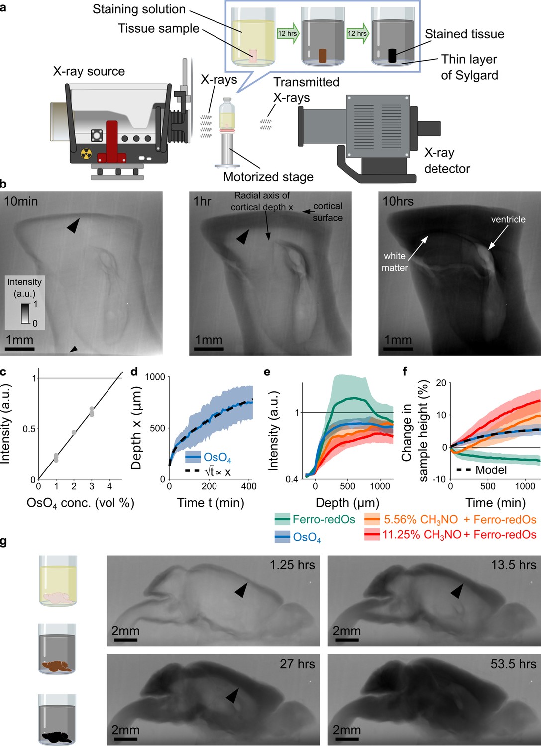
(a) Experimental setup. The sample was glued into a thin layer of Sylgard and sits in staining solution in a sealed glass vial on a motorized stage. X-rays are emitted from an X-ray source, pass through the sample, and the spatial distribution of the transmitted X-rays is detected and used to form a projection image of the X-ray absorption in the sample. Over time, the heavy metals diffuse into the tissue and the accumulation of heavy metals change the X-ray absorption properties of the sample. For the quantitative results presented in this study we used cylindrical tissue samples extracted with a 4 mm diameter biopsy punch from the cortex of mice. (b) Projection images of a 4 mm punch of mouse cortex incubated in 2% buffered osmium tetroxide (OsO₄) solution after 10 min, 1 hr, and 10 hr. The osmium diffuses passively from the cortical surface and the brain ventricles into the tissue and forms a staining front of tissue-bound osmium (large arrowhead) that moves towards the center of the sample as time progresses. The accumulation of heavy metals results in an increase in the pixel intensity (a.u.) of the X-ray projection image, which was measured along the radial axis of cortical depth from the cortical surface towards the white matter. The small arrowhead indicates the upper edge of the 2 mm thin layer of Sylgard. (c) Measured pixel intensities of the X-ray projection images for different concentrations of buffered OsO₄ solutions. The higher/darker the intensity, the more X-rays are absorbed. The pixel intensity/X-ray absorption scales linearly with the concentration/density of osmium (black line, Pearson correlation coefficient r=0.99, <10^–6; n=3 for each concentration). (d) Propagation of the staining front in 4 mm brain punches immersed in 2% buffered OsO₄ solution (n=13) measured along the radial axis of cortical depth (mean ±s.d.). The propagation can be fitted by a quadratic model (dashed black lines) in which the penetration depth x of the staining front is proportional to the square root of the incubation time t (residual standard error: SE_res = 14.68 μm). (e) Intensity profiles of the spatial heavy metal accumulation after t=20 hr of incubation in 2% buffered OsO₄ (blue, n=13), Ferro-redOs (green, n=6). Ferro-redOs with 5.56% (orange, n=4) and 11.25% formamide (red, n=4) solutions (mean ±s.d.). In Ferro-redOs the heavy metal staining is not homogenous and there is a more densely stained tissue band at a depth of 300–800 μm. (f) Tissue expansion quantified as change in sample height of aldehyde-fixed brain punches immersed in OsO₄ (blue, n=13), Ferro-redOs (green, n=6), Ferro-redOs with 5.56% (orange, n=4) and 11.25% formamide (red, n=4), respectively, as a function of the immersion duration (mean ±s.d.). All solutions were buffered by cacodylate. A monomolecular growth model was fitted to the average tissue expansion in OsO₄ solution (black dashed line, residual standard error SE_res = 0.06%). (g) In situ X-ray-assisted staining of large tissue samples. The images show projections of a whole mouse brain incubated in 2% buffered OsO₄ at different points in time across 2.5 days. The arrowheads indicate the location of the staining front of accumulated osmium. Scale bar 2 mm.

Figure 1—source data 1 Experimentally measured accumulation of heavy metals (blue traces) in buffered 2% OsO₄ solution in n=13 different samples. The corresponding simulated model was fitted individually to the experimental data of each sample (black traces). The first row of every sample shows the temporal profile of osmium accumulation at different cortical depths, while the second row shows the spatial profile of osmium accumulation at different times after staining onset. The black circles indicate the location of axon tracts that tended to accumulate osmium faster and stronger. The third row shows the measured spatial-temporal accumulation of osmium (left), the corresponding fitted model simulations (middle) and the distribution of osmium in projection images of the sample at the beginning of the experiment and after about 22 hr of incubation (right).: https://cdn.elifesciences.org/articles/72147/elife-72147-fig1-data1-v2.pdf
Download elife-72147-fig1-data1-v2.pdf
Figure 1—source data 2 Experimentally measured accumulation of heavy metals in a buffered solution of 2% OsO4 reduced with 2.5% potassium ferrocyanide K4[Fe(CN)6] (Ferro-redOs) in n=6 different samples. The first row shows the temporal profile of osmium accumulation at different cortical depths, while the second row shows the spatial profile of osmium accumulation at different times after staining onset. The black circles indicate the location of axon tracts that tended to accumulate osmium faster and stronger. The third row shows the measured spatial-temporal accumulation of osmium (left) and the corresponding distribution of osmium in projection images of the sample at the beginning of the experiment and after about 22 hoursr of incubation (right).: https://cdn.elifesciences.org/articles/72147/elife-72147-fig1-data2-v2.pdf
Download elife-72147-fig1-data2-v2.pdf
Figure 1—source data 3 Experimentally measured accumulation of heavy metals in buffered 2% Ferro-redOs solution with 5.56% formamide in n=4 different samples. The first row of every sample shows the temporal profile of osmium accumulation at different cortical depths, while the second row shows the spatial profile of osmium accumulation at different times after staining onset. The black circles indicate the location of axon tracts that tended to accumulate osmium faster and stronger. The third row shows the measured spatial-temporal accumulation of osmium (left) and the corresponding distribution of osmium in projection images of the sample at the beginning of the experiment and after about 22 hoursr of incubation (right).: https://cdn.elifesciences.org/articles/72147/elife-72147-fig1-data3-v2.pdf
Download elife-72147-fig1-data3-v2.pdf
Figure 1—source data 4 Experimentally measured accumulation of heavy metals in buffered 2% Ferro-redOs solution with 11.25% formamide in n=4 different samples. The first row of every sample shows the temporal profile of osmium accumulation at different cortical depths, while the second row shows the spatial profile of osmium accumulation at different times after staining onset. The black circles indicate the location of axon tracts that tended to accumulate osmium faster and stronger. The third row shows the measured spatial-temporal accumulation of osmium (left) and the corresponding distribution of osmium in projection images of the sample at the beginning of the experiment and after about 22 hoursr of incubation (right).: https://cdn.elifesciences.org/articles/72147/elife-72147-fig1-data4-v2.pdf
Download elife-72147-fig1-data4-v2.pdf
Figure 1—source data 5 Experimentally measured accumulation of heavy metals in a buffered solution of 2% OsO4 reduced with 2.5% potassium ferricyanide K3[Fe(CN)6] (Ferri-redOs) in n=2 different samples. The first row shows the temporal profile of osmium accumulation at different cortical depths, while the second row shows the spatial profile of osmium accumulation at different times after staining onset. The black circles indicate the location of axon tracts that tended to accumulate osmium faster and stronger. The third row shows the measured spatial-temporal accumulation of osmium (left) and the corresponding distribution of osmium in projection images of the sample at the beginning of the experiment and after about 22 hoursr of incubation (right).: https://cdn.elifesciences.org/articles/72147/elife-72147-fig1-data5-v2.pdf
Download elife-72147-fig1-data5-v2.pdf

Results

We developed in situ time-lapsed X-ray-assisted staining with the goal of facilitating and accelerating the optimization of staining protocols for large biological samples such as whole mouse brains (Abbott et al., 2020). 4mm-brain punches of transcardially perfused mice were immersed in aldehyde fixatives for 36 hr. After washing the sample blocks with cacodylate buffer, the samples were immersed in staining solution and immediately placed in the acquisition chamber of a Zeiss Xradia 520 Versa 3D for X-ray microscopy (Figure 1a). The Xradia can be operated in two different modes:

In the μCT mode, projections of the sample are acquired at different rotation angles in order to reconstruct a 3D computed tomograph of the sample. Depending on the required signal to noise and resolution, this mode allowed us to acquire approximately 1–2 computed tomographs per hour.
In single-projection mode, a projection of the sample is acquired in a fixed position every few seconds without rotating the sample.

The advantage of the μCT mode is that arbitrary virtual reslices can be extracted to assess the staining progression in various parts of the sample. However, with our X-ray microscope, the temporal resolution in μCT mode was limited to 30–60 min per tomograph. Therefore we performed all quantitative experiments in single-projection mode where the temporal resolution for monitoring of the heavy metal diffusion and accumulation was on the order of a few seconds. Note, in this mode, the pixel intensities of the resulting X-ray projection images are accumulated through the entire sample and therefore the correspondence to the pixel intensities in thin serial-section EM images is less accurate than in μCT mode (Figure 1—figure supplement 1). As soon as the samples got placed in the staining solutions, the heavy metals started accumulating in the immersed tissue. The stained tissue absorbs more X-rays than the unstained tissue, resulting in a noticeable intensity difference that can be used to track the diffusion and accumulation of the heavy metals in the tissue (Figure 1b).

Quadratic scaling of incubation times with sample size

Osmium tetroxide (OsO₄) is one of the most commonly used contrast agents for lipid staining in electron microscopy due to its large atomic number and its ability to integrate into cellular membranes (Porter et al., 1945; Palade, 1952; Watson, 1958). The immersion times for OsO₄ vary between a few minutes to several days, depending on the sample size and tissue type, and are usually determined empirically (Genoud et al., 2018; Hua et al., 2015; Tapia et al., 2012; Mikula and Denk, 2015). However, the kinetics of OsO₄ staining of biological tissue are not well understood and so far had to be determined experimentally by trial and error. We therefore set out to measure the diffusion and accumulation of OsO₄ by placing 4 mm punches of aldehyde-fixed mouse brains in 2% buffered OsO₄ solution. The osmium diffused into the tissue and accumulated in the sample during the staining process (Figure 1b). The intensity of X-ray absorption in the projection images scales linearly with the local concentration/density of osmium (Figure 1c). The density of OsO₄ in the tissue increased beyond the density in the surrounding staining solution, indicating that the density of binding sites for OsO₄ in the tissue is higher than the concentration of the OsO₄ in the staining solution (Figure 1b). The diffusion and spatio-temporal accumulation of OsO₄ results in a staining front that propagates towards the center of the sample (Figure 1b). As expected for diffusive processes (Carnevale et al., 1979), the propagation of the OsO₄ staining front can be approximated by a quadratic model (Figure 1d). As in the case of other fixatives (Medawar, 1941), the osmium staining penetration in aldehyde fixed tissue obeys a quadratic scaling law, or rather a “rule of thumb”, for how the necessary incubation time t depends on the staining depth or sample size x:

t \propto x^{2}

This means, for example, that if one would adapt an established OsO₄ staining protocol for 3 X larger samples, one would have to prolong the incubation time by 9 X in order to produce comparable staining results. Similarly, the time it takes for any point in the sample to reach a given concentration is proportional to the square of its distance to the sample surface (Carnevale et al., 1979).

Monitoring staining kinetics and tissue deformation

After 20 hr of incubation the staining density of osmium is homogeneous across the first 1000 μm of cortical depth (Figure 1e). In addition, the ultrastructure is well preserved (Figure 1—figure supplement 2). Reduced osmium is another commonly used staining agent that is known to result in higher contrast for electron microscopy images than non-reduced OsO₄. Typically, a buffered 2% OsO₄ solution is reduced with 2.5% potassium ferrocyanide (K₄[Fe(CN)₆]) (Hua et al., 2015; Willingham and Rutherford, 1984; Mikula and Denk, 2015), which we will call Ferro-redOs throughout this manuscript. Consistent with previous reports on Ferro-redOs staining in large samples (Hua et al., 2015; Mikula and Denk, 2015) we found that for Ferro-redOs the accumulation of heavy metals peaks at a depth between 300 and 800 μm (Figure 1e), whereas the tissue above or below that depth is stained less. Traditionally, this band of more heavily stained tissue has been associated with precipitated osmium that hinders the diffusion and prevents homogenous staining (Genoud et al., 2018; Hua et al., 2015; Mikula and Denk, 2015), in particular deeper in the tissue. No such band is present in tissue immersed in non-reduced OsO₄. (Mikula and Denk, 2015) reported that homogeneous staining of large samples with Ferro-redOs was achieved by adding formamide to the Ferro-redOs solution. However, the underlying mechanisms by which formamide acts are not known (Mikula and Denk, 2015; Genoud et al., 2018). (Mikula and Denk, 2015) hypothesized that formamide might prevent precipitation by generally solubilizing compounds or that it might allow highly charged molecules to cross membranes more easily. Adding formamide to the Ferro-redOs solution indeed resulted in more homogeneous staining (Figure 1e, ), but the heavy metal density was lower than in osmium only. (Mikula and Denk, 2015) reported that the tissue tends to expand at high concentrations of formamide (>50%). But we found that the tissue expands even at lower formamide concentrations, while the amount of expansion depends on both the formamide concentration and the incubation duration (Figure 1f). For a concentration of 11.25% formamide, the sample height increased by about 15% within 20 hr of incubation, whereas for a formamide concentration of 5.56%, the tissue height expanded only by approximately 10% (Figure 1f). Note, in the first 3 hr of incubation in Ferro-redOs with 5.56% formamide the tissue actually shrank, suggesting that there are opposite forces acting on the tissue. Indeed, in Ferro-redOs solution without any formamide, the tissue shrank by about 5% in height (Figure 1f). In contrast, we found that in 2% buffered OsO₄ solution the sample height expands by about 5% (Figure 1f). However, we found no sample expansion if the reduced osmium solution was prepared with 2.5% potassium ferricyanide K₃[Fe(CN)₆]+ 8 a,b), another commonly used reducing agent for OsO₄.

Hua et al., 2015 suggested an alternative approach to achieve homogeneous staining in 1 mm brain punches with Ferro-redOs without formamide, in which osmium and the reducing agent are applied separately. First, the samples are immersed in buffered 2% OsO₄ solution for 90 min. Subsequently, the samples are placed for 90 min in buffered 2.5% K₄[Fe(CN)₆] without any washing step in-between. We repeated this procedure for 4 mm brain punches: First, the samples were incubated in 2% buffered OsO₄ for 22 hours resulting in homogeneous staining throughout the sample. Next, we placed the sample directly without any washing step in 2.5% buffered K₄[Fe(CN)₆] solution. (Hua et al., 2015) hypothesized that the main effect of reducing agents such as K₄[Fe(CN)₆] is to convert VIII-oxidized water-soluble osmium into an VI-oxidized water-soluble form which is thought to generate additional, non-polar OsO₂ to be deposited in the membrane increasing the heavy metal content and the contrast in electron microscopy. However, we found that the heavy metal density in the K₄[Fe(CN)₆] immersed samples did not increase, but rather decrease from the sample surface towards the center as time progressed (Figure 2a). This suggests that K₄[Fe(CN)₆] removes or “washes out” osmium from the sample (Litman and Barrnett, 1972) resulting in an inverse staining gradient. This “washing effect” is stronger for longer incubation times as well as close to the sample surface and around blood vessels (anecdotal observation in electron microscopy images, data not shown). For incubation times longer than 12 hr, K₄[Fe(CN)₆] readily dissolves and disintegrates the tissue (Figure 2—figure supplement 1). Interestingly, no ‘washing effect’ was observed if the same procedure was repeated with 2.5% potassium ferricyanide K₃[Fe(CN)₆], but the sample height shrank by about 2% (Figure 1—figure supplement 3,f, ). Similarly, only a small reduction in heavy metal density could be observed when the sample was washed with double-distilled H₂O for 20 hr (Figure 2—figure supplements 2 and 3).

Figure 2 with 5 supplements see all

Download asset Open asset

Kinetics and tissue mechanics of electron microscopy staining.

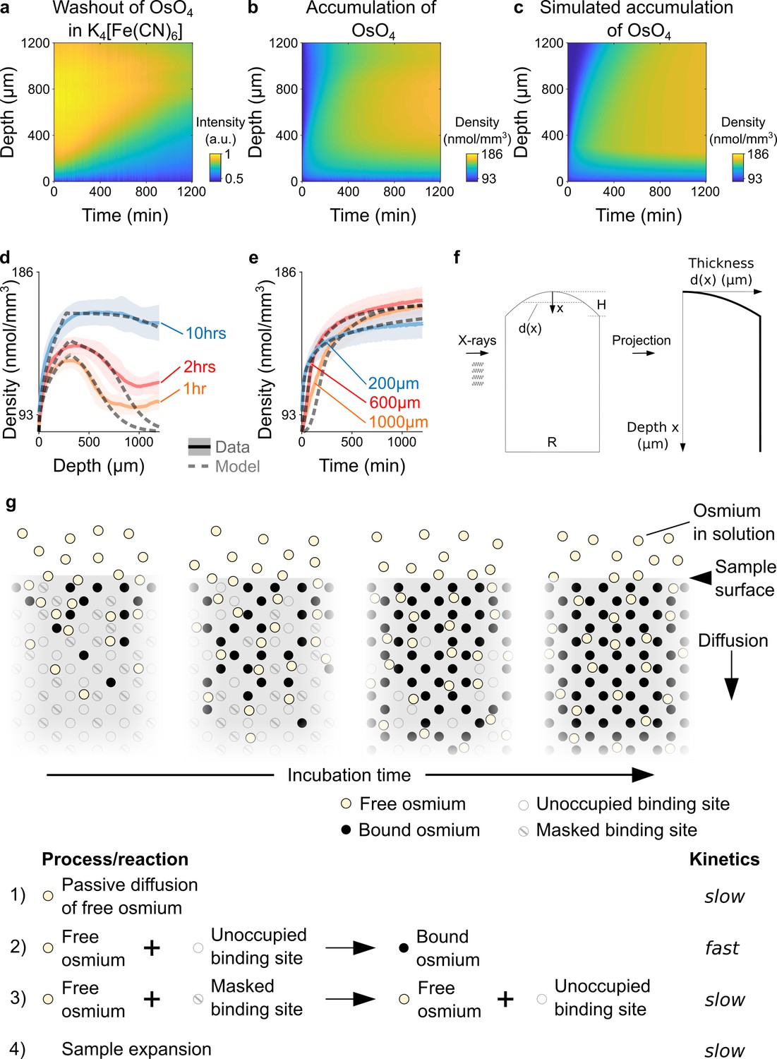
(a) Spatio-temporal washout of osmium in samples incubated in 2.5% potassium ferrocyanide K₄[Fe(CN)₆] (n=6). The samples have been stained with 2% OsO₄ for 22 hrs prior to placing them in K₄[Fe(CN)₆]. The osmium gets washed out from the sample surface towards the center as the incubation time increases. (b) Average experimentally measured spatio-temporal osmium density (nmol/mm³) accumulation in samples (n=13) immersed in 2% buffered OsO₄ solution. Because of the surface curvature of the cortical samples, the tissue thickness decreases towards the surface (x=0) and results in a lower intensity in the projection images (see tissue geometry model in f). (c) Simulated spatio-temporal osmium density (nmol/mm³) accumulation fitted to the average experimental data in b. (d) Density profiles (nmol/mm³) of the spatial accumulation of osmium (n=13, mean ±s.d.) after 1 hr (orange), 2 hrs (red), and 10 hr (blue) of incubation in 2% buffered OsO₄ overlaid with the simulation of the diffusion-reaction-advection model (dashed lines). (e) Density profiles (nmol/mm³) of the temporal accumulation of osmium (n=13, mean ±s.d.) at a depth of 200 μm (blue), 600 μm (red), and 1000 μm (orange) during incubation in 2% buffered OsO₄, overlaid with the simulation of the diffusion-reaction-advection model (dashed lines). (f) The geometry of the 4 mm brain punches was modeled as a cylinder with a curved surface. The curvature of the sample surface is approximated by a circle with radius $\frac{1}{2 H} \cdot (H^{2} + {\frac{1}{4} R}^{2})$ , where $R$ is diameter of the cylinder and $H$ is the height of the curved surface. The projected tissue thickness as a function of the depth x from the sample surface is then given by $d (x)$ : $d (x) = 2 \cdot \sqrt{\frac{x}{H} \cdot (H^{2} + {\frac{1}{4} R}^{2}) - x^{2}}$ , for $0 \leq x \leq H$ and $d (x) = R$ , for $x > H$ (g) Diffusion-reaction-advection model for osmium staining. The model combines four coupled processes: (1) Free OsO₄ diffuses passively into the tissue and (2) binds to the available binding sites. (3) In the presence of freely diffusing OsO₄ previously masked binding sites are slowly turned into additional binding sites for OsO₄. (4) The sample expands by about 5% in sample height within 20 hr of incubation (see Figure 1f).

Figure 2—source data 1 Experimentally measured washout of heavy metals in buffered 2.5% potassium ferrocyanide K₄[Fe(CN)₆] solution in n=6 different samples that have previously been stained with buffered OsO₄ for 22 hr. The first row of every sample shows the temporal profile of osmium washout at different cortical depths, while the second row shows the spatial profile of osmium washout at different times after staining onset. The black circles indicate the location of axon tracts. The third row shows the measured spatial-temporal washout of osmium (left) and the corresponding distribution of osmium in projection images of the sample at the beginning of the experiment and after about 22 hr of incubation (right).: https://cdn.elifesciences.org/articles/72147/elife-72147-fig2-data1-v2.pdf
Download elife-72147-fig2-data1-v2.pdf
Figure 2—source data 2 Experimentally measured washout of heavy metals in buffered 2.5% potassium ferricyanide K3[Fe(CN)6] solution in n=4 different samples that have previously been stained with buffered OsO4 for 22 hrs. The first row of every sample shows the temporal profile of osmium washout at different cortical depths, while the second row shows the spatial profile of osmium washout at different times after staining onset. The black circles indicate the location of axon tracts. The third row shows the measured spatial-temporal washout of osmium (left) and the corresponding distribution of osmium in projection images of the sample at the beginning of the experiment and after about 22 hoursr of incubation (right).: https://cdn.elifesciences.org/articles/72147/elife-72147-fig2-data2-v2.pdf
Download elife-72147-fig2-data2-v2.pdf

The kinetics of osmium tetroxide staining

The chemistry and diffusion-reaction-advection kinetics of OsO₄ staining in aldehyde-fixed tissue are not well understood. In brain tissue, OsO₄ is thought to mainly react with carbon-carbon double bonds, in particular of unsaturated lipids, but it has also been reported to react with some amino acids and nucleotides (Khan et al., 1961; Korn, 1967; White et al., 1976; Schroeder, 1980). At the beginning of the OsO₄ incubation, the density of OsO₄ steeply increases and peaks close to the surface of the sample. As the incubation time progresses, the OsO₄ continues to diffuse and accumulates deeper in the tissue (Figure 2b, d and e). Due to the curved surface of the cortical tissue sample, the projected tissue thickness is lower (Figure 2f) and there are fewer binding sites for osmium, which results in a lower density of osmium closer to the sample surface (Figure 2b). At any given time, the accumulation seems to plateau from the surface towards the center of the sample, indicating that the binding of OsO₄ saturates (Figure 2d and e). However, we found that the saturated density in the samples slowly increased over time from about 129 nmol/mm³ after 1 hr of incubation to 160 nmol/mm³ after 10 hr of incubation (Figure 2b, d and e), while the density of the solution remained stable at about 82 nmol/mm³. This suggests that additional binding sites for OsO₄ become available slowly over time. The reactions underlying the ‘unmasking’ of binding sites are not known, but we hypothesize that it depends at least partially on the availability and the local concentration of unbound, freely diffusing osmium. Hence, at the macroscale level, the accumulation of osmium in biological tissue can be described by four coupled processes (Figure 2g): As the osmium diffuses passively into the tissue, it binds to the available binding sites in the tissue and additional binding sites are slowly being unmasked, while the tissue expands by around 5% within 20 hr of incubation (Figure 1f). The kinetics of these four processes can be described with the following coupled (non-linear) partial differential equations:

\begin{matrix} \frac{\partial f (x, t)}{\partial t} = D^{e} \cdot \frac{\partial^{2} f (x, t)}{\partial x^{2}} - k^{o n} \cdot s (x, t) \cdot f (x, t) & - \frac{\partial}{\partial x} [f (x, t) \cdot v (x, t)] \end{matrix}

\begin{matrix} \frac{\partial b (x, t)}{\partial t} = k^{o n} \cdot s (x, t) \cdot f (x, t) & - \frac{\partial}{\partial x} [b (x, t) \cdot v (x, t)] \end{matrix}

\begin{matrix} \frac{\partial s (x, t)}{\partial t} = - k^{o n} \cdot s (x, t) \cdot f (x, t) + k^{u n m a s k} \cdot m (x, t) \cdot f (x, t) & - \frac{\partial}{\partial x} [s (x, t) \cdot v (x, t)] \end{matrix}

\begin{matrix} \frac{\partial m (x, t)}{\partial t} = - k^{u n m a s k} \cdot m (x, t) \cdot f (x, t) & - \frac{\partial}{\partial x} [m (x, t) \cdot v (x, t)] \end{matrix}

f(x,t) is the density of freely diffusing OsO₄, b(x,t) is the density of osmium bound to the tissue, s(x,t) is the density of available binding sites and m(x,t) corresponds to the density of masked binding sites at time t and a radial depth x from the cortical surface. D^e is the effective diffusion coefficient for OsO₄, k^on is the reaction rate constant for the binding of osmium to the tissue and k^unmask is the reaction rate constant at which masked binding sites get unmasked. In addition, the local change of the tissue geometry, e.g. the expansion as observed for OsO₄, results in a velocity field v(x,t) that describes the local spatio-temporal flow of the density of each component c(x,t):

\frac{\partial}{\partial x} [c (x, t) \cdot v (x, t)] = \frac{\partial c (x, t)}{\partial x} \cdot v (x, t) + c (x, t) \cdot \frac{\partial v (x, t)}{\partial x}

The flow consists of an advection term $\frac{\partial c (x, t)}{\partial x} \cdot v (x, t)$ , corresponding to elemental volumes moving with the local flow, and a dilution term $c (x, t) \cdot \frac{\partial v (x, t)}{\partial x}$ that describes the local volume change. While we assume that the tissue density is homogeneous across the cortical thickness, we consider differences in the sample thickness due to the curvature of the cortical surface. Additional information on the model assumptions can be found in the methods section.

We fitted the parameters of the system of reaction-diffusion-advection equations for a tissue sample with the projection geometry shown in Figure 2f to the average measured spatio-temporal accumulation of OsO₄ (Figure 2b–e) as well as to the individual samples (n=13, ). The fitted parameters of the diffusion-reaction-advection model (Figure 2—figure supplement 4) capture the measured diffusion-reaction-advection kinetics of osmium staining well (Figure 2c; residual standard error SE_res = 0.026 ± 0.005, mean ±s.d.).

Discussion

In situ X-ray-assisted staining is a new tool for monitoring the different steps of en bloc staining protocols for electron microscopy. By opening the ‘black box’ of staining protocols, X-ray-assisted staining enables, for the first time, to observe directly the diffusion of heavy metals and their microscopic effects on the tissue. While the technique will be useful to develop novel staining protocols for small to intermediate sized samples with dimensions less than 1 mm, it will particularly accelerate and facilitate the development and optimization of new staining protocols for large biological samples such as whole brains (Figure 1g).

We monitored the accumulation of osmium in different commonly used staining solutions and found significant differences in the accumulation densities. In addition, we found that the tissue expands and shrinks significantly depending on the composition of the staining solution. In particular, we found that the tissue height increased by 5% in buffered osmium solution, while the tissue height decreased by 5% in buffered Ferro-redOs solution. We hypothesize that this shrinkage could provide a mechanistic explanation for the long standing issue of diffusion barrier formation in large samples during Ferro-redOs incubation.

The method also revealed that K₄[Fe(CN)₆], a reducing agent that was believed to enhance the accumulation of osmium in membranes, in contrast can wash out osmium from stained tissue if applied separately. If K₄[Fe(CN)₆] removes osmium from the sample, why does the protocol modification of Hua et al., 2015 result in enhanced electron microscopy contrast for samples with dimensions of up to 1 mm? A potential explanation could be that K₄[Fe(CN)₆] clears the cytosol more efficiently than the cell membranes. As a consequence, the osmium content in the cytosol gets washed out more/faster, which might result in an overall electron microscopic contrast increase between the membranes and the cytosol. However, the chemical mechanisms by which K₄[Fe(CN)₆] interact with the tissue remain poorly understood and shining a light on those processes will require additional work.

X-ray assisted staining opens the door for in silico staining protocol optimization, by enabling to measure important heavy metal staining parameters such as the effective diffusion coefficients and reaction rate constants directly in situ. We derived a diffusion-reaction-advection model that describes the accumulation of osmium in homogeneous tissue by four distinct, but coupled, processes. Osmium diffuses passively into the tissue and binds there quickly to available binding sites, for example unsaturated lipids. Thereby the tissue expands by about 5% in height. Additional binding sites are being unmasked over the course of hours, which enables the tissue to accumulate additional osmium. While the binding of osmium appears to be nearly instantaneous, the passive diffusion and unmasking reactions are slow and appear to be rate-limiting for the staining. The mechanisms and reactions underlying the unmasking of additional binding sites for osmium are not known. Unsaturated lipids, one of the prominent binding sites for osmium, can be masked by lipid-protein complexes. In the presence of osmium, these complexes could dissociate and make the previously masked unsaturated lipid available for binding osmium (Clayton, 1959; Lauder and Beynon, 1993; Ashhurst, 1961; Wigglesworth, 1975). A recent study used time-of-flight secondary ion mass spectrometry to analyze the colocalization of different fatty acid species with osmium at the tissue surface (Belazi et al., 2009). As expected, the unsaturated fatty acids colocalize well with the tissue-bound osmium. However, they also report a remarkable complementary clustering of saturated and unsaturated fatty acids in osmium stained tissue that appears not to be present in unstained tissue. Hence, it could be that osmium can convert saturated lipids to unsaturated lipids through hydrogenation/oxidation. Alternatively, the masked binding sites could also be interpreted as a different binding partner that reacts much slower with osmium.

Biological samples such as brains are non-homogeneous media. They are composed of different tissue and cell types and therefore the diffusion of staining agents is expected to be heterogeneous. Nevertheless, the fitted model parameters reproduce the observed kinetics of osmium accumulation relatively well up to a depth of about 700–800 μm from the surface. Deeper in the tissue osmium that diffused from secondary sources such as ventricles or axon tracts appear to contribute to the accumulation of osmium. For example, we found that white matter and myelinated axon tracks tend to accumulate osmium faster and stronger compared to gray matter (, ). Such secondary sources and tissue inhomogeneities are not considered in our model. Still, the fitted model parameters appear consistent with comparable values from the literature, although we also find some discrepancies. For example, in mouse brains we expect to find about 117.975 nmol/mm³ double-bonds on unsaturated lipids (see methods for the derivation). Because the dominant binding reaction for osmium is assumed to be the formation of mono- and di-ester bonds with unsaturated lipids which has been described to result in the deposition of OsO₂, the density of double bonds should roughly correspond to the density of available binding sites. But the proposed model predicts 2.999 times more binding sites, even without unmasking. One interpretation would be that unsaturated lipids are not the dominant reaction partner and that other reaction partners such particular amino acids or nucleotides account for about two third of the available binding sites. Alternatively, this could indicate that each unsaturated lipid double bond gets associated with on average 3 osmium atoms, for example through Os₃O₅^- and Os₃O₅H^- isotopes that have previously reported to exist in osmium-stained adipose mouse tissue (Belazi et al., 2009). Similarly, it has been reported that if the mono- and di-ester products are left standing in solution, a highly insoluble trimer osmium product is formed (Schroeder, 1980).

We expect that X-ray-assisted staining will be very useful in establishing a more refined picture of the heterogeneity of the heavy metal diffusion processes in different tissue types and compartments as well as in different conditions. For example, we also measured and modeled the accumulation of osmium in liver tissue (Figure 2—figure supplement 5). It will also be interesting to examine how changes in the extracellular space and different fixation protocols or microwave-assisted incubation affect the diffusion dynamics (Korogod et al., 2015; Fulton and Briggman, 2020; Jensen and Harris, 1989; Login and Dvorak, 1988).

Furthermore, X-ray-assisted staining can be used at higher resolution and in combination with computed tomography for producing a more detailed picture of the tissue mechanics involved in different staining steps. We and several other labs have noticed that brain tissue expands significantly during incubation in ‘osmium amplifiers’ such as the osmiophilic thiocarbohydrazide (TCH) (Seligman et al., 1966). (Mikula and Denk, 2015) reported that nitrogen bubbles are formed during TCH incubation that could be responsible for the formation of tissue cracks in large samples. X-ray-assisted staining could be used to detect and monitor the formation of tissue cracks and to explore ways to reduce these artifacts in large samples.

Aside from accelerating the development of novel staining protocols this new method will also allow for improved closed-loop quality control of the staining process. Large samples tend to be biologically more variable and more difficult to precisely fine-tune all the parameters in the staining protocol ahead of time to account for these individual differences. Hence, X-ray-assisted staining can be used to adjust the parameters in real time to compensate for these individual differences. This is particularly important for experiments in which the sample yield is low or the individual sample is precious, as for example in the case of human brains or functionally imaged brains of behaving animals that require several months of behavioral training. However, this will require calibrating what is measured with X-ray microscopy to the corresponding appearance at an electron microscopic level, because the image formation process and the resulting contrast, signal-to-noise, etc. for both imaging modalities depend not only on the staining protocol, but also on the imaging modality, energy, flux, etc. (Du and Jacobsen, 2018).

Methods

Sample preparation

Animal use procedures were approved by the Princeton University Institutional Animal Care and Use Committee (protocol number 2000) and carried out in accordance with National Institutes of Health standards (AAALAC International Institutional Number: Unit #1001, PHS assurance ID D16-00273). The experiments were carried out with C57BL/6 J mice (Jackson Laboratories, Bar Harbor, Maine, USA) of both sexes, age ranging from 13 to 58 weeks (mean ± sd: 27±9 weeks). Prior to tissue sample extraction, the mice were anesthetized by isoflurane inhalation (4%) and euthanized with an intraperitoneal injection of a ketamine (100 mg/kg) and xylazine (10 mg/kg) overdose. Next, the animals were perfused transcardially with ≥50 ml fixative solution (1.3–1.5% glutaraldehyde (GA) and 2.5–2.6% paraformaldehyde (PFA) in 0.14–0.15 M cacodylate buffer with 2.0–2.1 mM CaCl₂ at pH 7.4; (GA, PFA) and cacodylate buffer Electron Microscopy Sciences, Hatfield, PA; CaCl₂, Sigma Aldrich, St. Louis, MO). After perfusion, the animal was left for 15–60 min on ice. Subsequently, the brain was removed in order to extract tissue samples at the center of the cortical surface of each hemisphere using biopsy punches of 4 mm diameter. The liver tissue was extracted with a 4 mm biopsy punch from the center of the liver after perfusion. The samples were kept in fixative solution at 4 °C for 36 hr (4 mm biopsy punches) or for 12 hr (whole mouse brain). Next, the samples were washed 6–7 times for 30 min in 0.15 M cacodylate buffer with 2 mM CaCl₂.

Glass vials were prepared prior to the experiments with a 1–2 mm layer of Sylgard 184 (Electron Microscopy Sciences, Hatfield, PA) at the bottom. The whole mouse brain was glued with a small drop of Vetbond tissue adhesive (3 M, Hanna Pharmaceutical Supply Co., Inc, Wilmington, DE) to the bottom of the vial. For the 4 mm biopsy punch samples, a hole with a diameter of 4 mm was cut out of the Sylgard layer. Next, the samples were placed into the sylgard hole and were glued to the bottom of the glass vial with a small drop of Vetbond tissue adhesive. Subsequently, the samples were immersed in fresh cacodylate buffer solution for the transfer to the X-ray microscope. At the microscope, presets (see X-ray microscopy section below) were loaded for image acquisition. After that the washing solution was replaced with the staining solution and the sample was placed into the X-ray microscope. The acquisition of X-ray images was typically started within 5.66±2.35 min. (mean ±s.d.) after adding the staining solution. The following staining solutions have been assessed at room temperature for this study (all buffered with 0.15 M cacodylate buffer and 2 mM CaCl₂):

Osmium tetroxide: 1%, 2% and 3% OsO₄ (prepared from 2 mL 4% osmium tetroxide solution, Electron Microscopy Sciences, Hatfield, PA)
Potassium ferrocyanide: 2.5% potassium ferrocyanide (prepared from crystalline 25 g potassium hexacyanoferrate(II) trihydrate powder, Sigma Aldrich, St. Louis, MO)
Ferro-redOs: 2% OsO₄, 2.5% potassium ferrocyanide
Ferro-redOs in 11.25% formamide: 2% OsO₄, 2.5% potassium ferrocyanide, 11.25% formamide (prepared from 25 mL formamide solution, Sigma Aldrich, St. Louis, MO)
Ferro-redOs in 5.56% formamide: 2% OsO₄, 2.5% potassium ferrocyanide, 5.56% formamide
Potassium ferricyanide: 2.5% potassium ferricyanide (EMS #13746-66-2)
Potassium ferricyanide reduced osmium: 2% OsO₄, 2.5% potassium ferricyanide

Sample embedding, sectioning, and electron microscopy

After staining, the samples were washed with double-distilled H₂O 3 times for 30 min. Next, the tissue was dehydrated with iteratively increasing concentrations of ethanol (EtOH, 200 proof, anhydrous,≥99.5%, Sigma Aldrich, St. Louis, MO) in double-distilled H₂O for 30 min per step: 25% EtOH, 50% EtOH, 75% EtOH, 90% EtOH, 95% EtOH, 100% EtOH, 100% EtOH. Subsequently, the samples were transferred to 100% acetonitrile (ACS grade, Electron Microscopy Sciences, Hatfield, PA) for two 30-min washes. The tissue was embedded in hard Epon in an iterative concentration series: 1:2 Epon: acetonitrile for 12 hr, 1:1 Epon: acetonitrile for 24 hr, 2:1 Epon: acetonitrile for 2 days with fresh resin every 8–12 hr. Finally, the sample was left on the bench at room temperature for 6 days, with fresh resin every 8–12 hr, before it was placed in a 60 °C oven for curing for 5–7 days.

Serial sections of ~40 nm thickness were collected using an UC7 ultramicrotome from Leica. To assess the ultrastructural preservation of the tissue, the sections were imaged with a Zeiss Sigma SEM (Zeiss Microscopy, Oberkochen, Germany) with a backscattered electron detector (BSD) and the following acquisition parameters: 38 μs dwell time, 4 nm pixel size, probe current 200 nA, EHT voltage 6 kV, BSD Gain = High, all sectors of the detector ON.

X-ray microscopy

All X-ray microscopy experiments were performed on a Zeiss Xradia 520 Versa 3D X-ray microscope (Zeiss, Thornwood, NY). The samples were immersed in heavy metal solution in glass containers tightly sealed with Parafilm (Bemis Company, Inc, Neenah, WI) just before being placed in the recording chamber of the Xradia. Test images were acquired to check imaging parameters. For the biopsy punch samples, projections at a fixed view angle (rotation angle step size = 0°) were taken every 22–60 s resulting in about 1300–1350 images per sample over 22 hr of continuous acquisition. For the whole mouse brain, projections were taken every 22–60 s and after each projection the sample was rotated by 1°. All images were acquired using the image acquisition software Scout-and-Scan Control System (Zeiss, Thornwood, NY) with the following parameters:

Objective: 0.4 X
Tube Voltage = 100 kV
Output power = 7 W
Source filter = air (no filter)
Exposure time = 20 s.
Effective pixel size = 2–3 μm (biopsy punches) and 13–14 μm (whole mouse brain)

Image preprocessing

First, the individual images and metadata of each projection of each sample were extracted from the proprietary *.txrm and *.xrm files as saved by the Xradia image acquisition software. In addition, a time stamp of the acquisition time point was extracted from the image metadata for each projection. A custom cross-correlation based image alignment procedure (Wanner et al., 2016) was used to correct for translational offsets between images of subsequent time points. The projection images were flat-field corrected to account for radial intensity variations due to the cone-shaped X-ray beam as follows:

For each sample, a median image ${i m}_{m e d i a n}$ was calculated from the 2nd to 5th projection images right after acquisition onset.
The following quadratic 2d function was fitted to $l o g ({i m}_{m e d i a n})$ using the built-in function lsqcurvefit in MATLAB:
- $Z (x, y) = b_{5} {\cdot x}^{2} + b_{4} {\cdot y}^{2} + b_{3} {\cdot x}^{} + b_{2} \cdot y + b_{1}$
At each time t, the projection image was flat-field corrected using $Z (x, y)$ with the fitted parameters:
- ${\hat{i m}}_{t} (x, y) = \frac{i m_{t} (x, y)}{e x p (Z (x, y))} \cdot m a x (e x p (Z))$

Measuring the X-ray absorption and local heavy metal density

The pixel intensities of the detected absorbed X-rays were used as a proxy for the density of heavy metal accumulation in the tissue. In each sample, we quantified the pixel intensities in each projection taken at time t along a cross-section that pointed from the cortical surface radially towards the white matter (Figure 1b). The cross-sections were manually selected such that they started at a well detectable surface boundary and they were located at least 1 mm away from the vertical sample borders. For each sample i, the intensity $w_{i} (x, t)$ of the transmitted X-rays was quantified by averaging the pixel intensity of the cross-section at a depth $x$ at time $t$ within a width of ±25 pixels perpendicular to the axis of the cross-section. x=0 corresponds to the cortical surface of the brain samples or the surface of the liver for the liver samples. The intensity of X-ray absorption was defined as $u_{i} (x, t) = 10,000 - w_{i} (x, t)$ . For each time point t, the baseline intensity $b_{i} (t)$ was calculated by averaging the pixels outside of the sample within –50 μm and –150 μm from the sample surface along the cross-section within a width of ±25 pixels perpendicular to the axis of the cross-section. To account for baseline fluctuation in the staining solution and the X-ray illumination the intensity of X-ray absorption was baseline-corrected by $u_{i}^{b} (x, t) = u_{i} (x, t) - (b_{i} (t) - m e d i a n (b_{i}))$ .

To standardize $u_{i}^{b} (x, t)$ , the following quantities where calculated for each sample:

$\underline{b_{i}} = m e a n (u_{i}^{b} (x, t))$ was calculated for all pixels along the cross-section outside of the sample within 0 μm and –200 μm from the sample surface.
$u_{i}^{m i n} = \underline{b_{i}} - \frac{1 - 0.9}{0.9} (m - \underline{b_{i}})$
$u_{i}^{r e f} = u_{i}^{m i n} - a \cdot (m - u_{i}^{m i n})$
$u_{i}^{n o r m} = (1 + a) \cdot (m - u_{i}^{m i n})$

Finally, $u_{i}^{b} (x, t)$ was standardized to ${\hat{u}}_{i} (x, t) = (u_{i}^{b} (x, t) - u_{i}^{r e f}) / u_{i}^{n o r m}$ .

This procedure ensures that the origin is at 0 for the linear relationship between the X-ray absorption intensities in the projection images and the different OsO₄ concentrations as shown in Figure 1c and that a pixel intensity of 0.9 roughly corresponds to the saturated staining in 2% OsO₄. For this, the factors $a = 0.61749$ and $m = 6420$ were determined empirically.

Measuring the linear relationship between X-ray absorption and OsO₄ concentration

The X-ray absorption/pixel intensity of cacodylate-buffered solutions with 1%, 2% and 3% OsO₄ was measured the same way as for the X-ray absorption in stained tissue.

Monitoring of tissue expansion and shrinkage

Intensity based heuristics were used in a semi-automated procedure to detect the cortical surface in each image of each sample. The glass vial bottom was used as a reference point to measure the distance to the cortical surface $H (t)$ at time $t$ . Right after placing the samples in the X-ray the height of the samples was $H_{0} = H (t = 0)$ and the change in sample height (expansion or shrinkage) was quantified as $\frac{H (t) - H_{0}}{H_{0}} \cdot 100 %$ .

Tissue expansion modeling

The expansion of the tissue in buffered OsO₄ solution was modeled by the monomolecular, saturating growth function $g (t) = a_{1} - a_{2} \cdot e x p (- \frac{t}{τ})$ . The built-in function lsqcurvefit of MATLAB was used for parameter fitting. The fitted parameters for the average expansion in Figure 1f were $a_{1} = 5.8697 %$ , $a_{2} = 5.6924 %$ , $τ = 588.23 m i n$ . Under the assumption that the expansion of the tissue domain in buffered osmium solution is isotropic, the corresponding velocity field v(x,t) of the flow in Equation 6 can be characterized by:

v (x, t) = - x \cdot \frac{\partial (1 + g (t) / 100)}{\partial t} = - x \cdot \frac{a_{2}}{100 \cdot τ} \cdot e x p (- \frac{t}{τ}) .

Tissue projection geometry model

While we assumed that the tissue density is homogeneous across the brain punch, we took into account the variation in the tissue thickness of the 4 mm brain punch. Figure 2f shows a sketch of the modeled tissue geometry. The geometry of the 4 mm brain punches is modeled as a cylinder with a curved surface. The diameter of the cylinder is $R$ and the curvature of the sample surface is approximated by a circle with radius $\frac{1}{2 H} \cdot (H^{2} + {\frac{1}{4} R}^{2})$ . The thickness of the sample as a function of the depth x from the sample surface is then given by $d (x)$ :

$d (x) = 2 \cdot \sqrt{\frac{x}{H} \cdot (H^{2} + {\frac{1}{4} R}^{2}) - x^{2}}$ , for $0 \leq x \leq H$ and $d (x) = R$ , for $x > H$ .

Diffusion-reaction-advection modeling

The diffusion-reaction-advection model described by Equations 2–5 makes the following assumptions:

the cortical surface is in contact with an infinite source of staining agents at constant concentration,
the composition of the 4 mm brain punches can be approximated by a semi-infinite, homogeneous medium,
the tissue thickness is given by $d (x) = 2 \cdot \sqrt{\frac{x}{H} \cdot (H^{2} + {\frac{1}{4} R}^{2}) - x^{2}}$ , for $0 \leq x \leq H$ and $d (x) = R$ , for $x > H$
the kinetics of OsO₄ diffusion can be described by Fick’s second law,
the binding of OsO₄ to the tissue is irreversible and can be described by first-order reaction kinetics
the density of available OsO₄ binding sites is limited,
the unmasking of additional binding sites is irreversible, follows first-order reaction kinetics and depends on the local concentration of free OsO₄
the tissue expands isotropically and can be modeled by a monomolecular, saturating growth function, which induces a local velocity field $v (x, t) = - x \cdot \frac{\partial (1 + g (t) / 100)}{\partial t} = - x \cdot \frac{a_{2}}{100 \cdot τ} \cdot e x p (- \frac{t}{τ})$ .

Because the projected intensity also includes any X-ray absorbing components surrounding the sample, we have to consider the change in free osmium density outside of the sample $o (x, t)$ for fitting the model to the experimental data:

\frac{\partial o (x, t)}{\partial t} = - \frac{\partial}{\partial x} [o (x, t) \cdot v (x, t)]

The initial conditions (t=0) for the system of coupled partial differential Equations 2–5; 7 were chosen as follows:

concentration of free OsO₄ in the sample: $f (x \leq 0, t = 0) = C^{0} \cdot R$ and $f (x > 0, t = 0) = 0$
density of bound OsO₄: $b (x, t = 0) = 0$
density of available binding sites: $s (x \leq 0, t = 0) = 0$ and $s (x > 0, t = 0) = S^{0} \cdot d (x)$
density of masked binding sites: $m (x \leq 0, t = 0) = 0$ and $m (x > 0, t = 0) = M^{0} \cdot d (x)$
concentration of free OsO₄ surrounding the sample: $o (x \leq 0, t = 0) = C^{0} \cdot (D - R)$ and $o (x > 0, t = 0) = C^{0} \cdot (D - d (x))$ , where $D = 25 m m$ is the vial diameter.

The boundary conditions of the system of coupled partial differential Equations 2–5; 7 for $x \in [0, L]$ with maximal depth $L = 3 m m$ were chosen as follows:

concentration of free OsO₄: $f (x = 0, t) = C^{0} \cdot R$ and $f (x = L, t) = 0$
density of bound OsO₄: $b (x = 0, t) = 0$ and $b (x = L, t) = B^{0} \cdot d (L)$
density of available binding sites: $s (x = 0, t) = 0$ and $s (x = L, t) = S^{0} \cdot d (L)$
density of masked binding sites: $m (x = 0, t) = 0$ and $m (x = L, t) = M^{0} \cdot d (L)$
concentration of free OsO₄ surrounding the sample: $o (x = 0, t) = C^{0} \cdot (D - R)$ and $o (x = L, t) = C^{0} \cdot (D - d (L))$
No flux beyond $x = L$ : $\frac{\partial f (x = L, t)}{\partial x} = \frac{\partial s (x = L, t)}{\partial x} = \frac{\partial m (x = L, t)}{\partial x} = \frac{\partial o (x = L, t)}{\partial x} = 0$

The MATLAB function pdepe was used to solve/simulate the initial-boundary value problem described above.

Diffusion-reaction-advection model fitting

$C^{0}$ was calculated by averaging $u_{i}^{b} (x, t)$ over $x \in [- 150, - 50]$ μm from the sample surface (i.e. outside of the sample) and $t \in [0,1200]$ min and dividing it by the vial diameter $D = 25 m m$ and by the intensity-to-concentration scaling factor $F_{I 2 C} = 214.6308 \frac{{m m}^{3}}{m m o l \cdot m m}$ . $F_{I 2 C}$ was calculated from the linear fit in Figure 1c. In each fitting iteration, simulated data was produced according to the diffusion-reaction-advection model above. Within the fitting procedure, $F_{I 2 C} \cdot (o (x, t) + f (x, t) + b (x, t))$ was fitted to $u_{i}^{b} (x, t)$ in a least square displacement sense within the domain $x \in [100,700]$ μm from the sample surface and $t \in [0,1200]$ min by using the trust-region-reflective algorithm of the nonlinear least-squares solver lsqnonlin in MATLAB to optimize the N=6 model parameters $D^{e}$ , $k^{o n}$ , $k^{u n m a s k}$ , $S^{0}$ , $M^{0}$ and $H$ . These parameters were fitted to the average experimentally measured osmium accumulation from n=13 samples within the domains $x \in [100,700]$ μm and $t \in [0,1200]$ min. To evaluate the quality of the model fits, the residual standard error was calculated as ${S E}_{r e s} = \sqrt{\frac{\sum_{(x, t)}^{} {[u_{i}^{b} (x, t) - (F_{I 2 C} \cdot (o (x, t) + f (x, t) + b (x, t)))]}^{2}}{d f}}$ , were $d f$ corresponds to the degree of freedom.

Estimation of the average double-bond/ osmium binding site density in the mouse brain

The average phospholipid density in the mouse brain is 56,241±4000 nmol/g (Barceló-Coblijn et al., 2007) and for an average mouse brain volume of 508.91±23.42 mm³ (Badea et al., 2007) with a weight of 0.427±0.024 g (The Jackson Laboratory, 2021), a cubic millimeter brain tissue contains about 47.19 nmol phospholipids. Lipids in the brain carry on average 2.5 double bonds (Fitzner et al., 2020) which results in 117.975 nmol/mm³ double bonds to which osmium tetroxide could bind through osmium mono- or di-ester formation. Our proposed model predicts 2.999 times more binding sites (353.774±27.460 nmol/mm³), even without unmasking (Figure 2—figure supplement 4).

Data availability

The code to analyze the X-ray projection images and to model the accumulation of heavy metals can be found on https://github.com/adwanner/XrayAssistedStaining, (copy archived at swh:1:rev:62c9930d08bbdd1602614d515cd20b1cb1f89d15). All X-ray data is available for download on https://www.ebi.ac.uk/empiar/ with dataset ID EMPIAR-10782.

The following data sets were generated

(2022) EMPIAR
ID EMPIAR-10782. In situ X-ray assisted electron microscopy staining for large biological samples.

https://www.ebi.ac.uk/empiar/EMPIAR-10782/

References

1. Abbott LF
2. Bock DD
3. Callaway EM
4. Denk W
5. Dulac C
6. Fairhall AL
7. Fiete I
8. Harris KM
9. Helmstaedter M
10. Jain V
11. Kasthuri N
12. LeCun Y
13. Lichtman JW
14. Littlewood PB
15. Luo L
16. Maunsell JHR
17. Reid RC
18. Rosen BR
19. Rubin GM
20. Sejnowski TJ
21. Seung HS
22. Svoboda K
23. Tank DW
24. Tsao D
25. Van Essen DC
(2020) The mind of a mouse
Cell 182:1372–1376.
https://doi.org/10.1016/j.cell.2020.08.010
- PubMed
- Google Scholar
1. Ashhurst DE
(1961) The cytology and histochemistry of the neurones of Periplaneta americana
Journal of Cell Science s3-102:399–405.
https://doi.org/10.1242/jcs.s3-102.59.399
- Google Scholar
(2007) Morphometric analysis of the C57BL/6J mouse brain
NeuroImage 37:683–693.
https://doi.org/10.1016/j.neuroimage.2007.05.046
- PubMed
- Google Scholar
1. Bahr GF
(1954) Osmium tetroxide and ruthenium tetroxide and their reactions with biologically important substances. electron stains. III
Experimental Cell Research 7:457–479.
https://doi.org/10.1016/s0014-4827(54)80091-7
- PubMed
- Google Scholar
1. Bahr GF
(1955) Continued studies about the fixation with osmium tetroxide
Experimental Cell Research 9:277–285.
https://doi.org/10.1016/0014-4827(55)90100-2
- PubMed
- Google Scholar
(2007) Brain neutral lipids mass is increased in alpha-synuclein gene-ablated mice
Journal of Neurochemistry 101:132–141.
https://doi.org/10.1111/j.1471-4159.2006.04348.x
- PubMed
- Google Scholar
(2009) Chemical analysis of osmium tetroxide staining in adipose tissue using imaging TOF-SIMS
Histochemistry and Cell Biology 132:105–115.
https://doi.org/10.1007/s00418-009-0587-z
- PubMed
- Google Scholar
(2015) SegEM: efficient image analysis for high-resolution connectomics
Neuron 87:1193–1206.
https://doi.org/10.1016/j.neuron.2015.09.003
- PubMed
- Google Scholar
1. Bock DD
2. Lee W-CA
3. Kerlin AM
4. Andermann ML
5. Hood G
6. Wetzel AW
7. Yurgenson S
8. Soucy ER
9. Kim HS
10. Reid RC
(2011) Network anatomy and in vivo physiology of visual cortical neurons
Nature 471:177–182.
https://doi.org/10.1038/nature09802
- PubMed
- Google Scholar
(2011) Wiring specificity in the direction-selectivity circuit of the retina
Nature 471:183–188.
https://doi.org/10.1038/nature09818
- PubMed
- Google Scholar
Preprint
1. Buhmann J
2. Sheridan A
3. Gerhard S
4. Krause R
5. Nguyen T
6. Heinrich L
7. Schlegel P
8. Lee WCA
9. Wilson R
10. Saalfeld S
11. Jefferis G
12. Bock D
13. Turaga S
14. Cook M
15. Funke J
(2020) Automatic Detection of Synaptic Partners in a Whole-Brain Drosophila EM Dataset
bioRxiv.
https://doi.org/10.1101/2019.12.12.874172
- Google Scholar
1. Burkl W
2. Schiechl H
(1968) A study of osmium tetroxide fixation
The Journal of Histochemistry and Cytochemistry 16:157–161.
https://doi.org/10.1177/16.3.157
- PubMed
- Google Scholar
(1979) Fluorescent light catalyzed autoxidation of beta-carotene
Journal of Agricultural and Food Chemistry 27:462–463.
https://doi.org/10.1021/jf60222a042
- PubMed
- Google Scholar
1. Claude A
2. Fullam EF
(1945) AN electron microscope study of isolated mitochondria
Journal of Experimental Medicine 81:51–62.
https://doi.org/10.1084/jem.81.1.51
- Google Scholar
1. Clayton B-P
(1959) The action of fixatives on the unmasking of lipid
Journal of Cell Science s3-100:269–274.
https://doi.org/10.1242/jcs.s3-100.50.269
- Google Scholar
1. Deerinck TJ
2. Bushong EA
3. Lev-Ram V
4. Shu X
5. Tsien RY
6. Ellisman MH
(2010) Enhancing serial block-face scanning electron microscopy to enable high resolution 3-D nanohistology of cells and tissues
Microscopy and Microanalysis 16:1138–1139.
https://doi.org/10.1017/S1431927610055170
- Google Scholar
1. Denk W
2. Horstmann H
(2004) Serial block-face scanning electron microscopy to reconstruct three-dimensional tissue nanostructure
PLOS Biology 2:e329.
https://doi.org/10.1371/journal.pbio.0020329
- PubMed
- Google Scholar
1. Dorkenwald S
2. Schubert PJ
3. Killinger MF
4. Urban G
5. Mikula S
6. Svara F
7. Kornfeld J
(2017) Automated synaptic connectivity inference for volume electron microscopy
Nature Methods 14:435–442.
https://doi.org/10.1038/nmeth.4206
- PubMed
- Google Scholar
Preprint
1. Dorkenwald S
2. McKellar C
3. Macrina T
4. Kemnitz N
5. Lee K
6. Lu R
7. Wu J
8. Popovych S
9. Mitchell E
10. Nehoran B
11. Jia Z
12. Bae JA
13. Mu S
14. Ih D
15. Castro M
16. Ogedengbe O
17. Halageri A
18. Ashwood Z
19. Zung J
20. Brittain D
21. Collman F
22. Schneider-Mizell C
23. Jordan C
24. Silversmith W
25. Baker C
26. Deutsch D
27. Encarnacion-Rivera L
28. Kumar S
29. Burke A
30. Gager J
31. Hebditch J
32. Koolman S
33. Moore M
34. Morejohn S
35. Silverman B
36. Willie K
37. Willie R
38. Yu S
39. Murthy M
40. Seung HS
(2020) FlyWire: Online Community for Whole-Brain Connectomics
bioRxiv.
https://doi.org/10.1101/2020.08.30.274225
- Google Scholar
1. Du M
2. Jacobsen C
(2018) Relative merits and limiting factors for X-ray and electron microscopy of thick, hydrated organic materials
Ultramicroscopy 184:293–309.
https://doi.org/10.1016/j.ultramic.2017.10.003
- PubMed
- Google Scholar
1. Dyer EL
2. Gray Roncal W
3. Prasad JA
4. Fernandes HL
5. Gürsoy D
6. De Andrade V
7. Fezzaa K
8. Xiao X
9. Vogelstein JT
10. Jacobsen C
11. Körding KP
12. Kasthuri N
(2017) Quantifying mesoscale neuroanatomy using X-ray microtomography
ENeuro 4:ENEURO.0195-17.2017.
https://doi.org/10.1523/ENEURO.0195-17.2017
- PubMed
- Google Scholar
1. Eberle AL
2. Mikula S
3. Schalek R
4. Lichtman J
5. Tate MLK
6. Zeidler D
(2015) High-resolution, high-throughput imaging with a multibeam scanning electron microscope
Journal of Microscopy 259:114–120.
https://doi.org/10.1111/jmi.12224
- PubMed
- Google Scholar
1. Finck H
(1960) Epoxy resins in electron microscopy
The Journal of Biophysical and Biochemical Cytology 7:27–30.
https://doi.org/10.1083/jcb.7.1.27
- PubMed
- Google Scholar
1. Fitzner D
2. Bader JM
3. Penkert H
4. Bergner CG
5. Su M
6. Weil MT
7. Surma MA
8. Mann M
9. Klose C
10. Simons M
(2020) Cell-type- and brain-region-resolved mouse brain lipidome
Cell Reports 32:108132.
https://doi.org/10.1016/j.celrep.2020.108132
- PubMed
- Google Scholar
1. Fox CH
2. Johnson FB
3. Whiting J
4. Roller PP
(1985) Formaldehyde fixation
The Journal of Histochemistry and Cytochemistry 33:845–853.
https://doi.org/10.1177/33.8.3894502
- PubMed
- Google Scholar
Preprint
1. Fulton KA
2. Briggman KL
(2020) Permeabilization-Free En Bloc Immunohistochemistry for Correlative Microscopy
bioRxiv.
https://doi.org/10.1101/2020.10.07.327734
- Google Scholar
(2018) Fast homogeneous en bloc staining of large tissue samples for volume electron microscopy
Frontiers in Neuroanatomy 12:76.
https://doi.org/10.3389/fnana.2018.00076
- PubMed
- Google Scholar
(1956) A new embedding medium for electron microscopy
Nature 178:803.
https://doi.org/10.1038/178803a0
- PubMed
- Google Scholar
Preprint
(2019) High-Throughput Transmission Electron Microscopy with Automated Serial Sectioning
bioRxiv.
https://doi.org/10.1101/657346
- Google Scholar
(2014) Imaging ATUM ultrathin section libraries with wafermapper: a multi-scale approach to em reconstruction of neural circuits
Frontiers in Neural Circuits 8:68.
https://doi.org/10.3389/fncir.2014.00068
- PubMed
- Google Scholar
1. Hayworth KJ
2. Peale D
3. Januszewski M
4. Knott GW
5. Lu Z
6. Xu CS
7. Hess HF
(2020) Gas cluster ion beam SEM for imaging of large tissue samples with 10 nm isotropic resolution
Nature Methods 17:68–71.
https://doi.org/10.1038/s41592-019-0641-2
- PubMed
- Google Scholar
1. Helmstaedter M
2. Briggman KL
3. Turaga SC
4. Jain V
5. Seung HS
6. Denk W
(2013) Connectomic reconstruction of the inner plexiform layer in the mouse retina
Nature 500:168–174.
https://doi.org/10.1038/nature12346
- PubMed
- Google Scholar
(2015) Large-Volume en-bloc staining for electron microscopy-based connectomics
Nature Communications 6:7923.
https://doi.org/10.1038/ncomms8923
- PubMed
- Google Scholar
(2010) Machines that learn to segment images: a crucial technology for connectomics
Current Opinion in Neurobiology 20:653–666.
https://doi.org/10.1016/j.conb.2010.07.004
- PubMed
- Google Scholar
1. Januszewski M
2. Kornfeld J
3. Li PH
4. Pope A
5. Blakely T
6. Lindsey L
7. Maitin-Shepard J
8. Tyka M
9. Denk W
10. Jain V
(2018) High-Precision automated reconstruction of neurons with flood-filling networks
Nature Methods 15:605–610.
https://doi.org/10.1038/s41592-018-0049-4
- PubMed
- Google Scholar
1. Jensen FE
2. Harris KM
(1989) Preservation of neuronal ultrastructure in hippocampal slices using rapid microwave-enhanced fixation
Journal of Neuroscience Methods 29:217–230.
https://doi.org/10.1016/0165-0270(89)90146-5
- PubMed
- Google Scholar
1. Kasthuri N
2. Hayworth KJ
3. Berger DR
4. Schalek RL
5. Conchello JA
6. Knowles-Barley S
7. Lee D
8. Vázquez-Reina A
9. Kaynig V
10. Jones TR
11. Roberts M
12. Morgan JL
13. Tapia JC
14. Seung HS
15. Roncal WG
16. Vogelstein JT
17. Burns R
18. Sussman DL
19. Priebe CE
20. Pfister H
21. Lichtman JW
(2015) Saturated reconstruction of a volume of neocortex
Cell 162:648–661.
https://doi.org/10.1016/j.cell.2015.06.054
- PubMed
- Google Scholar
(1961) The reactions of osmium tetroxide with lipids and other compounds
The Journal of Histochemistry and Cytochemistry 9:560–563.
https://doi.org/10.1177/9.5.560
- PubMed
- Google Scholar
1. Korn ED
(1967) A chromatographic and spectrophotometric study of the products of the reaction of osmium tetroxide with unsaturated lipids
The Journal of Cell Biology 34:627–638.
https://doi.org/10.1083/jcb.34.2.627
- PubMed
- Google Scholar
1. Kornfeld J
2. Benezra SE
3. Narayanan RT
4. Svara F
5. Egger R
6. Oberlaender M
7. Denk W
8. Long MA
(2017) EM connectomics reveals axonal target variation in a sequence-generating network
eLife 6:e24364.
https://doi.org/10.7554/eLife.24364
- PubMed
- Google Scholar
(2015) Ultrastructural analysis of adult mouse neocortex comparing aldehyde perfusion with cryo fixation
eLife 4:e05793.
https://doi.org/10.7554/eLife.05793
- PubMed
- Google Scholar
1. Kuan AT
2. Phelps JS
3. Thomas LA
4. Nguyen TM
5. Han J
6. Chen C-L
7. Azevedo AW
8. Tuthill JC
9. Funke J
10. Cloetens P
11. Pacureanu A
12. Lee W-CA
(2020) Dense neuronal reconstruction through X-ray holographic nano-tomography
Nature Neuroscience 23:1637–1643.
https://doi.org/10.1038/s41593-020-0704-9
- PubMed
- Google Scholar
1. Lauder RM
2. Beynon AD
(1993) Unmasking and abolition of sudanophilia of the mineralizing front
Biotechnic & Histochemistry 68:180–185.
https://doi.org/10.3109/10520299309104693
- PubMed
- Google Scholar
1. Lee WCA
2. Bonin V
3. Reed M
4. Graham BJ
5. Hood G
6. Glattfelder K
7. Reid RC
(2016) Anatomy and function of an excitatory network in the visual cortex
Nature 532:370–374.
https://doi.org/10.1038/nature17192
- PubMed
- Google Scholar
1. Litman RB
2. Barrnett RJ
(1972) The mechanism of the fixation of tissue components by osmium tetroxide via hydrogen bonding
Journal of Ultrastructure Research 38:63–86.
https://doi.org/10.1016/s0022-5320(72)90084-6
- PubMed
- Google Scholar
1. Login GR
2. Dvorak AM
(1988) Microwave fixation provides excellent preservation of tissue, cells and antigens for light and electron microscopy
The Histochemical Journal 20:373–387.
https://doi.org/10.1007/BF01002732
- PubMed
- Google Scholar
1. Maaløe O
2. Andersen B
(1956)
Symposium of the Society for General Microbiology

Bacterial anatomy, Symposium of the Society for General Microbiology, Cambridge, University Press.
- Google Scholar
1. Masís J
2. Mankus D
3. Wolff SBE
4. Guitchounts G
5. Joesch M
6. Cox DD
(2018) A micro-CT-based method for quantitative brain lesion characterization and electrode localization
Scientific Reports 8:5184.
https://doi.org/10.1038/s41598-018-23247-z
- Google Scholar
1. McIntyre RL
2. Fahy GM
(2015) Aldehyde-stabilized cryopreservation
Cryobiology 71:448–458.
https://doi.org/10.1016/j.cryobiol.2015.09.003
- PubMed
- Google Scholar
1. Medawar P
(1941) III.-the rate of penetration of fixatives
Journal of the Royal Microscopical Society 61:46–57.
https://doi.org/10.1111/j.1365-2818.1941.tb00884.x
- Google Scholar
(2012) Staining and embedding the whole mouse brain for electron microscopy
Nature Methods 9:1198–1201.
https://doi.org/10.1038/nmeth.2213
- PubMed
- Google Scholar
1. Mikula S
2. Denk W
(2015) High-Resolution whole-brain staining for electron microscopic circuit reconstruction
Nature Methods 12:541–546.
https://doi.org/10.1038/nmeth.3361
- PubMed
- Google Scholar
1. Palade GE
(1952) A study of fixation for electron microscopy
The Journal of Experimental Medicine 95:285–298.
https://doi.org/10.1084/jem.95.3.285
- PubMed
- Google Scholar
(1945) A study of tissue culture cells by electron microscopy
Journal of Experimental Medicine 81:233–246.
https://doi.org/10.1084/jem.81.3.233
- Google Scholar
1. Ren Y
2. Kruit P
(2016) Transmission electron imaging in the delft multibeam scanning electron microscope 1
Journal of Vacuum Science & Technology B, Nanotechnology and Microelectronics 34:06KF02.
https://doi.org/10.1116/1.4966216
- Google Scholar
(1964) ALDEHYDE fixation for morphological and enzyme histochemical studies with the electron microscope
The Journal of Histochemistry and Cytochemistry 12:57–71.
https://doi.org/10.1177/12.2.57
- PubMed
- Google Scholar
1. Schalek R
2. Kasthuri N
3. Hayworth K
4. Berger D
5. Tapia J
6. Morgan J
7. Turaga S
8. Fagerholm E
9. Seung H
10. Lichtman J
(2011) Development of high-throughput, high-resolution 3D reconstruction of large-volume biological tissue using automated tape collection ultramicrotomy and scanning electron microscopy
Microscopy and Microanalysis 17:966–967.
https://doi.org/10.1017/S1431927611005708
- Google Scholar
1. Scheffer LK
2. Xu CS
3. Januszewski M
4. Lu Z
5. Takemura S-Y
6. Hayworth KJ
7. Huang GB
8. Shinomiya K
9. Maitlin-Shepard J
10. Berg S
11. Clements J
12. Hubbard PM
13. Katz WT
14. Umayam L
15. Zhao T
16. Ackerman D
17. Blakely T
18. Bogovic J
19. Dolafi T
20. Kainmueller D
21. Kawase T
22. Khairy KA
23. Leavitt L
24. Li PH
25. Lindsey L
26. Neubarth N
27. Olbris DJ
28. Otsuna H
29. Trautman ET
30. Ito M
31. Bates AS
32. Goldammer J
33. Wolff T
34. Svirskas R
35. Schlegel P
36. Neace E
37. Knecht CJ
38. Alvarado CX
39. Bailey DA
40. Ballinger S
41. Borycz JA
42. Canino BS
43. Cheatham N
44. Cook M
45. Dreher M
46. Duclos O
47. Eubanks B
48. Fairbanks K
49. Finley S
50. Forknall N
51. Francis A
52. Hopkins GP
53. Joyce EM
54. Kim S
55. Kirk NA
56. Kovalyak J
57. Lauchie SA
58. Lohff A
59. Maldonado C
60. Manley EA
61. McLin S
62. Mooney C
63. Ndama M
64. Ogundeyi O
65. Okeoma N
66. Ordish C
67. Padilla N
68. Patrick CM
69. Paterson T
70. Phillips EE
71. Phillips EM
72. Rampally N
73. Ribeiro C
74. Robertson MK
75. Rymer JT
76. Ryan SM
77. Sammons M
78. Scott AK
79. Scott AL
80. Shinomiya A
81. Smith C
82. Smith K
83. Smith NL
84. Sobeski MA
85. Suleiman A
86. Swift J
87. Takemura S
88. Talebi I
89. Tarnogorska D
90. Tenshaw E
91. Tokhi T
92. Walsh JJ
93. Yang T
94. Horne JA
95. Li F
96. Parekh R
97. Rivlin PK
98. Jayaraman V
99. Costa M
100. Jefferis GS
101. Ito K
102. Saalfeld S
103. George R
104. Meinertzhagen IA
105. Rubin GM
106. Hess HF
107. Jain V
108. Plaza SM
(2020) A connectome and analysis of the adult Drosophila central brain
eLife 9:e57443.
https://doi.org/10.7554/eLife.57443
- PubMed
- Google Scholar
(2017) Axonal synapse sorting in medial entorhinal cortex
Nature 549:469–475.
https://doi.org/10.1038/nature24005
- PubMed
- Google Scholar
1. Schroeder M
(1980) Osmium tetraoxide cis hydroxylation of unsaturated substrates
Chemical Reviews 80:187–213.
https://doi.org/10.1021/cr60324a003
- Google Scholar
(2019) Learning cellular morphology with neural networks
Nature Communications 10:2736.
https://doi.org/10.1038/s41467-019-10836-3
- Google Scholar
(1966) A new staining method (OTO) for enhancing contrast of lipid--containing membranes and droplets in osmium tetroxide--fixed tissue with osmiophilic thiocarbohydrazide(tch)
The Journal of Cell Biology 30:424–432.
https://doi.org/10.1083/jcb.30.2.424
- PubMed
- Google Scholar
(2017) SynEM, automated synapse detection for connectomics
eLife 6:e26414.
https://doi.org/10.7554/eLife.26414
- PubMed
- Google Scholar
(2018) Volume em reconstruction of spinal cord reveals wiring specificity in speed-related motor circuits
Cell Reports 23:2942–2954.
https://doi.org/10.1016/j.celrep.2018.05.023
- PubMed
- Google Scholar
1. Tapia JC
2. Kasthuri N
3. Hayworth KJ
4. Schalek R
5. Lichtman JW
6. Smith SJ
7. Buchanan J
(2012) High-Contrast en bloc staining of neuronal tissue for field emission scanning electron microscopy
Nature Protocols 7:193–206.
https://doi.org/10.1038/nprot.2011.439
- PubMed
- Google Scholar
Website
1. The Jackson Laboratory
(2021) jax-mice-and-services
Accessed November 8, 2022.

https://www.jax.org/de/-/media/jaxweb/files/jax-mice-and-services/b6j-data-summary.xlsx
Preprint
1. Turner NL
2. Macrina T
3. Bae JA
4. Yang R
5. Wilson AM
6. Schneider-Mizell C
7. Lee K
8. Lu R
9. Wu J
10. Bodor AL
11. Bleckert AA
12. Brittain D
13. Froudarakis E
14. Dorkenwald S
15. Collman F
16. Kemnitz N
17. Ih D
18. Silversmith WM
19. Zung J
20. Zlateski A
21. Tartavull I
22. Yu S
23. Popovych S
24. Mu S
25. Wong W
26. Jordan CS
27. Castro M
28. Buchanan J
29. Bumbarger DJ
30. Takeno M
31. Torres R
32. Mahalingam G
33. Elabbady L
34. Li Y
35. Cobos E
36. Zhou P
37. Suckow S
38. Becker L
39. Paninski L
40. Polleux F
41. Reimer J
42. Tolias AS
43. Reid RC
44. da Costa NM
45. Seung HS
(2020) Multiscale and Multimodal Reconstruction of Cortical Structure and Function
bioRxiv.
https://doi.org/10.1101/2020.10.14.338681
- Google Scholar
Preprint
1. Vergara HM
2. Pape C
3. Meechan KI
4. Zinchenko V
5. Genoud C
6. Wanner AA
7. Titze B
8. Templin RM
9. Bertucci PY
10. Simakov O
11. Machado P
12. Savage EL
13. Schwab Y
14. Friedrich RW
15. Kreshuk A
16. Tischer C
17. Arendt D
(2020) Whole-Body Integration of Gene Expression and Single-Cell Morphology
bioRxiv.
https://doi.org/10.1101/2020.02.26.961037
- Google Scholar
(2017) Electron microscopic reconstruction of functionally identified cells in a neural integrator
Current Biology 27:2137–2147.
https://doi.org/10.1016/j.cub.2017.06.028
- PubMed
- Google Scholar
1. Wanner AA
2. Genoud C
3. Masudi T
4. Siksou L
5. Friedrich RW
(2016) Dense EM-based reconstruction of the interglomerular projectome in the zebrafish olfactory bulb
Nature Neuroscience 19:816–825.
https://doi.org/10.1038/nn.4290
- PubMed
- Google Scholar
1. Wanner AA
2. Friedrich RW
(2020) Whitening of odor representations by the wiring diagram of the olfactory bulb
Nature Neuroscience 23:433–442.
https://doi.org/10.1038/s41593-019-0576-z
- PubMed
- Google Scholar
1. Watson ML
(1958) Staining of tissue sections for electron microscopy with heavy metals
The Journal of Biophysical and Biochemical Cytology 4:727–730.
https://doi.org/10.1083/jcb.4.6.727
- Google Scholar
(1976) The chemical nature of osmium tetroxide fixation and staining of membranes by X-ray photoelectron spectroscopy
Biochimica et Biophysica Acta 436:577–592.
https://doi.org/10.1016/0005-2736(76)90442-9
- PubMed
- Google Scholar
1. Wigglesworth VB
(1975) Lipid staining for the electron microscope: a new method
Journal of Cell Science 19:425–437.
https://doi.org/10.1242/jcs.19.3.425
- PubMed
- Google Scholar
1. Willingham MC
2. Rutherford AV
(1984) The use of osmium-thiocarbohydrazide-osmium (OTO) and ferrocyanide-reduced osmium methods to enhance membrane contrast and preservation in cultured cells
The Journal of Histochemistry and Cytochemistry 32:455–460.
https://doi.org/10.1177/32.4.6323574
- PubMed
- Google Scholar
(2019) Developmental rewiring between cerebellar climbing fibers and Purkinje cells begins with positive feedback synapse addition
Cell Reports 29:2849–2861.
https://doi.org/10.1016/j.celrep.2019.10.081
- PubMed
- Google Scholar
1. Xu CS
2. Hayworth KJ
3. Lu Z
4. Grob P
5. Hassan AM
6. García-Cerdán JG
7. Niyogi KK
8. Nogales E
9. Weinberg RJ
10. Hess HF
(2017) Enhanced FIB-SEM systems for large-volume 3D imaging
eLife 6:e25916.
https://doi.org/10.7554/eLife.25916
- PubMed
- Google Scholar
1. Zheng Z
2. Lauritzen JS
3. Perlman E
4. Robinson CG
5. Nichols M
6. Milkie D
7. Torrens O
8. Price J
9. Fisher CB
10. Sharifi N
11. Calle-Schuler SA
12. Kmecova L
13. Ali IJ
14. Karsh B
15. Trautman ET
16. Bogovic JA
17. Hanslovsky P
18. Jefferis GSXE
19. Kazhdan M
20. Khairy K
21. Saalfeld S
22. Fetter RD
23. Bock DD
(2018) A complete electron microscopy volume of the brain of adult Drosophila melanogaster
Cell 174:730–743.
https://doi.org/10.1016/j.cell.2018.06.019
- PubMed
- Google Scholar

Decision letter

Andreas T Schaefer

Reviewing Editor; The Francis Crick Institute, United Kingdom
Catherine Dulac

Senior Editor; Harvard University, United States

Our editorial process produces two outputs: (i) public reviews designed to be posted alongside the preprint for the benefit of readers; (ii) feedback on the manuscript for the authors, including requests for revisions, shown below. We also include an acceptance summary that explains what the editors found interesting or important about the work.

Decision letter after peer review:

Thank you for submitting your article "In situ X-ray assisted electron microscopy staining for large biological samples" for consideration by eLife. Your article has been reviewed by 3 peer reviewers, and the evaluation has been overseen by a Reviewing Editor and Catherine Dulac as the Senior Editor. The reviewers have opted to remain anonymous.

The reviewers have discussed their reviews with one another, and the Reviewing Editor has drafted this to help you prepare a revised submission.

Essential revisions:

As you can see from the detailed reviews, all reviewers (and myself as well) felt that this work is potentially an important contribution.

However, as the central claim of the work is to use CT as a benchmark for the quality of staining for EM, it will be critical to directly relate those two measures, i.e. to perform EM imaging on previously CT imaged samples and relate the two measures of contrast to each other. This will be the critical experimental dataset for revision. There are other valuable comments below. Please edit the manuscript accordingly.

Reviewer #1 (Recommendations for the authors):

The authors are in a very good position to disambiguate current divergences in the initial steps of osmium staining of soft tissues for electron microscopy imaging purposes.

First, it would be very informative to assess the effect of a different iron salt commonly used to reduce osmium: potassium ferricyanide (e.g. by adding the experimental group 2% OsO4, 2.5% potassium ferricyanide to figure panels 1e-f).

Second, ref. Hua et al., 2015 implemented the osmium reduction posterior to the osmium incubation, by adding potassium ferrocyanide without intermediate washes. The authors have already explored this staining protocol in Supp Figure 5: samples being stained with OsO4 for 22h were transferred to a potassium ferrocyanide solution. It would be very informative to view those results in summary (ie averaging the 20h timepoint datasets across samples) along with the osmium and reduced osmium baselines shown in Figure 1e, and to complement the insight on sample expansion for that protocol, showing it against the same baselines, as in Figure 1f. An additional control group could be beneficial here: transferring the osmium-stained samples to a water vial, to account for decrease of staining by dilution and diffusion of unbound osmium. In this case it would not be expected to see sample degradation regardless of the incubation time.

Third, after staining with osmium or reduced osmium, samples are meant to be washed with water before proceeding to the next staining step, aiming to remove any unbound osmium from the media. The goal of optimizing the first staining step would therefore be to maximize the bound osmium remaining in the sample after the water wash(es). To that end, it would be interesting to see the evolution of intensity vs depth for samples placed in staining solution for 20h and then placed in water, for at least the most typical stains explored (osmium and reduced osmium).

Finally, it would be very useful if the authors released the code used for pre-processing single X-ray projections. Given the popularity of benchtop X-ray uCT devices, doing so could simplify and accelerate the adoption of this monitoring method of sample preparation protocols by the user community.

These additions could slightly improve the scope and completeness of an already robust and solid study.

Reviewer #2 (Recommendations for the authors):

Reference, page 4: Claude and Fullam (1945) used formaldehydes + osmium fixation. Only Sabatini introduced glutaraldehyde. It might be good to slightly modify the text.

Page 9: the authors refer to figure 1b to comment the staining after 20hours. Yet, fig 1b shows example at 10 hours max.

Page 9: "we found that for reduced osmium the accumulation of heavy metals peaks at a depth between 300- 800 μm (Figure 1e, Supplementary Figure 2), whereas the tissue above or below that depth is stained less." Could this be due to the anatomy/heterogeneity of the various cortical layers?

Page 9: about the shrinking/expansion of the tissue upon fixation with osmium or reduced osmium. This is very interesting as it could explain a few artifacts observed with several sample types. Yet in this experiment, the cortex biopsy is fitted inside a hole, of the same shape, made inside the sylgard support layer. It is thus possible that the tissue is constrained and can't expand in the lateral directions. Would this enhance the vertical expansion? And therefore such expansion would be less than 5%? Please comment on this.

In line with this, it might be good to adapt the drawings of figure 1a. The way the biopsy is displayed, it seems as if it was just placed onto the vial bottom, when in fact is is embedded in sylgard.

Page 12: about the osmium density: if I am not wrong these numbers are estimates, extrapolated from many assumptions re the density of unsaturated lipids, double bonds etc ... this should be made clear in the main text and not only in the methods. Even though the authors made their best possible efforts to describe the reactions within the tissues and to estimate the amount of binding sites, I doubt we have a solid proof of the actual concentration of bound or free osmium in this experiment.

Page 12: the authors write "While we assume that the tissue density is homogeneous across the cortical thickness ..." I don't think this is a fair assumption. The cortex is organized in layers of different cellular densities.

Page 14: discussion. what is not addressed in this paper is the secondary osmium blackening during dehydration. This has been described previously and attributed to unbound osmium and later reduction during the process. IT might be good to elaborate a bit on this. Of course, this leads to the comments made above, which highlight the need to check the samples in EM, i.e. to go, for some of them, through the full sample preparation.

Page 16: methods.

- The concentration ranges are surprising. Can you explain: "fixative solution 1.3 - 1.5% glutaraldehyde (GA) and 2.5 - 2.6% paraformaldehyde (PFA) in 0.14 - 0.15M cacodylate buffer with 2.0 - 2.1mM CaCl2"

- What is the rationale behind these incubation times. Intuitively, one would expect to keep whole brains longer in the fixative? "The samples were kept in fixative solution at 4 °C for 36 hours (4-mm biopsy punches) or for 12 hours (whole mouse brain)."

- About the sylgard molds: can you comment on the osmium infiltration. The sides of the biopsy might not be as well exposed as the top.

Page 17: X-ray microscopy: the working temperature is not indicate, though it is a very important parameter for the osmium fixation.

Reviewer #3 (Recommendations for the authors):

The manuscript would be strengthened if the authors compared the actual membrane contrast observed in cross-sections from their samples to demonstrate if these intensities can be quantitatively interpreted (beyond the description of staining gradients). I suggest to cut thin sections from a reduced osmium and osmium tissue cylinder and quantify the staining intensity/contrast across the 4mm diameter to compare with the x-ray profiles.

[Editors’ note: further revisions were suggested prior to acceptance, as described below.]

Thank you for resubmitting your work entitled "In situ X-ray assisted electron microscopy staining for large biological samples" for further consideration by eLife. Your revised article has been evaluated by Catherine Dulac (Senior Editor) and a Reviewing Editor.

The manuscript has been improved but there are some remaining issues that need to be addressed by small textual adjustments, as outlined below:

Please take note of the comments made by reviewer 3 regarding the strict correlation of X-ray and EM measure. Please adjust your textual description accordingly. While e.g. Mikula and Denk do provide some indication that this is the case (as does your work here), I would not want to give the impression that this is a question that has experimentally conclusively and quantitatively been settled. There is still room for direct experimental comparison for X-rays with EM under different conditions (although not necessarily in this manuscript).

In short, please tune down the corresponding comments and add a sentence or two in the discussion to mention the caveats and limitations discussed below and maybe point towards further such experiments. In this context it could be useful to expand a bit on the physics background and mention how X-ray contrast will depend e.g. on photon energy and that e.g. at the absorption edges the relationship of X-ray absorption and signal in the EM can become more complicated.

Reviewer #2 (Recommendations for the authors):

The revised version of the paper is efficiently addressing the points that I have raised and I am satisfied with the rebuttal answers as well.

In my opinion, the paper is ready for publication and expect the scientific community, especially the EM community to greatly benefit from this contribution.

Reviewer #3 (Recommendations for the authors):

My recommendation to the authors was to correlate their observed X-ray intensities to what is actually observed by EM in thin sections. In response, they cited Figure 4b from Mikula and Denk, 2015 as evidence that the X-ray reconstructed pixel intensities are correlated with what is observed in EM sections and state "Mikula and Denk (2015) showed that the pixel intensities of serial-section EM images and the intensity of the corresponding reslice are highly correlated."

I think this is an overstatement for several reasons:

1) As far as I can tell, Mikula and Denk Figure 4b is a n=1 measurement

2) The figure in question doesn't report a correlation coefficient, indeed their figure shows a peak SEM normalized intensity at the core of their sample and the X-ray normalized intensity has a peak at the edge of the sample

3) Mikula and Denk themselves are far more cautious in discussing this: "…X-ray microcomputed tomography, which exhibits an image contrast similar to that of SEM (Figure 4b). This allowed us to quickly test an embedded brain for defects and distortion before deciding whether to finish preparing it for electron microscopy." Mikula and Denk were clearing using X-ray reconstructions to check for gross defects/cracks, not to make quantitative comparisons.

Stroh et al., do provide a comparison of X-ray vs. EM intensities (new Figure 1 —figure supplement 1) with the caveat that the X-ray intensities are measured from a projection instead of a computed slice reconstruction. Perhaps due to this caveat the intensities do not appear to be very well correlated (although it would be preferable to actually show the correlation scatter plot and the measured correlation coeff). In light of this (and the above comments regarding the Mikula and Denk data), I remain unsure to what degree the measured X-ray intensities that form the foundation of the manuscript are informative about actual contrast in EM sections.

My original point was related to the author’' Figure 1e: the figure shows that reduced osmium stains tissue with a maximum intensity of ~1.1 (a.u.) compared to osmium alone at ~0.9 (a.u.). Because these intensities are not calibrated against the appearance of the staining in EM sections, their interpretation is limited. The authors state they were not able to test whether this particular finding is consistent with the intensity/contrast of EM sections due to embedding issues of reduced osmium samples.

https://doi.org/10.7554/eLife.72147.sa1

Author response

Essential revisions:

As you can see from the detailed reviews, all reviewers (and myself as well) felt that this work is potentially an important contribution.

However, as the central claim of the work is to use CT as a benchmark for the quality of staining for EM, it will be critical to directly relate those two measures, i.e. to perform EM imaging on previously CT imaged samples and relate the two measures of contrast to each other. This will be the critical experimental dataset for revision. There are other valuable comments below. Please edit the manuscript accordingly.

We added Figure 1 —figure supplement 3 showing the ultrastructural preservation after 20 hours of incubation in OsO₄ and Figure 1 —figure supplement 1 that shows the covariation of the EM and X-ray pixel intensities. Note, in the presented study we acquired X-ray projection images that represent the cumulative tissue and heavy metal density along the direction of projection through a 4 mm thick tissue punch. Therefore our X-ray projection pixel intensities cannot directly be compared to the EM pixel intensity of a thin section. As has been shown previously (see for example Figure 4b in Mikula and Denk 2015), in computed X-ray tomograms the intensity scales linearly with EM intensity, if the pixel intensity in an EM section is compared to the corresponding reslice of a computed X-ray tomogram.

Reviewer #1 (Recommendations for the authors):

The authors are in a very good position to disambiguate current divergences in the initial steps of osmium staining of soft tissues for electron microscopy imaging purposes.

First, it would be very informative to assess the effect of a different iron salt commonly used to reduce osmium: potassium ferricyanide (e.g. by adding the experimental group 2% OsO4, 2.5% potassium ferricyanide to figure panels 1e-f).

We added Figure 1 —figure supplement 7 and 8 as well as Figure 2 —figure supplement 3 that show the spatio-temporal accumulation of osmium reduced with 2.5% potassium ferricyanide K₃[Fe(CN)₆]. The accumulation of heavy metals for the buffered solution with 2% OsO₄ and 2.5% potassium ferricyanide is not as homogeneous as for 2% OsO₄ (Figure 1 —figure supplement 8a). But in contrast to the experiments where osmium was reduced with 2.5% potassium ferrocyanide, the sample does not shrink if incubated in buffered solution of 2% osmium reduced with 2.5% potassium ferricyanide (Figure 1 —figure supplement 8b). In contrast to potassium ferrocyanide, no ‘washout’ effect was observed if the sample was placed in buffered solution of 2.5% potassium ferricyanide after 20hrs of incubation in buffered 2% OsO₄ (Figure 1 —figure supplement 8e).

Second, ref. Hua et al., 2015 implemented the osmium reduction posterior to the osmium incubation, by adding potassium ferrocyanide without intermediate washes. The authors have already explored this staining protocol in Supp Figure 5: samples being stained with OsO4 for 22h were transferred to a potassium ferrocyanide solution. It would be very informative to view those results in summary (ie averaging the 20h timepoint datasets across samples) along with the osmium and reduced osmium baselines shown in Figure 1e, and to complement the insight on sample expansion for that protocol, showing it against the same baselines, as in Figure 1f.

We added a corresponding Figure 1 —figure supplement 8.

An additional control group could be beneficial here: transferring the osmium-stained samples to a water vial, to account for decrease of staining by dilution and diffusion of unbound osmium. In this case it would not be expected to see sample degradation regardless of the incubation time.

Third, after staining with osmium or reduced osmium, samples are meant to be washed with water before proceeding to the next staining step, aiming to remove any unbound osmium from the media. The goal of optimizing the first staining step would therefore be to maximize the bound osmium remaining in the sample after the water wash(es). To that end, it would be interesting to see the evolution of intensity vs depth for samples placed in staining solution for 20h and then placed in water, for at least the most typical stains explored (osmium and reduced osmium).

We added Figure 2 —figure supplement 4 and 5 that show the dynamics of heavy metal washout in double distilled H₂O for 22 hours after 22 hrs of incubation in 2% buffered OsO₄. First, the sample was quickly flushed with double distilled H₂O four times to completely remove any buffered OsO₄ solution. Subsequently, the sample was immersed in double distilled H₂O for 22 hrs. The accumulation of heavy metals decreases by about 6% in a depth of 100-1200μm.

Our hypothesis is that this can be explained by unbound osmium that diffuses out of the sample and by the slight expansion of the sample (Figure 2 —figure supplement 5b). But in contrast to the washout effect in K₃[Fe(CN)₆], the reduction in heavy metal density appears to be small.

Finally, it would be very useful if the authors released the code used for pre-processing single X-ray projections. Given the popularity of benchtop X-ray uCT devices, doing so could simplify and accelerate the adoption of this monitoring method of sample preparation protocols by the user community.

The python and MATLAB code for processing the X-ray data is now available on https://github.com/adwanner/XrayAssistedStaining.

Reviewer #2 (Recommendations for the authors):

Reference, page 4: Claude and Fullam (1945) used formaldehydes + osmium fixation. Only Sabatini introduced glutaraldehyde. It might be good to slightly modify the text.

We corrected the text and citations accordingly.

Page 9: the authors refer to figure 1b to comment the staining after 20hours. Yet, fig 1b shows example at 10 hours max.

We corrected it accordingly.

Page 9: "we found that for reduced osmium the accumulation of heavy metals peaks at a depth between 300- 800 μm (Figure 1e, Supplementary Figure 2), whereas the tissue above or below that depth is stained less." Could this be due to the anatomy/heterogeneity of the various cortical layers?

Indeed, the effects of reduced osmium accumulation could depend at least in parts of the tissue composition, i.e. the anatomy/heterogeneity of the cortical layers in the tissue block. It is, however, important to note that this effect is not present in non-reduced osmium immersed brain tissue samples that have the same composition. We added the sentences that ‘No such band is present in tissue immersed in non-reduced OsO₄.’

Page 9: about the shrinking/expansion of the tissue upon fixation with osmium or reduced osmium. This is very interesting as it could explain a few artifacts observed with several sample types. Yet in this experiment, the cortex biopsy is fitted inside a hole, of the same shape, made inside the sylgard support layer. It is thus possible that the tissue is constrained and can't expand in the lateral directions. Would this enhance the vertical expansion? And therefore such expansion would be less than 5%? Please comment on this.

In line with this, it might be good to adapt the drawings of figure 1a. The way the biopsy is displayed, it seems as if it was just placed onto the vial bottom, when in fact is is embedded in sylgard.

The contribution to the vertical expansion from the embedding in sylgard is expected to be minimal, because the sylgard layer was typically only 2 mm thick, whereas the height of the tissue samples was typically about 6.75 mm tall. The upper end of the sylgard layer can be seen in Figure 1b at the very bottom of the image (small arrowhead). Hence, only a small fraction of the sample sits in sylgard. We adapted Figure 1 accordingly.

That the contribution from the restriction in sylgard is small can also be seen from the following considerations:

$2 m m \times π {(a \times \frac{1}{2} 4 m m)}^{2} - 2 m m \times π {(\frac{1}{2} 4 m m)}^{2} = 2 m m \times {(a - 1)}^{2} \times π {(\frac{1}{2} 4 m m)}^{2}$ $= 2 m m \times {(1 - 1 / a)}^{2} \times π {(a \times \frac{1}{2} 4 m m)}^{2}$

For buffered 2% OsO₄ we measured an expansion of 5%, i.e. $b$ =1.05 and according to 3. above the ‘true’ homogeneous expansion factor would have been $a = 1.049$ .

Page 12: about the osmium density: if I am not wrong these numbers are estimates, extrapolated from many assumptions re the density of unsaturated lipids, double bonds etc ... this should be made clear in the main text and not only in the methods. Even though the authors made their best possible efforts to describe the reactions within the tissues and to estimate the amount of binding sites, I doubt we have a solid proof of the actual concentration of bound or free osmium in this experiment.

The osmium density (as shown in Figure 2b) was measured using the pixel intensities which were calibrated using the concentration series shown in Figure 1c. No further assumptions are being made. In the discussion section highlighted by the reviewer we compare this measured osmium density to the density of double bonds of unsaturated lipids in the brain as estimated from numbers reported in the literature. The double bonds of unsaturated lipids are thought to be the main binding site for osmium. Comparing the measured density of osmium to the estimated density of binding sites we found that the measured osmium density is 2.999 times higher than the estimated density of double bonds in the brain. We therefore hypothesize that with long osmium incubation, 3 osmium atoms get associated with 1 double bond.

Page 12: the authors write "While we assume that the tissue density is homogeneous across the cortical thickness ..." I don't think this is a fair assumption. The cortex is organized in layers of different cellular densities.

We agree that the presented model and the underlying assumptions significantly simplify the actual bio-chemical environment. But despite these oversimplifications, the resulting model presented in Figure 2 captures the dynamics of osmium accumulation well. While modeling the tissue densities of different cortical layers in detail and calculating individual diffusion constants is beyond the presented study, we do agree that it would be very interesting to investigate how the diffusion constants differ in different tissue types. To illustrate this, we measured and modeled the staining kinetics of 2% buffered OsO₄ in 4mm punches of liver tissue (Figure 2 - Figure Supplement 7). Interestingly, the effective diffusion coefficient appears to be >4X larger in liver tissue compared to brain tissue.

Page 14: discussion. what is not addressed in this paper is the secondary osmium blackening during dehydration. This has been described previously and attributed to unbound osmium and later reduction during the process. IT might be good to elaborate a bit on this. Of course, this leads to the comments made above, which highlight the need to check the samples in EM, i.e. to go, for some of them, through the full sample preparation.

We added Figure 1 - Figure Supplement 3that shows the ultrastructural preservation after 20 hours of osmium incubation. In addition, we performed additional experiments in which we measured how the osmium density changes during the H₂O washing step after the OsO₄ incubation. These results of the wash-out experiments are shown in Figure 2 - Figure Supplement 4 and 5. We do find a slight decrease in heavy metal density that can likely be explained on one hand by the wash out of unbound osmium from the sample as well as by expansion of the tissue which reduces the local heavy metal density.

Page 16: methods.

- The concentration ranges are surprising. Can you explain: "fixative solution 1.3 - 1.5% glutaraldehyde (GA) and 2.5 - 2.6% paraformaldehyde (PFA) in 0.14 - 0.15M cacodylate buffer with 2.0 - 2.1mM CaCl2"

Some of the mice have been perfused by different experimenters that used slightly different effective fixative formulations.

- What is the rationale behind these incubation times. Intuitively, one would expect to keep whole brains longer in the fixative? "The samples were kept in fixative solution at 4 °C for 36 hours (4-mm biopsy punches) or for 12 hours (whole mouse brain)."

The 36 hours of post-perfusion incubation in fixative corresponds to the duration that we and other labs typically use for fixing brain tissue. The 12 hours post-perfusion incubation in fixative of the whole mouse brain might indeed be on the lower end for what might be necessary for thoroughly fixing a whole mouse brain after perfusion.

- About the sylgard molds: can you comment on the osmium infiltration. The sides of the biopsy might not be as well exposed as the top.

The sylgard layer was typically only 2 mm thick, whereas the height of the tissue samples was typically about 6.75 mm tall. The upper end of the sylgard layer can be seen in Figure 1b at the very bottom of the image (small arrowhead). Hence, only a small fraction of the sample sits in sylgard and the measurements have been taken several millimeters away from the sylgard, therefore we do not expect any major impact of the sylgard onto the osmium infiltration measurements. We adapted Figure 1 accordingly.

Page 17: X-ray microscopy: the working temperature is not indicate, though it is a very important parameter for the osmium fixation.

All staining and washing steps have indeed been done at room temperature. We added that information accordingly in the sample preparation section of the methods.

Reviewer #3 (Recommendations for the authors):

The manuscript would be strengthened if the authors compared the actual membrane contrast observed in cross-sections from their samples to demonstrate if these intensities can be quantitatively interpreted (beyond the description of staining gradients). I suggest to cut thin sections from a reduced osmium and osmium tissue cylinder and quantify the staining intensity/contrast across the 4mm diameter to compare with the x-ray profiles.

We added Figure 1 —figure supplement 3showing the ultrastructural preservation after 20 hours of incubation in OsO₄ and Figure 1 —figure supplement 1 that shows the covariation of the EM and X-ray pixel intensities. Note, in the presented study we acquired X-ray projection images that represent the cumulative tissue and heavy metal density along the direction of projection through a 4 mm thick tissue punch. Therefore our X-ray projection pixel intensities cannot directly be compared to the EM pixel intensity of a thin section. As has been shown previously (see for example Figure 4b in Mikula and Denk 2015), in computed X-ray tomograms the intensity scales linearly with EM intensity, if the pixel intensity in an EM section is compared to the corresponding reslice of a computed X-ray tomogram.

We also tried to acquire EM images of tissue punches stained with reduced osmium, but unfortunately the resin could not infiltrate the samples sufficiently well to allow us to collect serial sections.

[Editors’ note: further revisions were suggested prior to acceptance, as described below.]

The manuscript has been improved but there are some remaining issues that need to be addressed by small textual adjustments, as outlined below:

Please take note of the comments made by reviewer 3 regarding the strict correlation of X-ray and EM measure. Please adjust your textual description accordingly. While e.g. Mikula and Denk do provide some indication that this is the case (as does your work here), I would not want to give the impression that this is a question that has experimentally conclusively and quantitatively been settled. There is still room for direct experimental comparison for X-rays with EM under different conditions (although not necessarily in this manuscript).

In short, please tune down the corresponding comments and add a sentence or two in the discussion to mention the caveats and limitations discussed below and maybe point towards further such experiments. In this context it could be useful to expand a bit on the physics background and mention how X-ray contrast will depend e.g. on photon energy and that e.g. at the absorption edges the relationship of X-ray absorption and signal in the EM can become more complicated.

Reviewer #3 (Recommendations for the authors):

My recommendation to the authors was to correlate their observed X-ray intensities to what is actually observed by EM in thin sections. In response, they cited Figure 4b from Mikula and Denk, 2015 as evidence that the X-ray reconstructed pixel intensities are correlated with what is observed in EM sections and state "Mikula and Denk (2015) showed that the pixel intensities of serial-section EM images and the intensity of the corresponding reslice are highly correlated."

I think this is an overstatement for several reasons:

1) As far as I can tell, Mikula and Denk Figure 4b is a n=1 measurement

2) The figure in question doesn't report a correlation coefficient, indeed their figure shows a peak SEM normalized intensity at the core of their sample and the X-ray normalized intensity has a peak at the edge of the sample

3) Mikula and Denk themselves are far more cautious in discussing this: "…X-ray microcomputed tomography, which exhibits an image contrast similar to that of SEM (Figure 4b). This allowed us to quickly test an embedded brain for defects and distortion before deciding whether to finish preparing it for electron microscopy." Mikula and Denk were clearing using X-ray reconstructions to check for gross defects/cracks, not to make quantitative comparisons.

Stroh et al., do provide a comparison of X-ray vs. EM intensities (new Figure 1 —figure supplement 1) with the caveat that the X-ray intensities are measured from a projection instead of a computed slice reconstruction. Perhaps due to this caveat the intensities do not appear to be very well correlated (although it would be preferable to actually show the correlation scatter plot and the measured correlation coeff). In light of this (and the above comments regarding the Mikula and Denk data), I remain unsure to what degree the measured X-ray intensities that form the foundation of the manuscript are informative about actual contrast in EM sections.

My original point was related to the authors' Figure 1e: the figure shows that reduced osmium stains tissue with a maximum intensity of ~1.1 (a.u.) compared to osmium alone at ~0.9 (a.u.). Because these intensities are not calibrated against the appearance of the staining in EM sections, their interpretation is limited. The authors state they were not able to test whether this particular finding is consistent with the intensity/contrast of EM sections due to embedding issues of reduced osmium samples.

Thank you very much for the constructive feedback on the revised manuscript. We agree with Reviewer 3 that adding some quantitative evidence for the correlation between electron microscopy images and X-ray images would strengthen the revised manuscript. On one hand, we adjusted the wording regarding the similarity/correlation between EM and micro-CT in the introduction. On the other hand, we added a note of

caution to the discussion that for a qualitative comparison between EM and micro-CT appearance the two imaging modalities need to be calibrated and the precise image acquisition parameters need to be considered.

In addition, we added additional data comparing EM and micro-CT appearance similar to Mikula et al., to Figure 1 —figure supplement 1. In two different en bloc stained brain samples we show the correspondence between the EM and micro-CT appearance. As suggested by Reviewer 3 we included the (indeed high) correlation statistics and corresponding scatter plots.

To conclude, we have tuned down the claims regarding the correspondence between EM and X-ray imaging and at the same time added more examples and quantifications supporting the claims. We believe that these changes and additional information have improved the revised manuscript.

https://doi.org/10.7554/eLife.72147.sa2

Article and author information

Author details

Sebastian Ströh

Princeton Neuroscience Institute, Princeton University, Princeton, United States

Contribution
Conceptualization, Data curation, Validation, Investigation, Methodology, Writing – original draft, Writing – review and editing

Contributed equally with
Eric W Hammerschmith

Competing interests
No competing interests declared

"This ORCID iD identifies the author of this article:" 0000-0001-8128-2617
Eric W Hammerschmith

Princeton Neuroscience Institute, Princeton University, Princeton, United States

Contribution
Conceptualization, Data curation, Validation, Investigation, Methodology, Writing – original draft, Writing – review and editing

Contributed equally with
Sebastian Ströh

Competing interests
No competing interests declared
David W Tank

Princeton Neuroscience Institute, Princeton University, Princeton, United States

Contribution
Formal analysis, Supervision, Funding acquisition, Validation, Methodology, Writing – review and editing

Competing interests
is an inventor of US Patent Application 16/681,028

"This ORCID iD identifies the author of this article:" 0000-0002-9423-4267
H Sebastian Seung

Princeton Neuroscience Institute, Princeton University, Princeton, United States

Contribution
Formal analysis, Supervision, Funding acquisition, Validation, Methodology, Writing – review and editing

Competing interests
is an inventor of US Patent Application 16/681,028
Adrian Andreas Wanner
1. Princeton Neuroscience Institute, Princeton University, Princeton, United States
2. Paul Scherrer Institute, Villigen, Switzerland
Contribution
Conceptualization, Resources, Data curation, Software, Formal analysis, Supervision, Funding acquisition, Validation, Investigation, Visualization, Methodology, Writing – original draft, Project administration, Writing – review and editing

For correspondence
adrian.wanner@psi.ch

Competing interests
is an inventor of US Patent Application 16/681,028

"This ORCID iD identifies the author of this article:" 0000-0002-5864-8577

Funding

CV Starr Fellowship in Neuroscience by the Princeton University

Adrian Andreas Wanner

National Institutes of Health (NS104648)

David W Tank

National Institutes of Health (1R01EY027036)

H Sebastian Seung

National Institutes of Health (U01NS090562)

H Sebastian Seung

The funders had no role in study design, data collection and interpretation, or the decision to submit the work for publication.

Acknowledgements

We thank Michael Bozlar for advice on potassium ferrocyanide and osmium chemistry, Stefan N Oline for excellent assistance with animal perfusions and Alyssa M Wilson and Zhihao Zheng for comments on the manuscript. The authors acknowledge the use of Princeton’s Imaging and Analysis Center, which is partially supported through the Princeton Center for Complex Materials (PCCM), a National Science Foundation (NSF)-MRSEC program (DMR-2011750). AAW acknowledges support by the CV Starr Fellowship in Neuroscience by the Princeton University. This work was supported by the National Institutes of Health (NIH) grants U19 NS104648, NIH/NEI (1R01EY027036 to HSS), NIH/NINDS (1R01NS104926 to HSS), NINDS/NIH (U01NS090562 to HSS).

Ethics

Senior Editor

Catherine Dulac, Harvard University, United States

Reviewing Editor

Andreas T Schaefer, The Francis Crick Institute, United Kingdom

Publication history

Preprint posted: June 20, 2021 (view preprint)
Received: July 13, 2021
Accepted: October 18, 2022
Accepted Manuscript published: October 20, 2022 (version 1)
Version of Record published: November 15, 2022 (version 2)

Copyright

This article is distributed under the terms of the Creative Commons Attribution License, which permits unrestricted use and redistribution provided that the original author and source are credited.