Determinants shaping the nanoscale architecture of the mouse rod outer segment
- Max Planck Institute of Biochemistry, Department of Molecular Structural Biology, Germany
- Eugene and Marilyn Glick Eye Institute and the Department of Ophthalmology, Indiana University School of Mediciney, United States
- Gavin Herbert Eye Institute and the Department of Ophthalmology, Center for Translational Vision Research, Department of Physiology & Biophysics, Department of Chemistry, Department of Molecular Biology and Biochemistry, United States
Figures
Figure 1 with 5 supplements
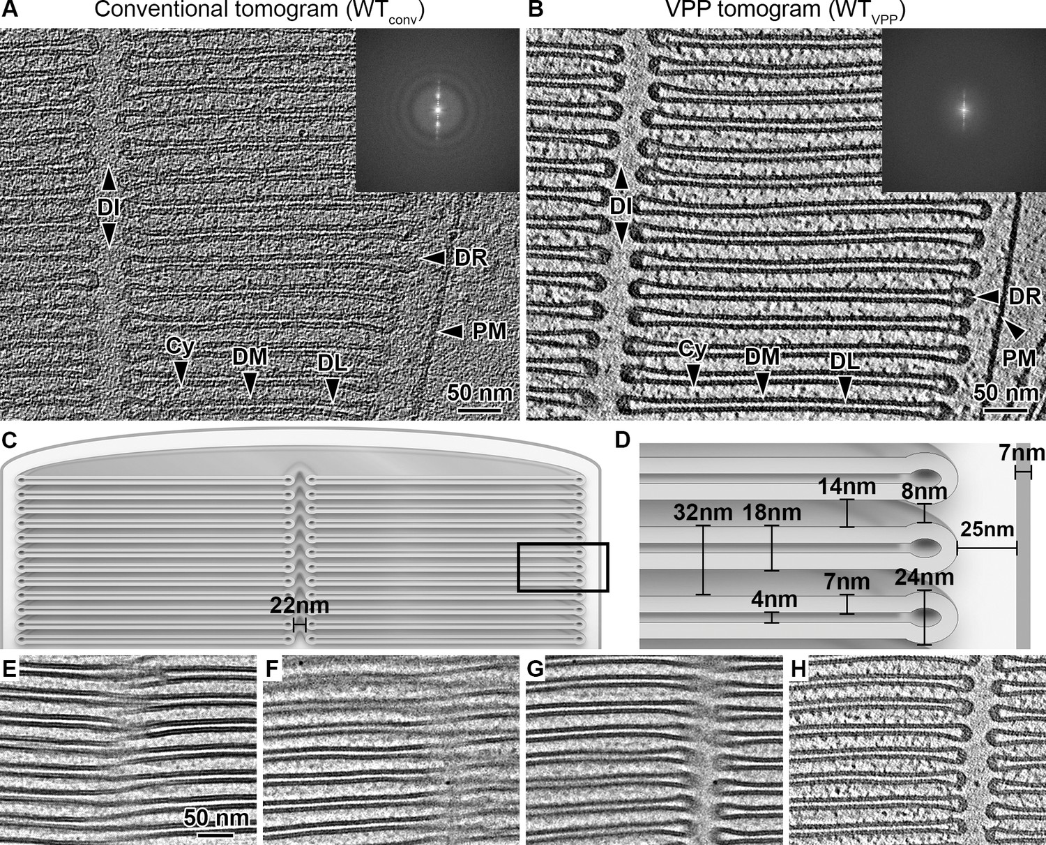
Quantitative characterization of ROS ultrastructure derived from cryo-ET.
(A) Slice through a conventional tomogram acquired at 3 μm defocus and (B) in focus with Volta phase plate (VPP). Both imaging modalities allow distinction of the ROS membranes. The disk stack is composed of disk membranes (DM) surrounded by the disk rim (DR) and interrupted by the disk incisure (DI). The disk stack is enclosed by the plasma membrane (PM). DL denotes the disk lumen and Cy the cytosol. Insets: Fourier transforms of single projection images contributing to the tomograms. (C–D) Quantification of the characteristic ROS ultrastructure. The frame in (C) indicates the field of view in (D). (E) High-dose projection (~20 e-/Å2) showing a zipper-like structure. (F) Projection from a tomographic tilt-series (~1.4 e-/Å2) at tilt angle 25° showing a zipper-like structure similar to (E). (G) Projection at tilt angle 9°. (H) Tomographic slice reconstructed from the tilt-series. Zipper-like structure in (F) is resolved into the incisure.
Figure 1—figure supplement 1
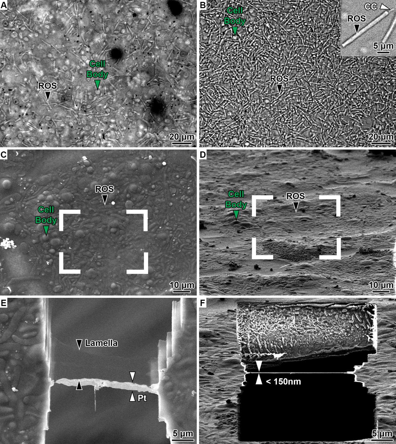
Preparation of isolated mouse rod outer segments for cryo-ET.
(A–B) Transmission light microscopy of ROS after extraction. (A) This panel shows the extract after vortexing, and (B) the supernatant after centrifugation. Black arrowheads indicate ROS, the green arrowheads indicate cell bodies. The inset in (B) shows an isolated ROS with the connecting cilium (CC) attached. (C–D) SEM and FIB images of grid square before cryo-FIB milling, respectively. ROS appear as elongated, sausage-like structures, while cell bodies appear as spherical objects. (E–F) SEM and FIB images of the area outlined in (C) and (D) after FIB milling, respectively. Pt indicates the protective layer of organo-metallic platinum.
Figure 1—figure supplement 2
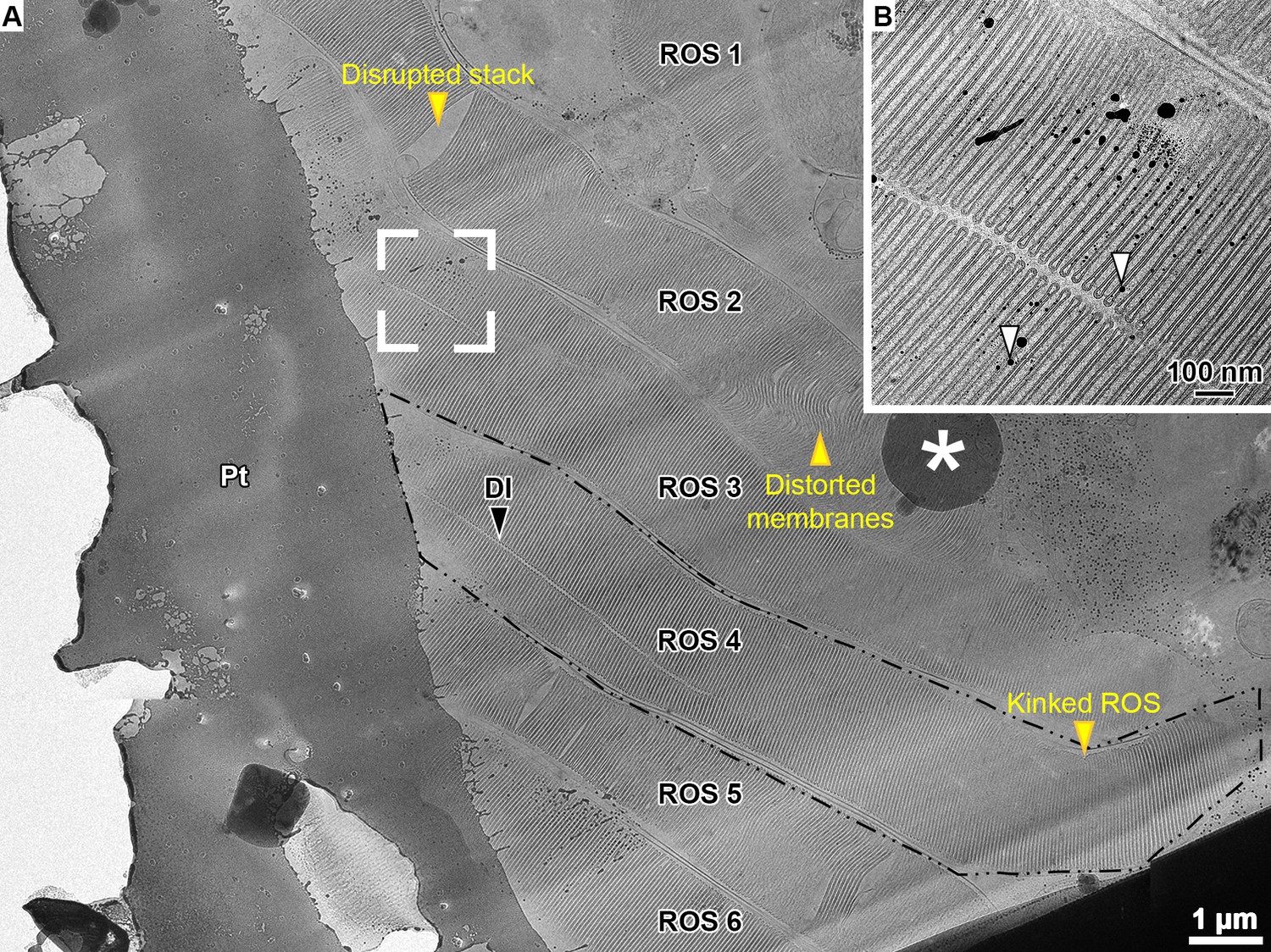
Transmission electron microscopy overview image of a lamella.
(A) Fraction of a lamella TEM overview image. It comprises six ROS oriented in parallel. One ROS is outlined in black. ROS damage is marked by yellow arrowheads. Pt denotes the protective layer of organo-metallic platinum, DI is the disk incisure and, the white asterisk indicates ice crystal contamination. Tomographic tilt-series were only acquired in areas without obvious ROS damage like the area outlined in white. (B) Projection of a tilt-series acquired in the white framed area in (A). Platinum particles which were deposited on lamellae during milling are indicated with white arrowheads and were used for tilt-series alignments.
Figure 1—figure supplement 3
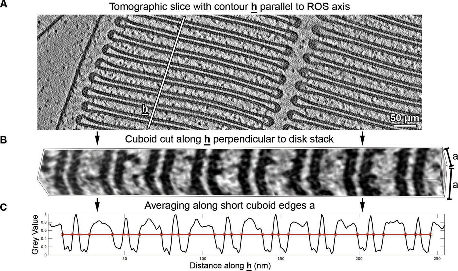
Measurement of the repetitive distances between ROS disk membranes.
(A) Contours perpendicular to the disk stack marked with (h) were defined in 4 x binned tomograms (pixel size = 10.48 Å). (B) Cuboids were cropped along (h) with length h and square base area with edge length a = 21 voxels. (C) Cuboids were averaged along the base edges to generate 1D intensity profiles of length h. Points where the membrane signal dropped to 50% of the maximum intensity are marked by red circles. The points at half maxima were used to define the distance between membranes and the membrane thicknesses.
Figure 1—figure supplement 4
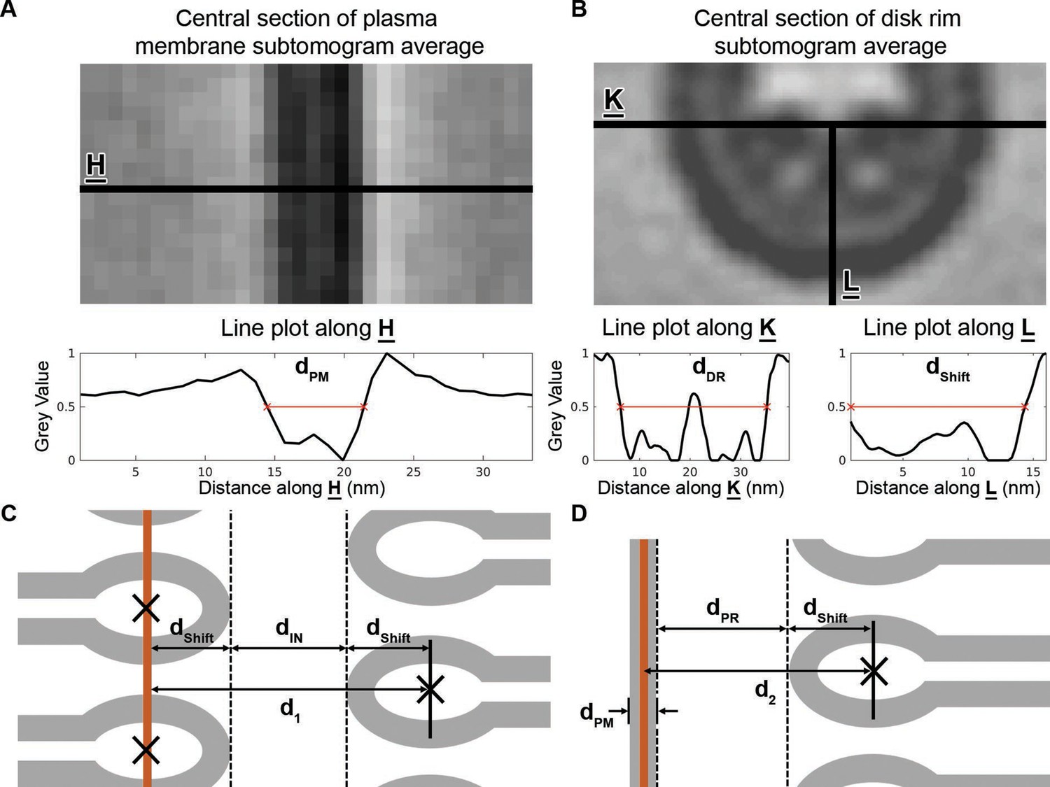
Measurements related to the plasma membrane and the disk rim.
(A–B) Thickness of the plasma membrane and measurement of the disk rim, respectively. The upper panels depict subvolume averages and define the directions (H)(K) and (L). The lower panels show intensity profiles along these directions. Characteristic distances are indicated as red lines. (C) Measurement of the cytosolic gap at the disk incisure dIN. (D) Measurement of the cytosolic gap between the disk rim and the plasma membrane dPR. The orange line represents the central plane of the PM as estimated by segmentation.
Figure 1—figure supplement 5
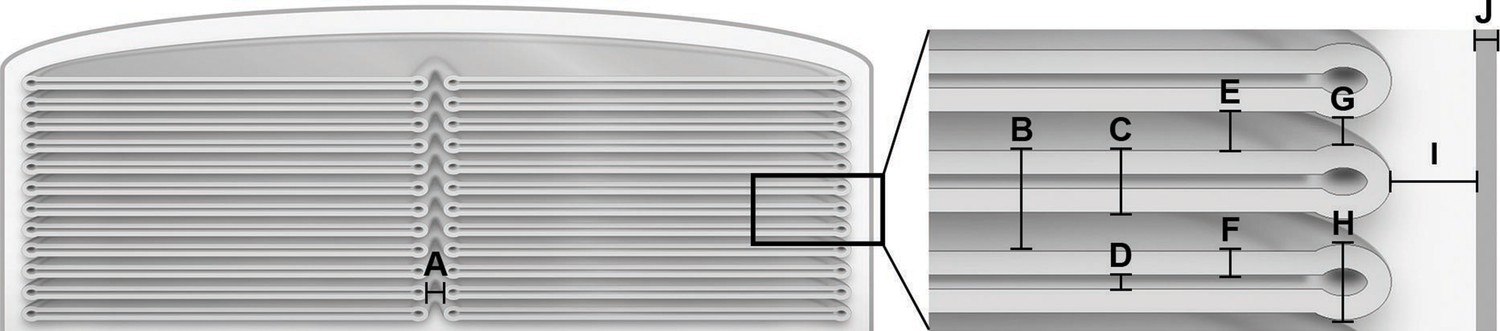
Mean values and standard deviations (SD) of the measured ROS distances.
The letters in the table are assigned to distances in the sketch in the upper panel.
Figure 2 with 4 supplements
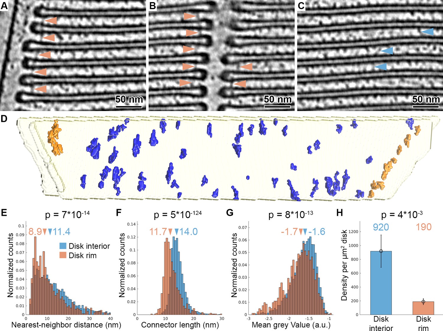
Tomography with VPP reveals molecular connectors between membranes of adjacent disks.
(A–C) Slices of a tomogram acquired in focus with VPP (WTVPP), filtered with a Gaussian Kernel (sigma = 4 voxel). Orange arrowheads in (A) and (B) indicate connectors localized at the disk rim in proximity to the plasma membrane and the disk incisure, respectively. Blue arrowheads in (C) point at connectors between the parallel membranes of adjacent disks in the disk interior. (D) Connectors segmented with the customized Pyto workflow on the example of one membrane pair viewed from the top (along ROS axis). Connectors within 40 nm of the outer disk periphery are defined as disk rim connectors (orange), and connectors in between the parallel membrane planes as disk interior connectors (blue). (E–G) Statistical analysis of 7000 connectors from five tomograms of the WTVPP dataset. Histograms are shown of nearest neighbor distances (E), connector length (F) and mean gray value (G). Arrowheads above the histograms indicate the median values. (H) Mean value of connector density per µm2 of total disk membrane determined in five tomograms (error bars: one standard deviation). p Values were calculated according to the two-sample Kolmogorov-Smirnov test.
Figure 2—figure supplement 1
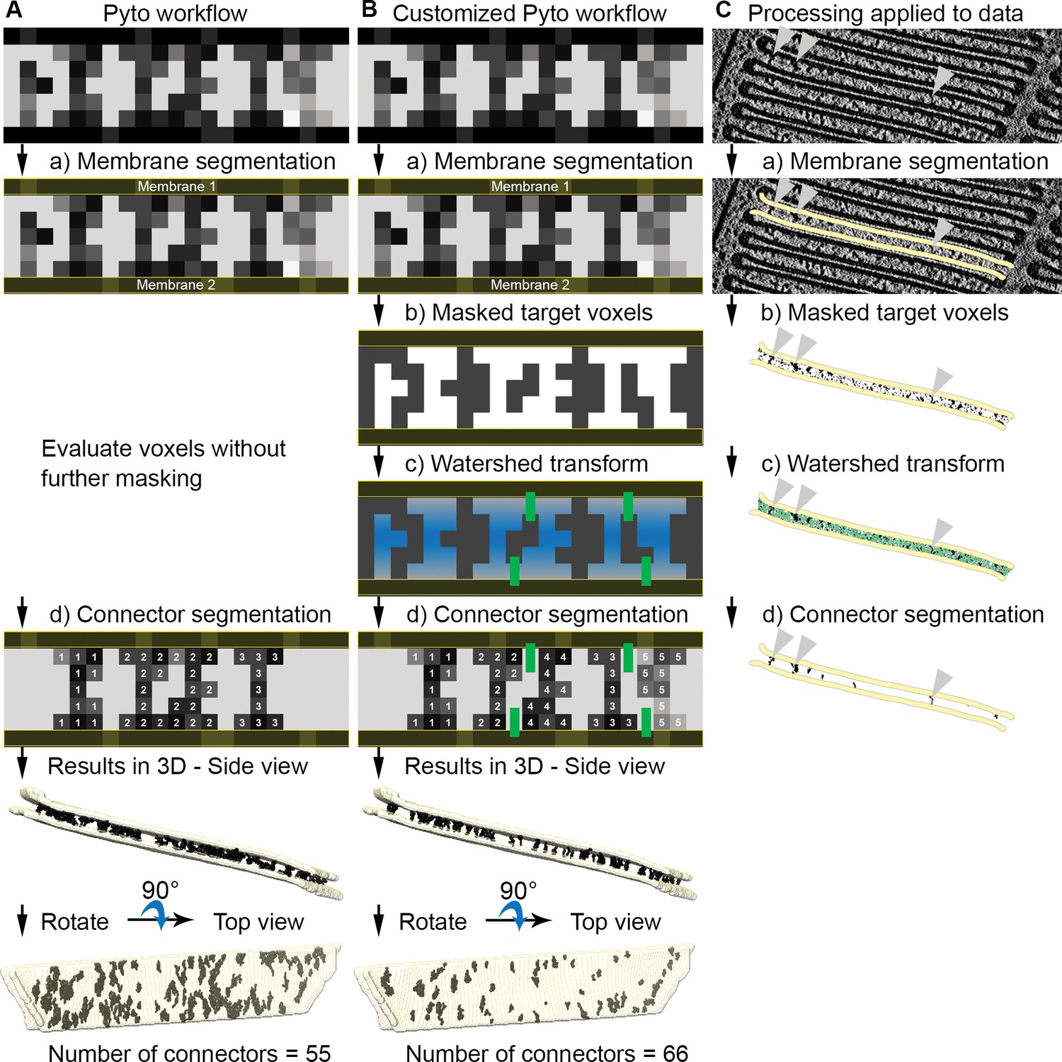
Connector segmentation with the customized Pyto workflow.
(A) The original Pyto workflow. (B) The customized Pyto workflow involving the creation of a binary mask with a single threshold. The binary mask is then subjected to watershed transform with ‘catchment basins’ filled from the center between the membranes towards the outside as indicated by the gradient of blue color in step (c). Watershed lines are shown as green bars. (C) The customized Pyto workflow applied to actual data on the example of one membrane pair. Membrane masks are depicted in yellow, watershed lines in green and segmented connectors in black. Connectors that can be tracked throughout the processing pipeline are marked by gray arrowheads.
Figure 2—figure supplement 2
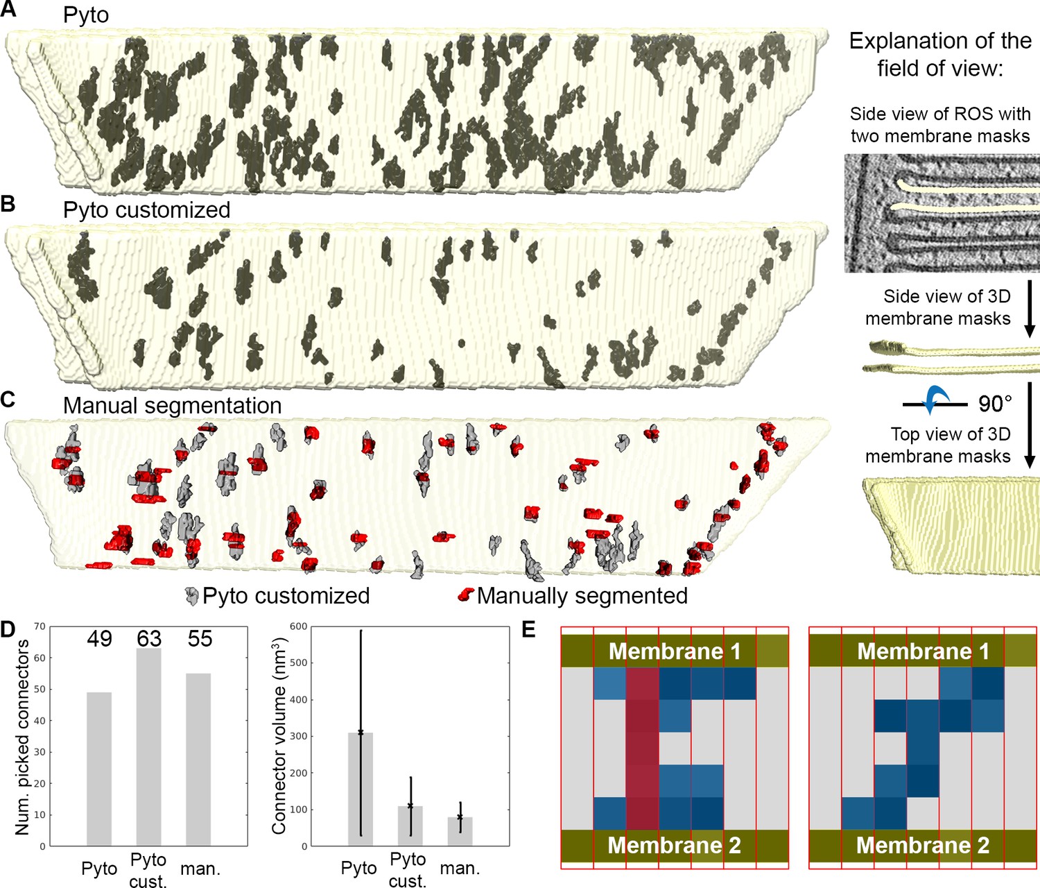
Comparison of segmentation methods for one membrane pair viewed from the top.
(A) Segmentation results of the original Pyto workflow. The neighboring membranes of adjacent disks are depicted in yellow. The segmented connectors are black. (B) Results with the customized Pyto workflow. (C) Comparison of results in B with manual segmentation. The right panel explains the viewing direction in (A–C). (D) Number of picked connectors and average connector volume for the segmentation methods (error bars: one standard deviation). (E) Sketch of connectors to illustrate the reason for differences between manual and automated segmentation. The membrane pair is viewed from the side (perpendicular to the ROS axis). Red rectangles represent tomographic slices. Manually and automatically segmented voxels are filled red and blue, respectively. The membranes are yellow. The Left panel indicates why manually selected connectors have a smaller volume. The right panel illustrates an inclined connector. In none of the slices is it observed as a straight connector. Therefore, it can be missed in the manual segmentation.
Figure 2—figure supplement 3
Considerations for the statistical analysis and classification of connectors.
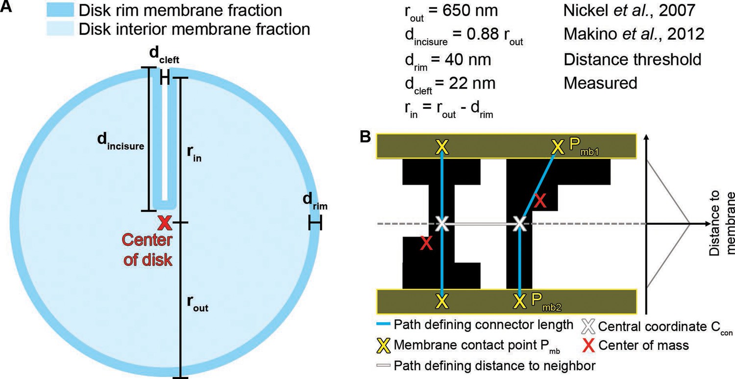
(A) Disk morphological considerations to calculate the rim, interior, and total membrane area. (B) Sketch of two connectors illustrating the characteristic connector points. For each connector, the membrane contact points Pmb and the central point Ccon were used to calculate the connector length. Ccon of neighboring connectors was used to compute the nearest-neighbor distances.
Figure 2—figure supplement 4
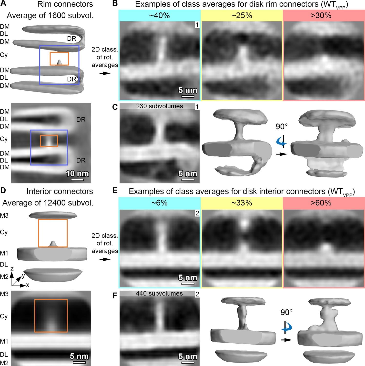
Classification and averaging of disk connectors.
(A) Initial alignment of all disk rim connectors. The isosurface representation of the average is shown in the upper panel, the cross-section through the center in the lower panel. DM denotes disk membranes, DL the disk lumen, Cy the cytosol and DR the disk rim. The orange box marks the outline of the mask used for classification, the blue box the field of view in (B) and (C). (B) Three examples for class averages. A promising class which appears as a straight connector is boxed in green, an ambiguous class in yellow and a false-positives class in red. (C) Subvolume alignment of the promising class labelled with ‘1’ in (B). The left panel shows a cross section through the center of the average, middle and right panels are isosurface representations from two orientations. They display a clear connector between neighboring disk rims, but no further structural information can be inferred. (D–F) Similar analysis for disk interior connectors. (D) shows the initial alignment of all connectors, (E) three examples for class averages and (F) the alignment of the promising class labelled with ‘2’ in (E). M1 indicates the membrane at which the subvolume was extracted, M2 the second membrane within the same disk and M3 the neighboring disk.
Figure 3 with 5 supplements
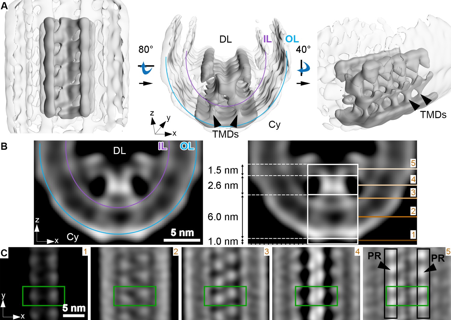
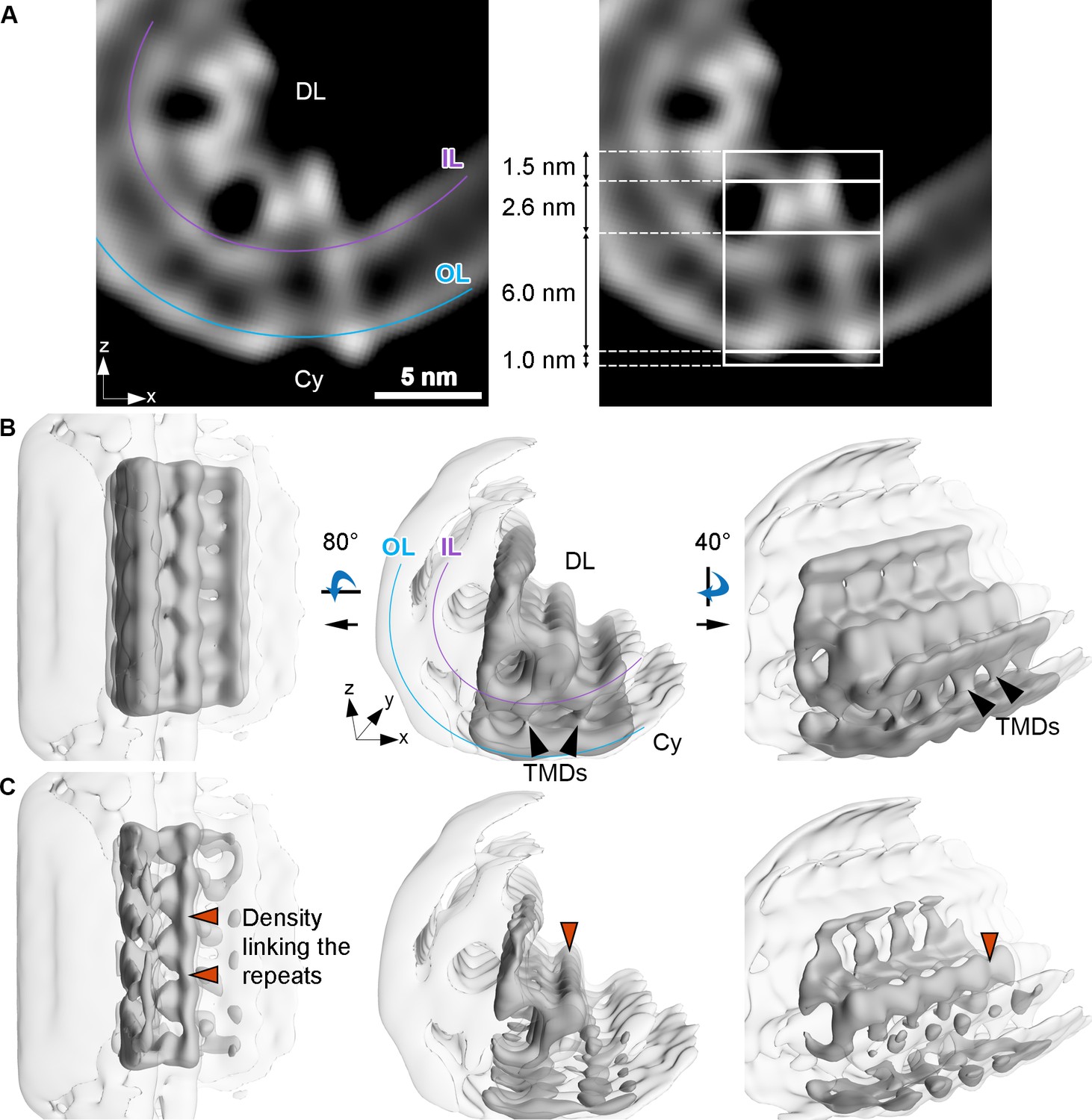
Membrane curvature at the disk rim is organized by a scaffold composed of three rows.
This average was obtained by focusing the alignment on four repeats along the central density row (CD). (A) Isosurface representation of the disk rim subvolume average. The central row of density with its contacts to the peripheral rows is depicted in solid gray by applying the alignment mask to the average, and the signal of the whole disk rim average is shown in transparent grey. Black arrowheads indicate transmembrane densities (TMDs). DL denotes the disk lumen and Cy the cytosol. (B) Cross-sections through the disk rim average density without masking. (C) Orthogonal slices of the unmasked averageat different z-heights. The green box is centered on the same repeat along the central density row throughout the slices. In the right panel, the signals of the peripheral rows (PR) are marked by black boxes. The locations of the slices are indicated by numbered lines in the right panel of (B). The signal of the inner leaflet (IL) and outer leaflet (OL) are indicated by a purple and a blue line, respectively.
Figure 3—figure supplement 1
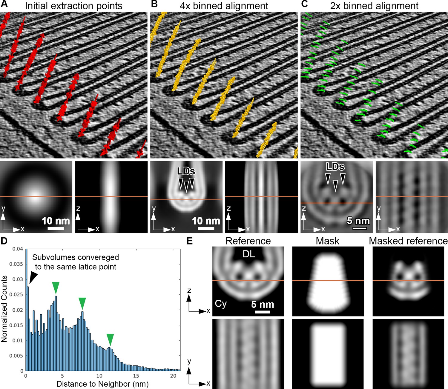
Picking and alignment of disk rim subvolumes.
(A–C) Positions and orientations of subvolumes with the corresponding averages for different alignment steps. In the top panel, each arrow represents the position of one subvolume and the arrow direction coincides with the subvolume z-axis. The bottom panel depicts two orthogonal sections through the corresponding subvolume average. The location of the slices through the average are indicated by orange lines. The initial extraction points are shown in (A), the refined positions after alignment of 4 x binned subvolumes in (B) and the distance-cleaned positions after alignment of 2 x binned subvolumes in (C). Luminal densities (LDs) are indicated by black arrowheads. (D) Histogram of distance to 10 nearest neighbors for positions of 2 x binned particles before distance cleaning. Green arrowheads indicate peaks at multiples of 4 nm for subvolumes partially converged into lattice points. (E) Reference and mask used for the alignment of unbinned subvolumes. The initial reference, the mask and the masked reference are shown in the left, middle, and right panels, respectively. The orange line in the upper panel indicates the position of the slice in the lower panel. DL denotes the disk lumen and Cy the cytosol.
Figure 3—figure supplement 2
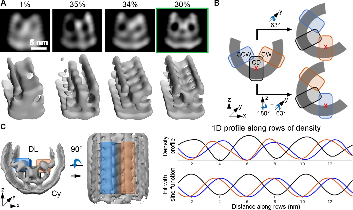
Classification and analysis of the disk rim scaffold.
(A) Examples for class averages obtained for the central row of density by classification of disk rim subvolumes in RELION (Scheres, 2016) indicating the local flexibility of the disk rims. The upper panel shows a slice through the center of the average, the lower panel shows the isosurface representation. The class highlighted in the green frame was used for further processing. (B) Sketch to illustrate the symmetry operations used to align the clockwise- (CW) and counterclockwise (CCW) rows of density with respect to each other. The starting points were the orientations of the central density (CD) row. The subvolume extraction points are marked by red crosses. (C) Intensity profiles along the three rows. Gray values were extracted from the whole, unmasked WTconv average of the central density row (CD). The left panel indicates the orientation of the three masks used to calculate the 1D intensity profiles in the right panel. The top right panel shows the actual 1D signals and the middle right panel the fitted sine-functions. The parameters of the fit are listed in the bottom panel. DL denotes the disk lumen and Cy the cytosol.
Figure 3—figure supplement 3
Subvolume average of the peripheral rows in the disk rim.
This average was obtained by focusing the alignment on four repeats along the peripheral rows (PR). (A) Cross-section through the PR average without masking. The shape of the repeats in the peripheral rows is overall similar to the repeats of the central row (Figure 3B) but exhibit slight distortion or inclination towards the central repeat. (B) Isosurface representations of the PR average from different perspectives. The peripheral row and its contact to the neighboring row is shown in solid gray by applying the alignment mask to the average, and the signal of the whole, unmasked PR average in transparent gray. Black arrowheads indicate transmembrane densities (TMDs). (C) Same perspectives as in (B) but with isosurface representations at higher threshold. The density which links repeats of the peripheral row is highlighted by orange arrowheads. DL denotes the disk lumen and Cy the cytosol. The signals of the inner leaflet (IL) and outer leaflet (OL) are indicated by a purple- and a blue line, respectively.
Figure 3—figure supplement 4
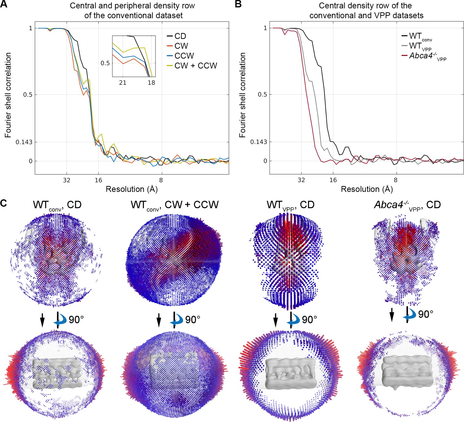
Fourier shell correlation and angular distribution of disk rim averages.
(A) Fourier shell correlation (FSC) curves for the subvolume averages derived from the conventional dataset (WTconv). (CD) denotes the central-, CW the clockwise-, CCW the counterclockwise rows, and CW + CCW combined both peripheral rows. (B) FSC curves for averages of the central density row. WTconv and WTVPP denote the conventional and the VPP dataset of WT mice, respectively. Abca4-/-VPP is the VPP dataset of ABCA4 knockout mice. (C) Angular distribution of the subvolume averages.
Figure 3—figure supplement 5
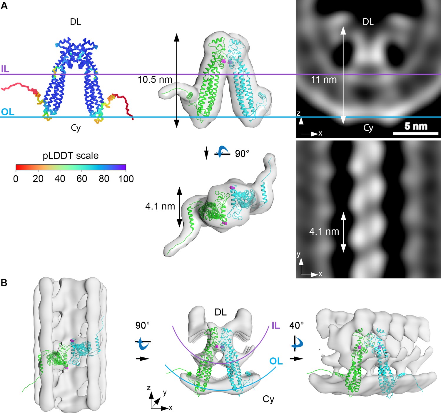
Prediction of the PRPH2 dimer with ColabFold.
(A) Comparison of the PRPH2 dimer model with the repeat resolved in the disk rim subvolume average. The left panel shows a front view of the model predicted by ColabFold colored according to the predicted local distance difference test (pLDDT). The middle panel depicts front and top view of the same model and a density map filtered to a resolution of 18 Å. The first and the second PRPH2 chain of the dimer are colored in green and cyan, respectively. The PRPH2-C150 cysteine residues responsible for intermolecular disulfide bonds are indicated by magenta spheres. The right panel shows slices through the whole, unmasked disk rim subvolume average. (B) The predicted model of the PRPH2 dimer docked into one repeat along the central density row of the disk rim scaffold. PRPH2-C150 is colored magenta, the two PRPH2 chains in green and cyan. The central row of repeats and its contact to the peripheral rows as isosurface representation is shown in transparent gray by applying the alignment mask to the whole disk rim average. DL denotes the disk lumen and Cy the cytosol. The signals of the inner leaflet (IL) and outer leaflet (OL) are indicated by a purple- and a blue line, respectively.
Figure 4
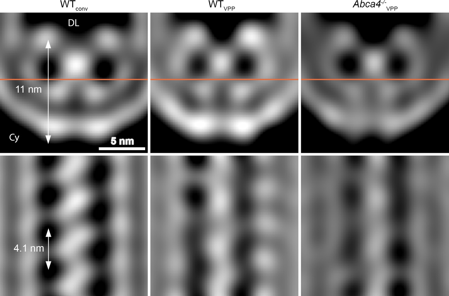
Comparison of the disk rim scaffold in WT and abca4-/- mice.
Shown are orthogonal slices through the whole, unmasked averages of the central density (CD) in different datasets. All averages are filtered to a resolution of 30 Å. The left and right panel display the average of WT disk rims from a conventional (WTconv) and a VPP dataset (WTVPP). The right panel shows the VPP average derived from ABCA4 knockout mice (Abca4-/-vpp). The orange line in the upper panels indicates the location of the slice in the bottom panels. DL denotes the disk lumen and Cy the cytosol.
Figure 5
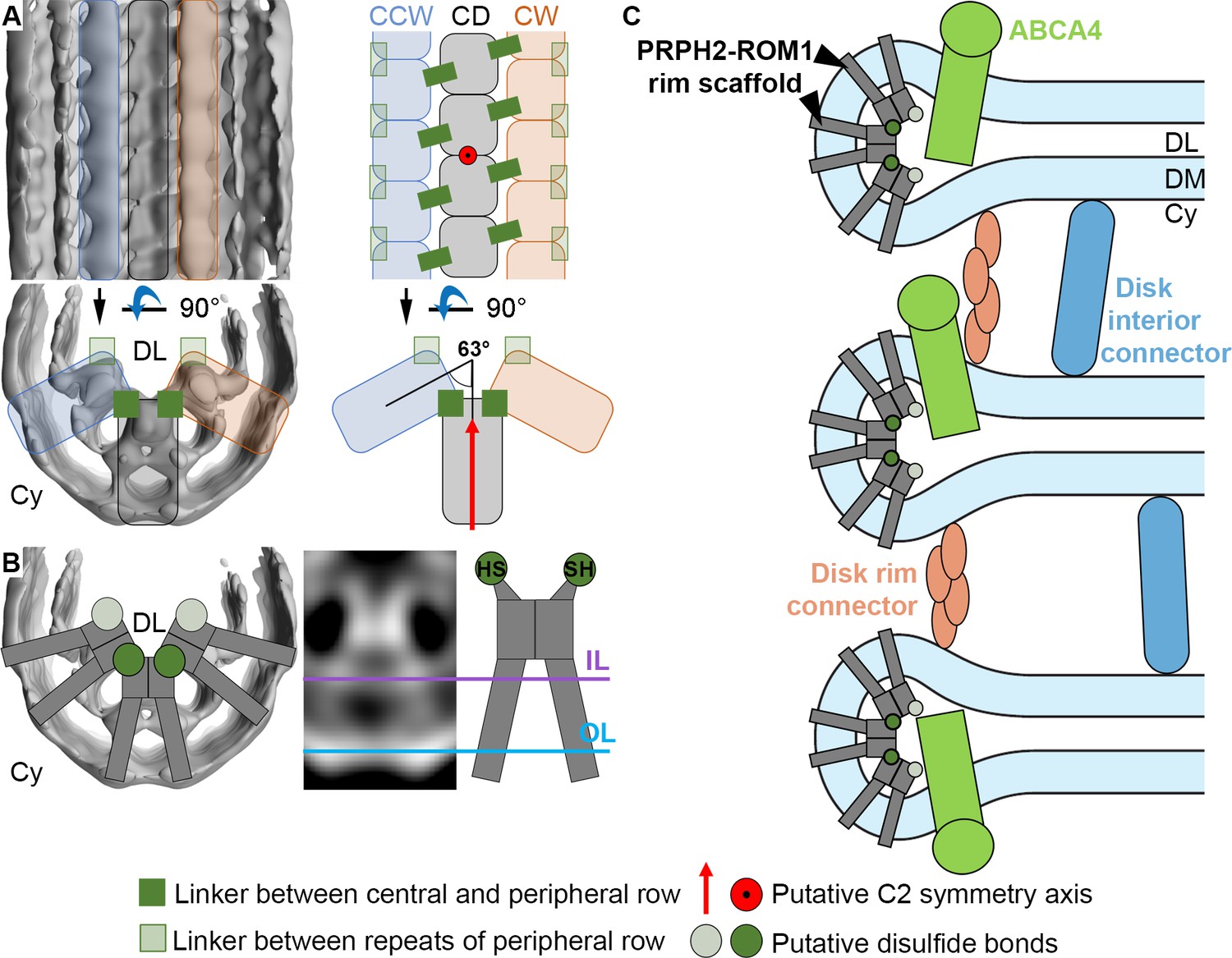
Models for the organization of ROS disk rims and the disk stack.
(A) The general organization of the disk rim scaffold. (CD) marks the central density row, CW and CCW the clockwise- and counterclockwise peripheral row. (B) Non-covalently bound, V-shaped PRPH2-ROM1 complexes assemble into the disulfide bond-stabilized disk rim scaffold. We hypothesize that the PRPH2-C150 and ROM1-C153 cysteine residues which are responsible for intermolecular disulfide bonds are located in the head domain of the complexes forming the contacts between rows and repeats of the peripheral rows. (C) An updated model for the organization of the ROS disk stack. DL denotes the disk lumen, Cy the cytosol, and DM the disk membranes.
Videos
Video 1
Slices through a conventional tomographic volume acquired without Phase Plate and 3 µm defocus.
Scale bar 50 nm.
Video 2
Tilt series of a tomogram acquired in focus with Volta Phase Plate.
Scale bar 50 nm.
Video 3
Slices through the tomographic volume after weighted back projection of the tilt series in Video 2.
In focus with Volta Phase Plate. Scale bar 50 nm.
Video 4
Slices through a tomographic volume filtered with a Gaussian Kernel (sigma = 4 voxel).
Shown are ROS disk rims in proximity to the plasma membrane. Many straight connectors between the disks can be observed at the disk periphery. Scale bar 20 nm.
Video 5
Slices through a tomographic volume filtered with a Gaussian Kernel (sigma = 4 voxel).
Shown are the parallel ROS disk membranes (disk interior). Structures that interconnect the disks can be found but are less abundant than at the disk periphery (Video 4). Scale bar 20 nm.
Video 6
Segmentation of connectors between two adjacent disks.
Color code: yellow: membrane mask; blue: connectors in the disk interior; orange: connectors at the disk rim.
Video 7
Orientation of the disk rim subvolume average with respect to disk rims in the tomograms.
The top panel shows a tomographic slice (WTVPP) with one disk rim indicated by an orange frame. The bottom panel depicts the isosurface representation of the disk rim average obtained by focusing the alignment on the central density row. The view along the disk periphery reveals three luminal densities which form a continuous scaffold of three interconnected rows along the disk rim.
Video 8
Isosurface representation of the disk rim subvolume average.
This average was obtained by focusing the alignment on four repeats along the central row of density. Initially, the whole, unmasked average is shown. Later, the central row of density (CD) with its contact to the peripheral rows (PR) is shown in solid grey by applying the alignment mask while the signal of the whole disk rim is displayed in transparent gray. The same representation was used in Figure 3A.
Video 9
Isosurface representation of the disk rim subvolume average for the peripheral rows (CW+ CCW).
This average was obtained by centering the peripheral row (PR) in the subvolume box and focusing the alignment on four repeats along the PR. Initially, the whole, unmasked average is shown. Later, the peripheral row (PR) with its contact to the central density rows (CD) is shown in solid gray by applying the alignment mask while the signal of the whole disk rim is displayed in transparent gray. The same representation was used in Figure 3—figure supplement 3B.
Video 10
Isosurface representation of the disk rim subvolume average for the peripheral rows (PR).
This is the same average as in Video 9 with a similar representation, but at higher threshold emphasizing the density which links the repeats within the PR on the outside of the disk rim scaffold.
Video 11
Predicted model of a PRPH2 dimer docked into a repeat along the central row of density.
The central row of density with its contact to the peripheral rows is shown in transparent grey by applying the alignment mask the whole disk rim average. The two PRPH2 chains within the dimer model are colored in green and cyan. The PRPH2-C150 cysteines are indicated as spheres in magenta.
Tables
Table 1
List of used datasets.
| Dataset abbreviation | WTconv | WTVPP | Abca4-/-VPP | |
|---|---|---|---|---|
| Mouse sample | Wild type | Wild type | Abca4-/- | |
| Volta phase plate | No | Yes | Yes | |
| Defocus (µm) | 3 | 4.5 | 0 | 0 |
| # Tomograms | 36 | 12 | 18 | 6 |
| EMPIAR accession code (EMPIAR-) | 10773 | 10772 | 10771 | |
| Number of segmented connectors in five tomograms | ||||
| Disk rim connectors | - | 800 | - | |
| Disk interior connectors | - | 6,200 | - | |
| Disk rim subvolumes for central density (CD) | ||||
| # all subvolumes | 53,000 | 14,300 | 4,600 | |
| # classified subvolumes | 9,000 | 11,000 | 3,400 | |
| Global resolution at FSC = 0.5 (Å) | 18.6 | 22.5 | 27.5 | |
| Global resolution at FSC = 0.143 (Å) | 16.9 | 19.9 | 22.7 | |
| Processing with Warp/M | Yes / Yes | No / No | No / No | |
| EMDB accession code (EMD-) | 13321 | 13323 | 13324 | |
| Disk rim subvolumes for peripheral density (CW+ CCW) | ||||
| # all subvolumes | 106,000 | - | - | |
| # classified subvolumes | 48,000 | - | - | |
| Global resolution at FSC = 0.5 (Å) | 18.2 | |||
| Global resolution at FSC = 0.143 (Å) | 16.8 | - | - | |
| Processing with Warp/M | Yes / Yes | |||
| EMDB accession code (EMD-) | 13322 | |||
Additional files
Download links
A two-part list of links to download the article, or parts of the article, in various formats.
Downloads (link to download the article as PDF)
Open citations (links to open the citations from this article in various online reference manager services)
Cite this article (links to download the citations from this article in formats compatible with various reference manager tools)
Determinants shaping the nanoscale architecture of the mouse rod outer segment
eLife 10:e72817.
https://doi.org/10.7554/eLife.72817


