Parent-of-origin effects propagate through networks to shape metabolic traits
Figures
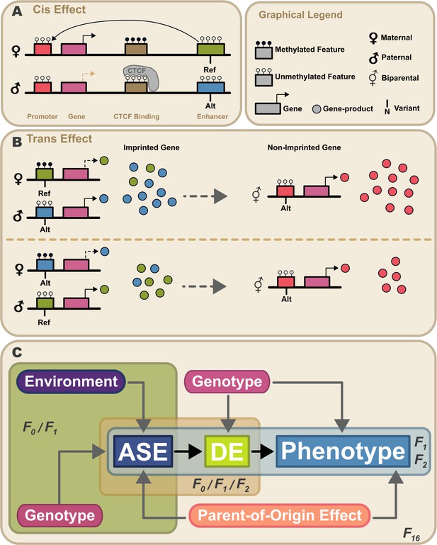
Proposed model for propagation of parent-of-origin effects through gene-gene interactions.
Parent-of-origin effects should be partitioned into cis mechanisms and trans mechanisms (A) An example of a cis parent-of-origin effect is a system with three regulatory elements: promoter, insulator, and enhancer. Activation of transcription requires the enhancer to act upon the promoter. Enhancer activity is blocked by the insulator when it has been bound by CTCF. CTCF cannot be bound when methylated. In this system, the insulator is selectively methylated when inherited maternally, so methylation of the maternally inherited insulator blocks CTCF binding, allowing the enhancer to activate transcription. Because the paternally inherited insulator is not methylated, it is bound by CTCF which blocks enhancer activity, silencing transcription. This canonical genomic imprinting mechanism interacts with genetic variation in the three regulatory features. For example, if one allele produces stronger enhancer activity (Alt) than the other, individuals inheriting the Alt allele maternally would have elevated expression compared to those that inherit the same allele paternally. These cis genetic effects do not occur in isolation. Due to the highly interconnected nature of biological systems, there are downstream effects. We refer to these as trans parent-of-origin effects. (B) An example of a trans parent-of-origin effect is a system with two genes each having its own promoter. The first gene is canonically imprinted, and the activity of the gene promoter is blocked by DNA methylation. The imprinted gene’s promoter is methylated when inherited maternally. Consequently, the paternally inherited allele is almost exclusively expressed. As before, when genetic variation in a regulatory feature interacts with these epigenetic mechanisms, we see parent-of-origin effects on expression of the imprinted gene. In this example, the imprinted gene regulates expression of a non-imprinted gene. Despite the non-imprinted gene being agnostic to parental origin, its expression nonetheless depends on the parental origin of alleles at the imprinted locus. (C) Summary of our experimental design. Expression patterns of genes showing allele-specific expression (ASE) such as imprinted genes are shaped by parental genotypes and environment (e.g. nutrition). Downstream gene expression is a function of their genotype and the expression of upstream ASE genes. Altered parent-of-origin dependent total gene expression of ASE genes leads to differential expression of downstream genes varying only in allelic parent-of-origin (DE). Phenotype is most directly affected by expression of DE genes. Variation in DE gene expression leads to corresponding variation in phenotype. Mouse populations used to probe parts of this model are labeled F0 (inbred lines), F1 (reciprocal cross of inbred lines), F2 (intercross of F1 mice), and F16 (advanced intercross of inbred lines).
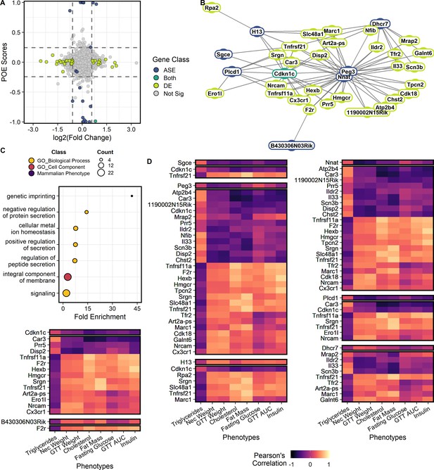
Genes showing parent-of-origin effects at the allele specific and/or total expression levels covary with each other and with metabolic traits.
(A) Mean parent-of-origin effect score across contexts. Effect size of ASE is calculated as the mean allelic bias (L / L + S) of SxL animals minus LxS animals. Effect size of DE is measured by log2(Fold Change) between LxS and SxL crosses. The single context with largest magnitude fold change is plotted for each gene. Dashed lines represent minimum acceptable effect size cut-offs within a context. Genes showing significant ASE and sufficiently large parent-of-origin effect score are shown in blue. Genes showing significant DE and sufficiently large fold change in some sex or dietary context are shown in lime. Genes showing both ASE and DE are shown in teal. Genes not meeting cut-offs are shown in gray. The two genes showing significant ASE but falling short of parent-of-origin effect score requirements are a case of context dependent bipolar parent-of-origin effect scores (i.e. paternally expressed in one context and maternally expressed in its opposite). (B) Parent-of-origin effect network constructed from ASE and DE gene pairs. (C) Significantly overrepresented ontologies after multiple tests correction in the parent-of-origin effect network. Terms are color coded by ontology domain. GO biological process (yellow), GO cellular component (orange), and Mammalian phenotype (purple). Circle size denotes the number of genes with each term. (D) Correlation of parent-of-origin effect network genes with metabolic traits. Only genes and phenotypes with at least one significant correlation after multiple test corrections are shown. The heatmap is broken up into subnetworks with the ASE gene as the first separated row followed by associated DE genes in subsequent rows. Columns correspond to metabolic traits. Coloration of each cell denotes the Pearson’s correlation coefficient value.
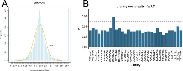
RNAseq libraries are sufficiently complex to detect allele specific expression.
Complexity was measured by fitting a beta-binomial distribution to the distribution of Lbias values. A representativeIn this study, we use four populations at distribution (A) of Lbias values (blue) and fit beta-binomial (orange). The shape parameters (α, β) of the beta-binomial distribution are used to calculate dispersion (ρ). Dispersion value less than 0.05 indicate sufficient complexity. One library was not sufficiently complex (B) and was removed from analyses.
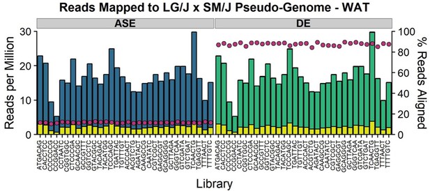
Number of reads mapped to LG/J x SM/J pseudo-genome.
We isolated total RNA from white adipose (n = 32 per sex/diet/cross cohort) and constructed RNA-Seq libraries. Libraries were sequenced 1 sample per lane on an Illumina HiSeq 4000 (Illumina, San Diego, USA) using 2 × 100 bp PE reads. FASTQ files were filtered to remove low-quality reads. Remaining reads were aligned against both LG/J and SM/J pseudo-genomes simultaneously using STAR with either multimapping disallowed (allele-specific expression, ASE) or multimapping allowed (differential expression, DE). The stacked bars denotes the number of reads per million (left y-axis) and are color-coded by category (uniquely = yellow, multi-loci = green, too many = blue). For the ASE alignment, ‘too many’ reads are defined as n > 1 since multimapping was disallowed. For the DE alignment, ‘multi-loci’ reads are defined as 1 < n < 10 and ‘too many’ reads are defined as n > 10. The pink dots denote the primary alignment rates (right y-axis) for each library. Alignment rates are defined as (# reads mapped uniquely + # reads mapped multi-loci / total # input reads).
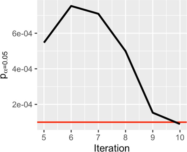
Stable null permutation plots for allele-specific expression.
Context was permuted to generate an appropriate null model of p-values. Each iteration represents one genome wide permutation where every gene (7,869) was permuted separately, thus each iteration represents 7,869 separate shuffles. Null distribution stability was evaluated by calculating the critical value (in this case a significance estimate) for alpha = 0.05 at each iteration. The standard deviation of critical values was calculated after each iteration for the last 5 iterations. The model was considered stable once variation in critical values dropped below 1e-4 (red line). The variation in critical values of the null model approaches zero over ten genome wide iterations. This approximation towards zero demonstrates the stabilization of the null model. By 10 genome wide shuffles the critical value fluctuates <1e-4 units per iteration in the most complex model, meaning that at false discovery rate estimates might vary by ±1e-4.
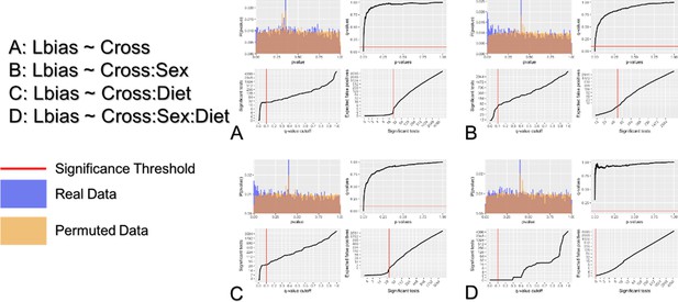
Multiple tests correction of ASE detection.
Multiple tests correction was performed by estimating the false discovery rate using a permuted null model of p-values. Context was permuted to generate an appropriate null model of p-values. The distribution of permuted (orange) and real (blue) p-values is shown for each term in the model in the top left of each subplot. False discovery rate was estimated as the proportion of tests below a given significant threshold under the null relative to the real data (Null/Real). A ratio of 1 meaning that ~100% of observations at that significance threshold are likely false discoveries. The relationship between false discovery rate and p-value threshold is shown in the top right subplot for each mode. The number of significant tests at a given acceptable false discovery rate is shown as the bottom left subplot for each model. The number of false positives relative to the number of significant tests is shown as the bottom right subplot for each model.

Volcano plots of parent-of-origin dependent allele-specific expression.
Log10 transformed FDR plotted against POE score [ mean SxL Lbias – mean LxS Lbias ] for each context. Genes passing both POE score and significance thresholds are shown in orange. Genes failing to meet these criteria are shown in gray.
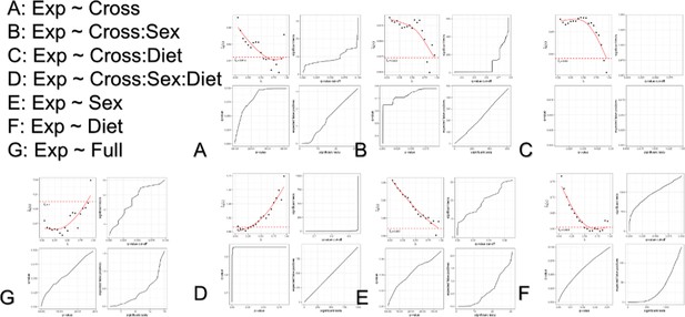
Multiple tests correction of DE detection.
Multiple tests correction was performed by estimating the false discovery rate using the ‘qvalue’ R package without the generation of a permuted null model. The underlying null model is selected by the model by controlling . False discovery rate (q-value) is estimated as the proportion of tests below a given significant threshold derived from the estimated null model relative to the real model (Null/Real). A ratio of 1 meaning that ~100% of observations at that significance threshold are likely false discoveries. The selection of is shown in the top left of each subplot for each model. The relationship between false discovery rate and p-value threshold is shown in the bottom left subplot for each mode. The number of significant tests at a given acceptable false discovery rate is shown as the top right subplot for each model. The number of false positives relative to the number of significant tests is shown as the bottom right subplot for each model.
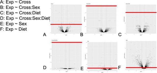
Volcano plots of differentially expressed genes.
Log10 transformed FDR plotted against log2 transformed fold change for each context. The FDR threshold we used was 0.1 (red line).
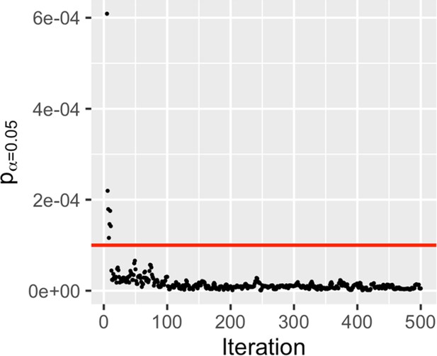
Stable null permutation plots for network pairs.
Context and expression were permuted to generate an appropriate null distribution of p-values. Significance for each pair was estimate by likelihood ratio test using a chi-squared approximation. Null distribution stability was evaluated by calculating the critical value (in this case a significance estimate) for alpha = 0.05 at each iteration. The standard deviation of critical values was calculated after each iteration for the last 5 iterations. The model was considered stable once variation in critical values dropped below 1e-4 (red line). The variation in critical values under the null model approaches zero over 100 iterations. By 500 shuffles the critical value fluctuates well below 1e-4 units per iteration in the most complex model, meaning that at worst FDR estimates would vary by well below ±1e-4.
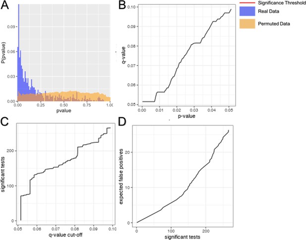
Multiple tests correction of pairwise network construction.
Multiple tests correction was performed by estimating the false discovery rate using a permuted null model of p-values. The distribution of permuted (orange) and real (blue) p-values is shown (A). False discovery rate was estimated as the proportion of tests below a given significant threshold under the null relative to the real data (Null/Real). A ratio of 1 meaning that ~100% of observations at that significance threshold are likely false discoveries. The relationship between false discovery rate and p-value threshold is shown (B). The number of significant tests at a given acceptable false discovery rate is shown (C). The number of false positives relative to the number of significant tests is shown (D).
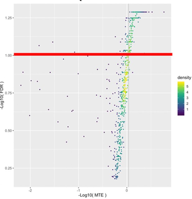
Volcano plots of network construction.
Log10 transformed FDR is plotted against log10 transformed mean test error (MTE). The FDR threshold value of 0.1 is shown as the red line. The MTE threshold was set to the upper 1th percentile of the permuted model MTE and is show as the gray vertical line. Each gene is represented by a single point. Coloration of points is determined by the joint FDR/MTE density.
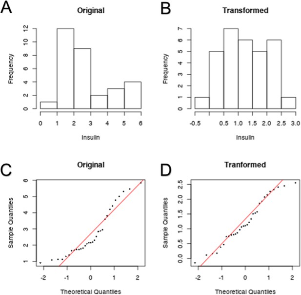
Example transformation of F1 phenotypes.
In order to meet the assumptions of normality required by Pearson’s correlation test, non-normally distributed phenotypes were log transformed. Normality was evaluated by Shapiro-Wilkes test (p < 0.05 indicates non-normality). Serum insulin is one such phenotype. The probability distribution of serum insulin is shown before (A) and after transformation (B). This distribution is also compared to a normal distribution via quantile-quantile plot before (C) and after (D) transformation.
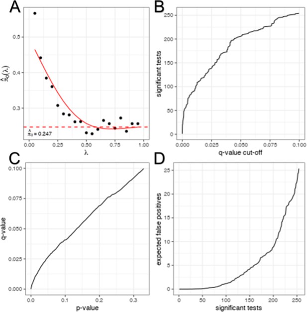
Multiple tests correction of phenotype correlations.
Multiple tests correction was performed by estimating the false discovery rate using the ‘qvalue’ R package without generating a permuted null model. The underlying null model is selected by controlling . False discovery rate (q-value) is estimated as the proportion of tests below a given significant threshold derived from the estimated null model relative to the real model (Null/Real). A ratio of 1 meaning that ~100% of observations at that significance threshold are likely false discoveries. Selecting (A) allows us to determine the relationship between false discovery rate and p-value threshold (C). Using this relationship, we can determine the number of significant tests at a given acceptable false discovery rate (B). From this we can determine the number of false positives relative to the number of significant tests (D).
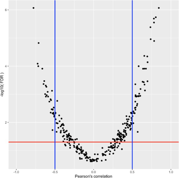
Volcano plots of phenotypes correlated with POE net gene expression.
Log10 transformed FDR plotted against Pearson’s correlation coefficient. Each dot represents a phenotype/gene pair. The FDR threshold was set to 0.1 (red line). The correlation coefficient threshold was set to |0.5| (blue line).
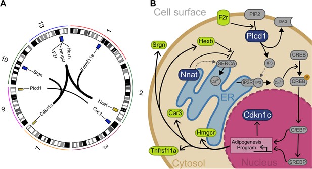
Interacting genes form a diet-responsive network affecting adipogenesis.
(A) There are nine significant imprinting-by-imprinting epistatic ASE/DE/phenotype sets in the F16 advanced intercross population (n = 1002). Interactions are shown as lines connecting ASE (yellow) and DE genes (purple). Chromosome number is shown around the plot. (B) The epistatic parent-of-origin effect network is comprised of key steps in a putative pathway regulating differentiation and survival of adipocytes. This pathway was constructed by incorporating previously published cellular functions. The pathway members are color coded in blue for ASE genes (Plcd1, Nnat, and Cdkn1c) and green for DE genes (F2r, Hexb, Hmgcr, Car3, Tnfrsf11a, and Srgn). The network breaks down into potentiation, transduction, and response. Nnat and Hexb potentiate signaling by managing availability and accumulation of calcium necessary for signal transduction. Once a signal is received, F2r and Plcd1 transduce it by activating second messengers to initiate a response. This response initiates an adipogenesis cellular program that affects expression of Cdkn1c, Hmgcr, Car3, Tnfrsf11a, and Srgn.
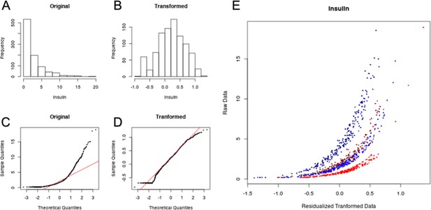
Example transformation of F16 phenotypes.
In order to meet the assumptions of normality required by ANOVAs, non-normally distributed phenotypes were log transformed and residualized to remove the effects of sex and diet. Normality was evaluated by Shapiro-Wilkes test (p < 0.05 indicates non-normality). Serum insulin is one such phenotype. The probability distribution of serum insulin is shown before (A) and after transformation (B). This distribution is also compared to a normal distribution via quantile-quantile plot before (C) and after (D) transformation. The removal of sex and diet effects on serum insulin are shown (E) for high-fat males (dark blue), low-fat males (light blue), high-fat females (dark red), low-fat-fed females (light red).
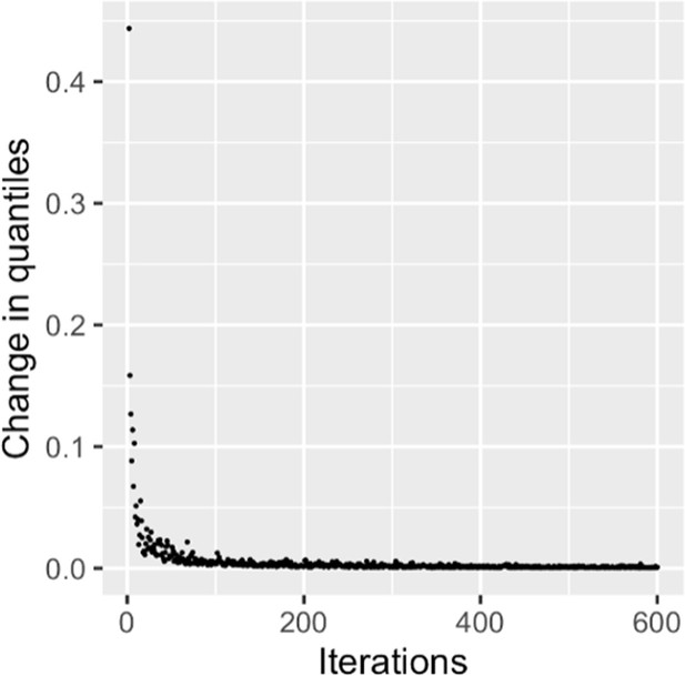
Stable null permutations plot for epistasis.
Imprinting scores were permuted to generate an appropriate null model p-value. Null distribution stability was evaluated by calculating the total quantile deviation (TQD) at each iteration. The TQD of F-statistics under the null model approaches zero over 600 iterations.
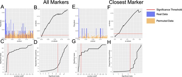
Representative multiple tests correction of imprinting:imprinting epistasis.
Multiple test corrections was performed on each phenotype individually. Here were show this for the GTT area under the curve at 10 weeks phenotype using both all markers within 1.5 Mb (A–D) and only the nearest marker (E–H). Multiple tests correction was performed by estimating the false discovery rate using a permuted null model of p-values. Imprinting scores were permuted to generate an appropriate null model p-values. The distribution of permuted (orange) and real (blue) p-values is shown (A and E). False discovery rate was estimated as the proportion of tests below a given significant threshold under the null relative to the real data (Null/Real). A ratio of 1 meaning that ~100% of observations at that significance threshold are likely false discoveries. The relationship between false discovery rate and p-value threshold is shown (B and F). The number of significant tests at a given acceptable false discovery rate is shown (C and G). The number of false positives relative to the number of significant tests is shown (D and H).
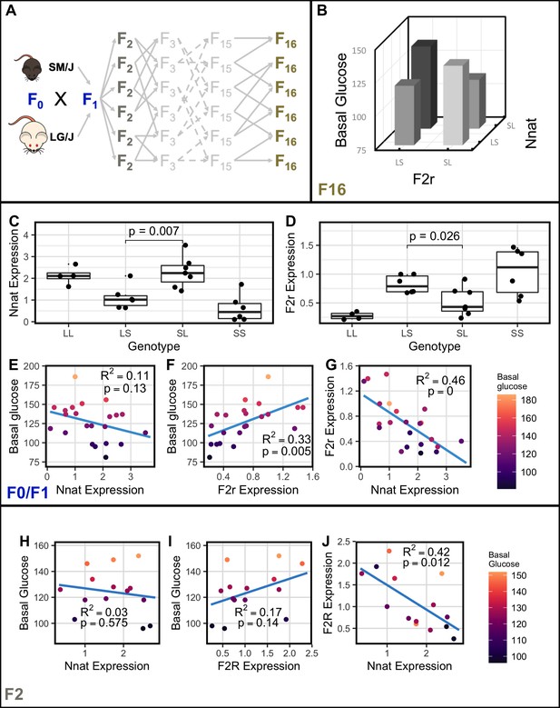
Nnat and F2r covary across generations.
(A) Breeding scheme for the F16 Advanced Intercross between the LG/J and SM/J inbred strains. (B) Significant imprinting-by-imprinting epistasis associated with variation in basal glucose (n = 1002). The parent-of-origin effects of F2r on basal glucose depend on the parent-of-origin effects at Nnat. (C) Expression of Nnat across genotypes in a combined F0/F1 population of high fat-fed females (n = 25). (D) Expression of F2r across genotypes in a combined F0/F1 population of high-fat-fed females (n = 25). (E) Significant correlation between Nnat and F2r expression in the F0/F1 mice (F1 n = 13; F0 n = 12). (F) and (G) Correlations between basal glucose and Nnat and F2r in the F0/F1 mice (F1 n = 13; F0 n = 12). (H) Significant correlation between Nnat and F2r expression in the high fat-fed female F2 mice (n = 14). (I) and (J) Correlations between basal glucose and Nnat and F2r are not individually significant in the F2 mice. Alleles are ordered maternal | paternal within the genotype classes.
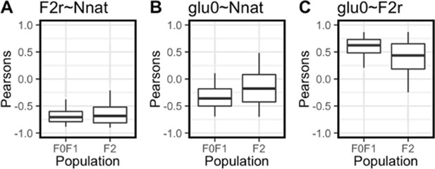
Pearson’s correlation coefficient confidence intervals.
To determine whether the pattern of correlations is significantly different between F0/F1 and F2 populations bootstrapping was employed (N = 10, 5000 iterations). Pickets correspond to 90% confidence intervals, boxes correspond to 50% confidence intervals. Overlap of confidence intervals indicates no significant difference between populations. Correlation between F2r and Nnat expression is not significantly different (A). Correlation between Nnat and basal glucose is not significantly different (B). Correlation between F2r and basal glucose is not significantly different (C).
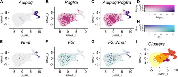
Nnat expression increases and F2r expression decreases in pre-adipocytes along an adipogenic trajectory.
(A) Adipoq is a marker of adipocytes whose expression (purple) increases along the trajectory. (B) Pdgfra is a marker of mesenchymal stem cells whose expression (pink) decreases along the trajectory. (C) Cells in clusters expressing one or both Adipoq and Pdgfra fall along an adipogenic trajectory. (D) Intensity of expression of Adipoq and Pdgfra indicated by coloration. (E) Nnat expression (blue) increases along the trajectory. (F) F2r expression (teal) decreases along the trajectory. (G) Negative association between Nnat and F2r expression within adipocytes along the trajectory. (H) Intensity of expression of Nnat and F2r indicated by coloration. (I) The adipogenic trajectory is broken into subclusters of cells with no Adipoq expression (cluster 0) to high Adipoq expression (cluster 2).
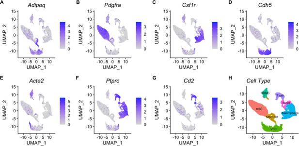
Cell types were defined using canonical markers.
Expression of these markers is shown by coloration on UMAP plots for Adipoq = differentiating mesenchymal stem cells (A); Pdgfra = mesenchymal stem cells (B); Csf1r = macrophage(C); Cdh5 = vascular endothelial cells(D); Acta2 = vascular smooth muscle cells(E); Ptprc – T cells(F); Cd2 – B cells (G). Cell type identities were assigned by expression of these genes (H).
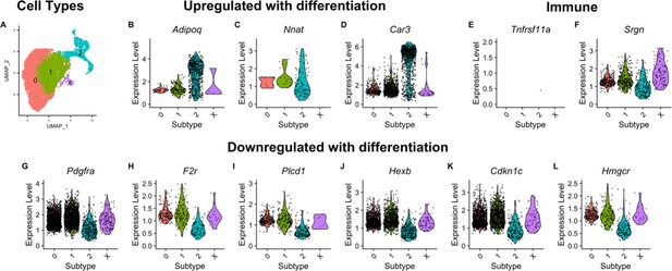
Candidate genes are differentially expressed across adipogenic trajectory.
Cells along the adipogenic trajectory were clustered into 4 groups [0, 1, 2, X](A). Adipogenic trajectory was defined by the expression of Adipoq in differentiation MSC (B) and by Pdgfra in undifferentiated MSC (G). Expression of candidate genes identified by integrating F0/F1 RNAseq with F16 data is shown. Only cells with non-zero expression are plotted. Two candidate genes are primarily expressed by immune cells (E and F), but one of which is differentially expressed along the adipogenic trajectory (F). Two candidate genes are primarily expressed along the trajectory and are upregulated with differentiation (C and D). Five candidate genes are primarily expressed along the trajectory and downregulated with differentiation (H–L).
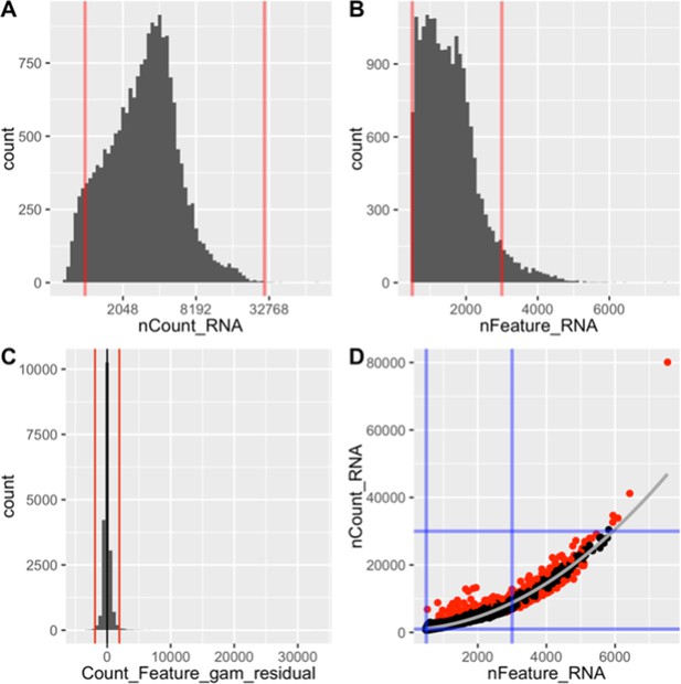
Single cell quality was controlled.
The number of counts for a given gene in a given cell nCount (A), the number of genes expressed in a given cell nFeature (B), and their covariation (C) is predictive of cell quality. The strength of their relationship was measured as the residual for each cell in a generalized additive model predicting nCount from nFeature. Thresholds for these metrics (red/blue lines) were used to decide which cells to include. Cells with unacceptably high residuals (red dot) were thrown out.
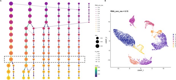
Determining the resolution for clustering.
Dimensionality reduction of high dimensional single-cell RNAseq data requires the selection of a resolution parameter. This parameter is selected by seeing how stable cluster number and assignment is across a range of resolution parameter values as shown on a cluster tree (A). Here, we selected the highest resolution parameter that stably clustered the expected cell populations. The selected value was 0.15. Using this value, dimensionality reduction is visualized using the UMAP method (B). Cluster identifiers is consistent between cluster tree and UMAP projection.
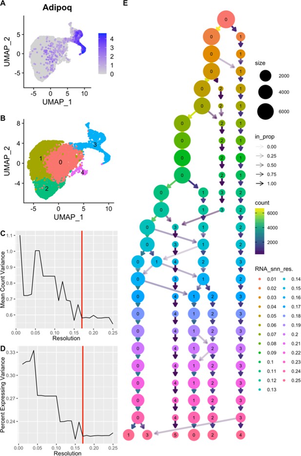
Adipocyte clustering resolution was selected to minimize Adipoq variation.
We sought to test for differential expression of genes across the adipogenic trajectory. Cells from the trajectory were subset and re-clustered. We sought to cluster cells into groups that best corresponded to the different stages of differentiation (B). To this end we used Adipoq expression as a marker of differentiation (A). This dimensionality reduction of high dimensional single-cell RNAseq data requires the selection of a resolution parameter. We tested a range of resolution parameters from 0.01 to 0.25 and observed how resolution affected clustering (E). For each resolution parameter, the variation in mean variation in non-zero Adipoq expression within all clusters was calculated (C). The same was done to calculate the mean variation in percent of cells with expression >0 within all clusters. By finding the clustering conditions that in which Adipoq expression was stably minimized, we were able to select the resolution parameter that best clustered cells into the different stages of differentiation (resolution = 0.17). Dimensionality reduction is visualized using the UMAP method (B). Cluster identifier is consistent between cluster tree and UMAP projection.
Tables
| Reagent type (species) or resource | Designation | Source or reference | Identifiers | Additional information |
|---|---|---|---|---|
| Other | High fat diet | Teklad | TD88137 | 42% kcal from fat |
| Other | Low-fat diet | Research Diets | D12284 | 15% kcal from fat |
| Commercial assay, kit | RNeasy Lipid Tissue Kit | QIAgen | 74,804 | |
| Commercial assay, kit | RiboZero kit | Illumina | 20040529 | |
| Commercial assay, kit | DNA 1000LabChip | Agilent | 5067–1504 | |
| Commercial assay, kit | High-Capacity cDNA Reverse Transcription Kit | Thermo Fisher | 4368814 | |
| Sequence-based reagent | Nnat forward primer | This paper | Detailed information is found in the methods section | |
| Sequence-based reagent | Nnat reverse primer | This paper | Detailed information is found in the methods section | |
| Sequence-based reagent | F2r forward primer | This paper | Detailed information is found in the methods section | |
| Sequence-based reagent | F2r reverse primer | This paper | Detailed information is found in the methods section | |
| Sequence-based reagent | L32 forward primer | This paper | Detailed information is found in the methods section | |
| Sequence-based reagent | L32 reverse primer | This paper | Detailed information is found in the methods section | |
| Software, algorithm | R | R | 3.6.1 | |
| Software, algorithm | STAR | STAR | DOI: 10.1093/bioinformatics/bts635 | |
| Software, algorithm | FASTQC | FASTQC | other | https://www.bioinformatics.babraham.ac.uk/projects/fastqc/ |
| Software, algorithm | EdgeR | CRAN | DOI: 10.1093/bioinformatics/btp616 | |
| Software, algorithm | WEB-based Gene Set Analysis Toolkit | WEB-based Gene Set Analysis Toolkit | DOI: 10.1093/nar/gkz401 | |
| Software, algorithm | Seurat | Seurat | DOI: 10.1038/nbt.3192 | |
| Strain, strain background (Mus musculius) | SM/J | The Jackson Laboratory | 000687 | |
| Strain, strain background (Mus musculus) | LG/J | The Jackson Laboratory | 000675 |
Additional files
-
Supplementary file 1
Allele-specific expression.
- https://cdn.elifesciences.org/articles/72989/elife-72989-supp1-v2.xlsx
-
Supplementary file 2
Biallelic genes differentially expressed by cross.
- https://cdn.elifesciences.org/articles/72989/elife-72989-supp2-v2.xlsx
-
Supplementary file 3
Networks of genes showing parent-of-origin allele-specific expression interacting with biallelic genes that are differentially expressed by cross.
- https://cdn.elifesciences.org/articles/72989/elife-72989-supp3-v2.xlsx
-
Supplementary file 4
Over-representation input/output.
- https://cdn.elifesciences.org/articles/72989/elife-72989-supp4-v2.xlsx
-
Supplementary file 5
F1 Phenotype correlation.
- https://cdn.elifesciences.org/articles/72989/elife-72989-supp5-v2.xlsx
-
Supplementary file 6
Epistasis results.
- https://cdn.elifesciences.org/articles/72989/elife-72989-supp6-v2.xlsx
-
Supplementary file 7
Cell cluster markers.
- https://cdn.elifesciences.org/articles/72989/elife-72989-supp7-v2.xlsx
-
Supplementary file 8
Alignment summaries.
- https://cdn.elifesciences.org/articles/72989/elife-72989-supp8-v2.xlsx
-
Supplementary file 9
List of imprinted genes queried.
- https://cdn.elifesciences.org/articles/72989/elife-72989-supp9-v2.xlsx
-
Supplementary file 10
Genome annotations.
- https://cdn.elifesciences.org/articles/72989/elife-72989-supp10-v2.xlsx
-
Transparent reporting form
- https://cdn.elifesciences.org/articles/72989/elife-72989-transrepform1-v2.docx


