Analysis of rod/cone gap junctions from the reconstruction of mouse photoreceptor terminals
- Richard Ruiz Department of Ophthalmology and Visual Science, McGovern Medical School, University of Texas at Houston, United States
- Department of Chemical Physiology & Biochemistry, Oregon Health & Science University, United States
- Department of Biology, University of Maryland, College Park, United States
- Retinal Neurophysiology Section, National Eye Institute, National Institutes of Health, United States
Figures
Figure 1 with 1 supplement
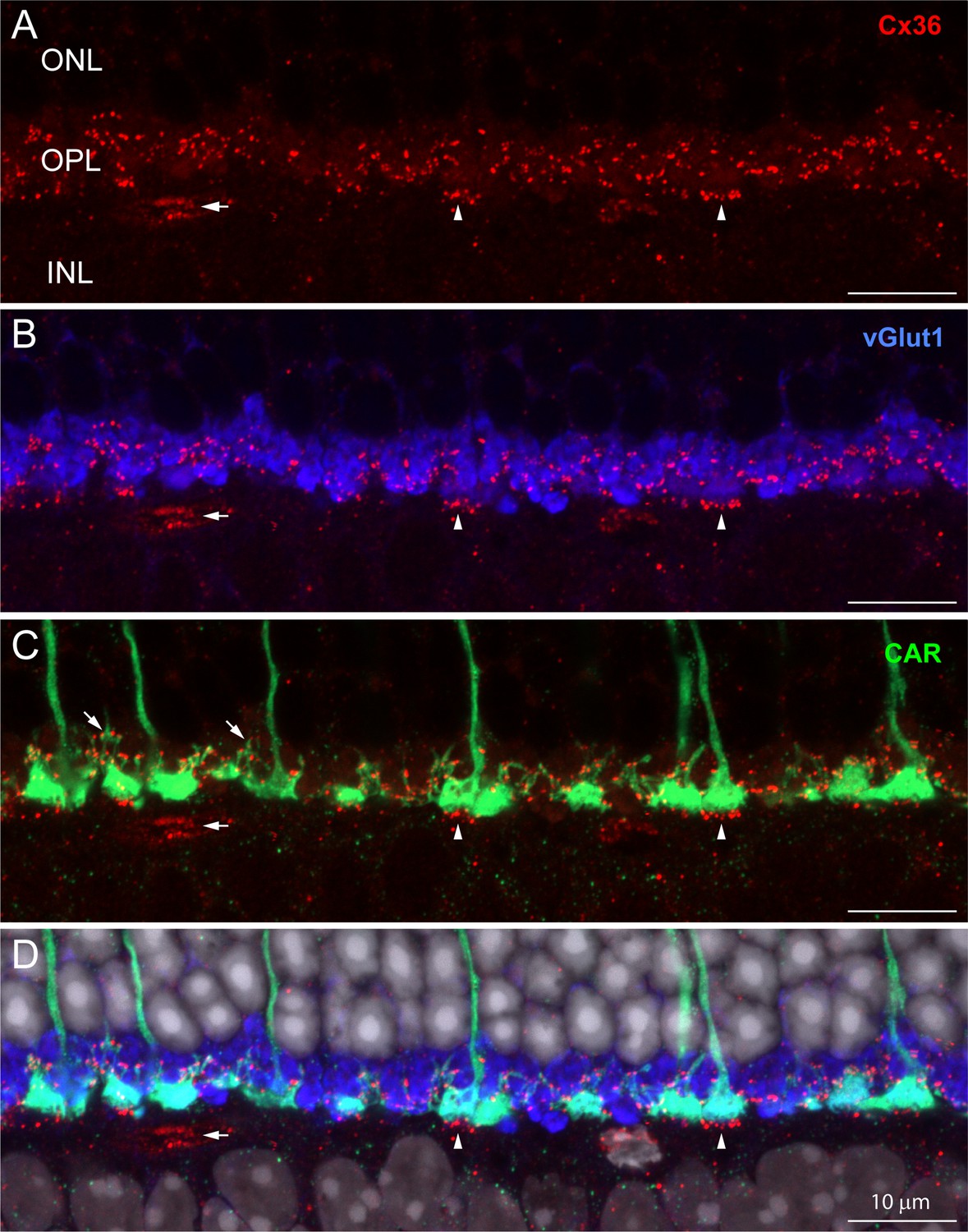
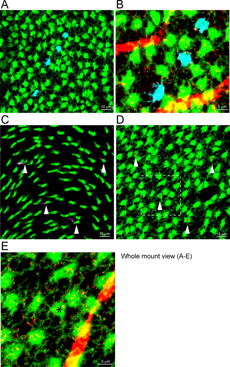
The distribution of Cx36 in the outer plexiform layer (OPL).
Cx36 labeling in the OPL, confocal microscopy. (A) Numerous small Cx36 clusters (red) restricted to the OPL, absent in the outer nuclear layer (ONL). For all four panels: horizontal arrowheads, bipolar cell Cx36 clusters under each cone pedicle that were excluded from analysis because they were not colocalized with cone pedicles; horizontal arrow, non-pecifically labeled blood vessel. (B) Cx36 clusters are contained within the band of rod spherules, stained with an antibody against vGlut1 (blue). (C) Cx36 clusters decorate the cone pedicles and their telodendria, labeled for cone arrestin (green). Oblique arrows point to examples of cone telodendria. (D) Four channels showing Cx36 (red), cone pedicles (green), and rod spherules (blue) all contained within the OPL. DAPI-labeled nuclei (gray) show the well-organized ONL. Figure 1—video 1 shows this dataset.
Figure 1—video 1
Animation of a confocal series from the outer plexiform layer (OPL) showing Cx36 (red) decorating the cone telodendria (green, cone arrestin).
All Cx36 clusters fall within the band of vGlut1 (blue)-labeled rod spherules. No Cx36 in the outer nuclear layer (ONL).
Figure 2 with 5 supplements
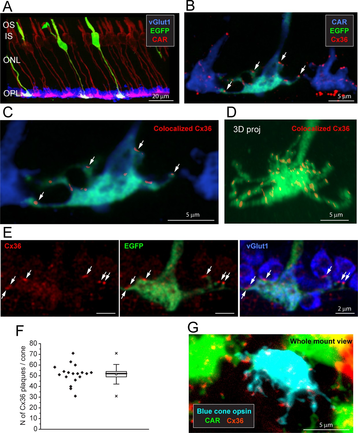
Cx36 is colocalized with cone pedicles.
(A) EGFP-labeled single cones (green) against a background of all cones stained for cone arrestin (red) and vGlut1, which stains rod spherules (blue). Most cone pedicles appear magenta because they are labeled for both cone arrestin and vGlut1. The EGFP-labeled cone pedicles are white, triple labeled for EGFP, cone arrestin, and vGlut1. (B) A mini-stack of five optical sections (0.5 μm in total) showing the distribution of Cx36 (red) on cone pedicles (blue), including a single EGFP-labeled cone (green + blue = cyan). Arrows point to individual Cx36 clusters. Images of individual channels are available in Figure 2—figure supplement 1A. (C) Enlarged version, same mini-stack showing Cx36 clusters colocalized with the single EGFP-labeled cone pedicle. Note the similarity with panel (B) because Cx36 is predominantly colocalized with cone pedicles and there is very little nonspecific Cx36 background. Additional images of the same size as (B) are available in Figure 2—figure supplement 1B. (D) 3D projection of a complete single EGFP cone pedicle (green) compiled from confocal sections showing only Cx36 clusters (red) colocalized with this cone pedicle, as in (C). From such data, we calculated the mean number of Cx36 clusters per cone pedicle (F, below). Images of individual channels are available in Figure 2—figure supplement 1C. Figure 2—video 1 shows this dataset. (E) A single confocal section showing that rod spherules (blue) occur close to the Cx36 clusters (red) located on a cone pedicle (green). Left: Cx36 clusters (red), arrows point to individual Cx36 clusters (all panels). There is some faint background labeling for Cx36, which is mostly contained within the cone pedicle. Center: the distribution of Cx36 clusters (red) on a cone pedicle (green) and its telodendria. Right: triple label showing that rod spherules, labeled for vGlut1 (blue), contact the cone pedicle (green +blue = cyan) at Cx36 clusters (red). (F) The number of Cx36 clusters, 51.4 ± 8.88 (mean ± SD), on a single reconstructed cone pedicle (as in D), box shows quartiles, mean (circle), median (bold line), SD (whisker), min/max (x), n = 18. (G) Blue cone pedicle (cyan), identified in a blue cone opsin Venus mouse line, had telodendria-bearing Cx36 clusters (red), similar to those of green cones, stained for cone arrestin (green).
-
Figure 2—source data 1
Number of Cx36 clusters on a single-cone pedicle.
Source data for Figure 2F.
- https://cdn.elifesciences.org/articles/73039/elife-73039-fig2-data1-v3.xlsx
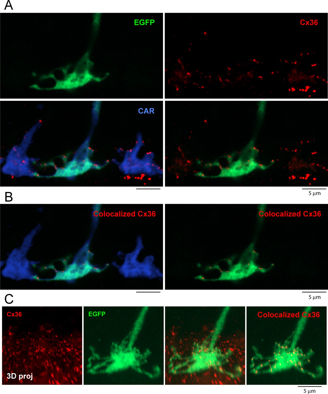
Figure 2—figure supplement 1
3D reconstruction of a single EGFP-labeled cone pedicle and colocalized Cx36 clusters.
(A) Top left: a single EGFP-labeled cone pedicle (green), five optical sections, total 0.5 μm thickness, Airyscan. Top right: same field showing Cx36 clusters (red). Lower left: all cones labeled for cone arrestin (blue), single EGFP cone pedicle is green + blue = cyan, Cx36 clusters (red) are colocalized with cone pedicles, except for those underneath each cone pedicle, which are not included in the analysis. Lower right: single EGFP-labeled cone pedicle with Cx36 clusters. Some of the Cx36 clusters are located on the EGFP-labeled cone pedicle. (B) Left: cone pedicles labeled for cone arrestin (blue) and a single EGFP-labeled cone (green + blue = cyan) with Cx36 (red) colocalized with the EGFP-labeled cone. Right: the single EGFP-labeled cone pedicle with only the Cx36 clusters colocalized with this cone pedicle. (C) Left: confocal projection of Cx36 clusters (red) in the outer plexiform layer (OPL). Center left: 3D projection of a single EGFP-labeled cone pedicle. Center right: the same EGFP-labeled cone with all the Cx36 labeling in the OPL. Right: 3D projection of the same cone pedicle (green) with only the Cx36 clusters (red) colocalized with this cone.
Figure 2—figure supplement 2
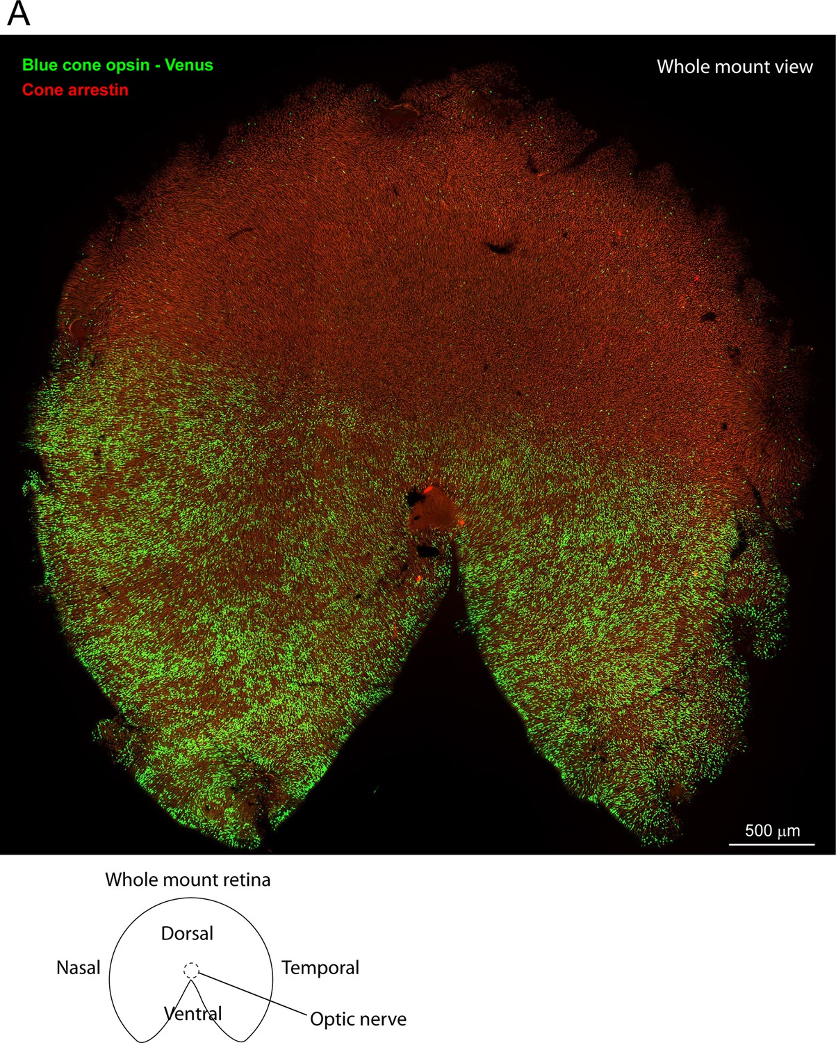
The distribution of blue cone opsin in the mouse retina.
(A) Wholemount view of whole blue cone opsin Venus mouse retina shows most cones in ventral retina express blue cone opsin. In the dorsal retina, there is a sparse mosaic of true blue cones.
Figure 2—figure supplement 3
Blue cone pedicles have telodendria-bearing Cx36 clusters.
(A) Dorsal retina of a blue cone opsin Venus mouse contains a sparse set of true-blue cones (cyan) among the majority of green cones labeled for cone arrestin (green). (B) Zoom-in on one blue cone pedicle shows Cx36-labeled (red) telodendria. Surrounding green cone pedicles labeled for cone arrestin (green). Large red structures are nonspecifically labeled blood vessels. (C) Outer segments showing a sparse set of cones labeled with an antibody against blue cone opsin (magenta). Background of green cones labeled for cone arrestin (green). (D) Following the cone axons through a series of confocal images allows the blue cone pedicles to be identified (asterisks), see Figure 2—video 2. (E) Enlarged view of a single blue cone pedicle (asterisk) with Cx36 (red)-labeled telodendria, comparable to the surrounding green cones labeled for cone arrestin (green).
Figure 2—video 1
3D reconstruction of a single EGFP-labeled cone pedicle among all cone arrestin (blue)-labeled cones, with extensive telodendria.
All the Cx36 clusters in the outer plexiform layer (OPL), then only those Cx36 clusters, more than 50, colocalized with the single EGFP-labeled cone pedicle. Cx36 is distributed along the telodendria, often at the tips, and on the upper surface or roof of the cone pedicle.
Figure 2—video 2
Animating from the outer plexiform layer (OPL) to the outer segments following the cone axon allows cone labeled for blue cone opsin (magenta) to be connected to its pedicle (*), labeled for cone arrestin.
Figure 3 with 1 supplement
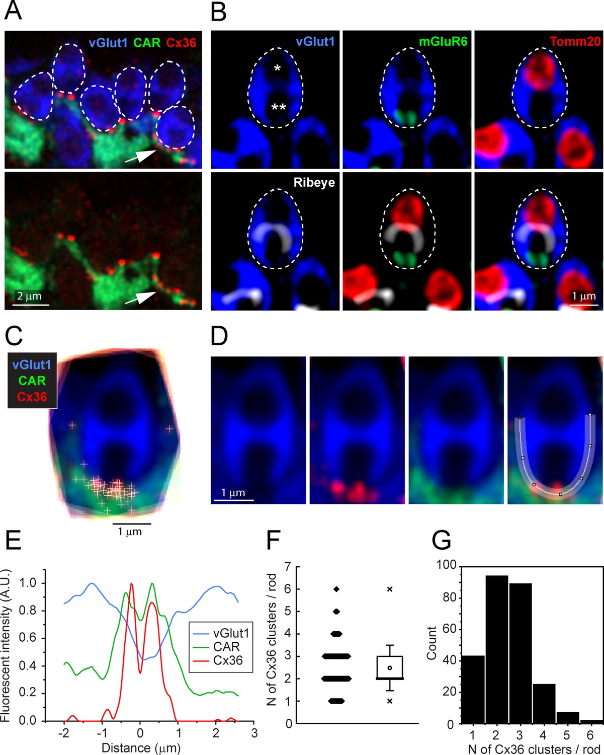
Cx36 clusters are found at the base of each rod spherule.
(A) Top: details of outer plexiform layer (OPL), rod spherules, stained for vGlut1 (blue) and outlined with dashed lines are located above and between cone pedicles labeled for cone arrestin (green). Cx36 clusters (red) are found at the base of rod spherules where they contact cones. Multiple Cx36 clusters occur at some contacts (arrow). Bottom: Cx36 clusters are located on cone telodendria. Images of individual channels are available in Figure 3—figure supplement 1A. (B) Top left: a rod spherule labeled for vGlut1 (blue), outlined with a dashed line, has two compartments (* and **). Top middle: bottom compartment is open at the base and contains two mGluR6-labeled rod bipolar dendrites, identifying the postsynaptic compartment. Top right: the upper compartment is filled with a large mitochondrion, labeled for TOMM20 (red). Lower left: the synaptic ribbon, labeled for ribeye (white), lies between the two compartments, arching over the postsynaptic compartment. Lower middle: the synaptic ribbon lies between the mitochondrion and the mGluR6 label. Bottom right: all four labels superimposed showing a typical rod spherule. Images of individual channels with visible background are available in Figure 3—figure supplement 1B. (C) 18 rod spherules, each from one optical section, aligned and superimposed. Taking the rod spherule as a clock face (top center is 12 o’clock), Cx36 clusters (red with individual puncta marked +), are found at the base, 6 o’clock, along with cone telodendria (green). The two single +s at 3 o’clock and 9 o’clock are associated with other rod spherules and were excluded from the analysis. (D) Average rod spherule showing Cx36 and cone telodendria at the base with a fitted spline curve. (E) The distribution of label in each confocal channel along a linearized version of the spline curve. Where the vGlut1 label is low, indicating the opening to the postsynaptic compartment, the Cx36 (red) and cone (green) signals are high. The double peak for Cx36 indicates clusters on each side of the synaptic opening. (F) Scatterplot showing the number of Cx36 clusters, presumed to be gap junctions, per rod spherule from a sample of 260 rods, mean 2.48 ± 1.01, box shows quartiles, mean (circle), median (bold line), SD (whisker), min/max (x). (G) Data plotted as histogram showing the distribution of multiple Cx36 clusters per rod spherule, n = 260 rods, 645 gap junction points.
-
Figure 3—source data 1
Number of Cx36 clusters on a rod spherule.
Source data for Figure 3F and G.
- https://cdn.elifesciences.org/articles/73039/elife-73039-fig3-data1-v3.xlsx
Figure 3—figure supplement 1
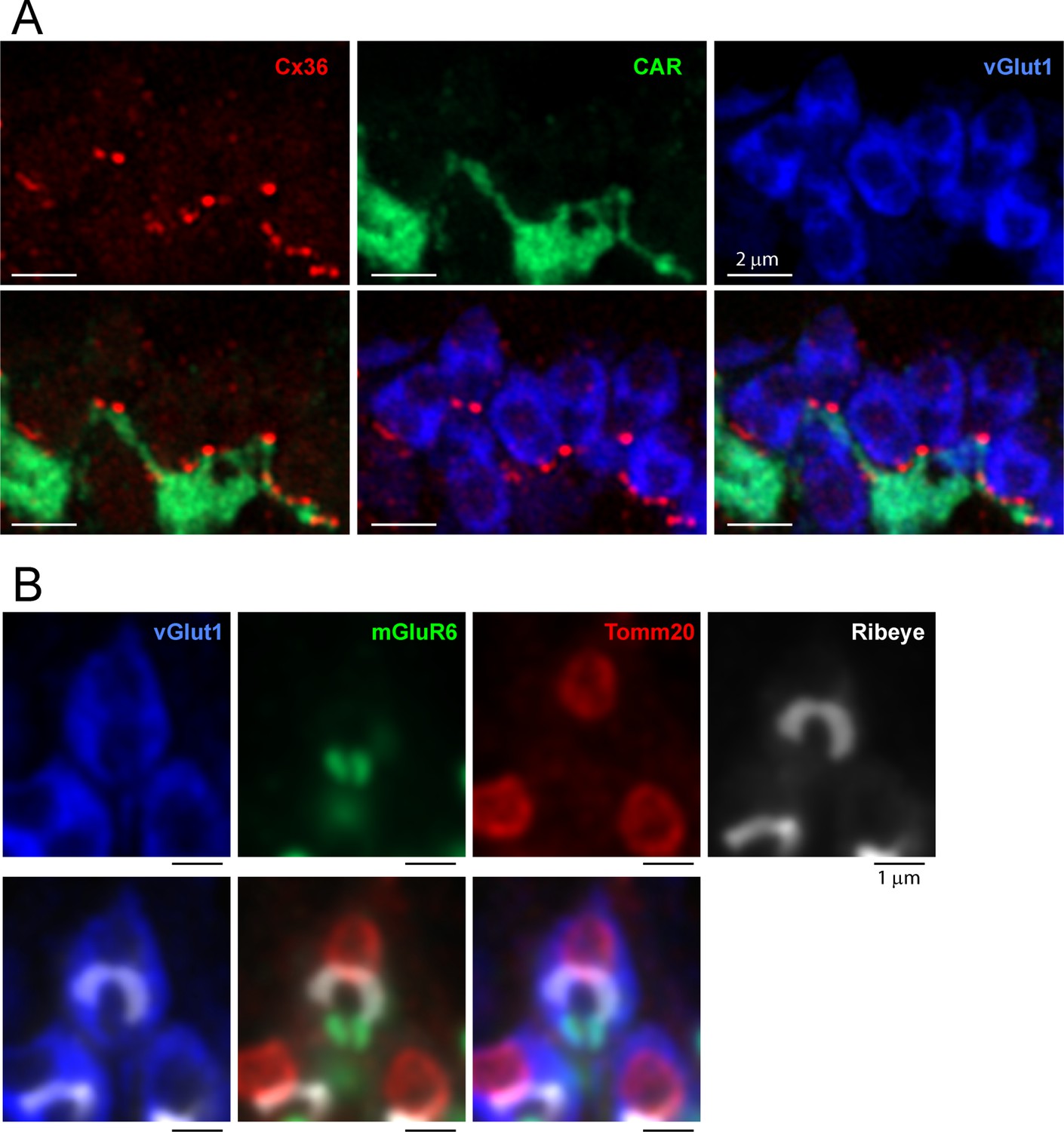
Location of Cx36 and the fine structure of rod spherules.
(A) Single-channel images and double-label combinations of Figure 3A to show background of individual channels. Cx36 clusters (red) are located on cone telodendria (green) at contact points with the base of each rod spherule (blue). Rod spherules were stained with a synaptic vesicle marker, vGlut1. They appear as oval structures with two compartments; the upper compartment contains a large mitochondrion and the lower invagination contains the postsynaptic processes. (B) Detail of an individual rod spherule. Single-channel images and combinations from Figure 3B to show the background of individual channels. A single rod spherule contains two compartments, the upper containing a large mitochondrion stained for TOMM20 (red). The lower compartment contains the postsynaptic processes including two mGluR6 (green)-labeled tips of rod bipolar dendrites. The two compartments are separated by the synaptic ribbon (white), which forms a horseshoe dividing the two compartments in this optimally oriented image.
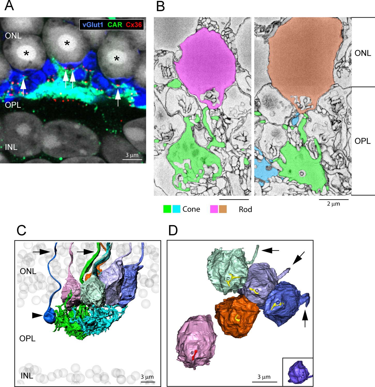
Figure 4
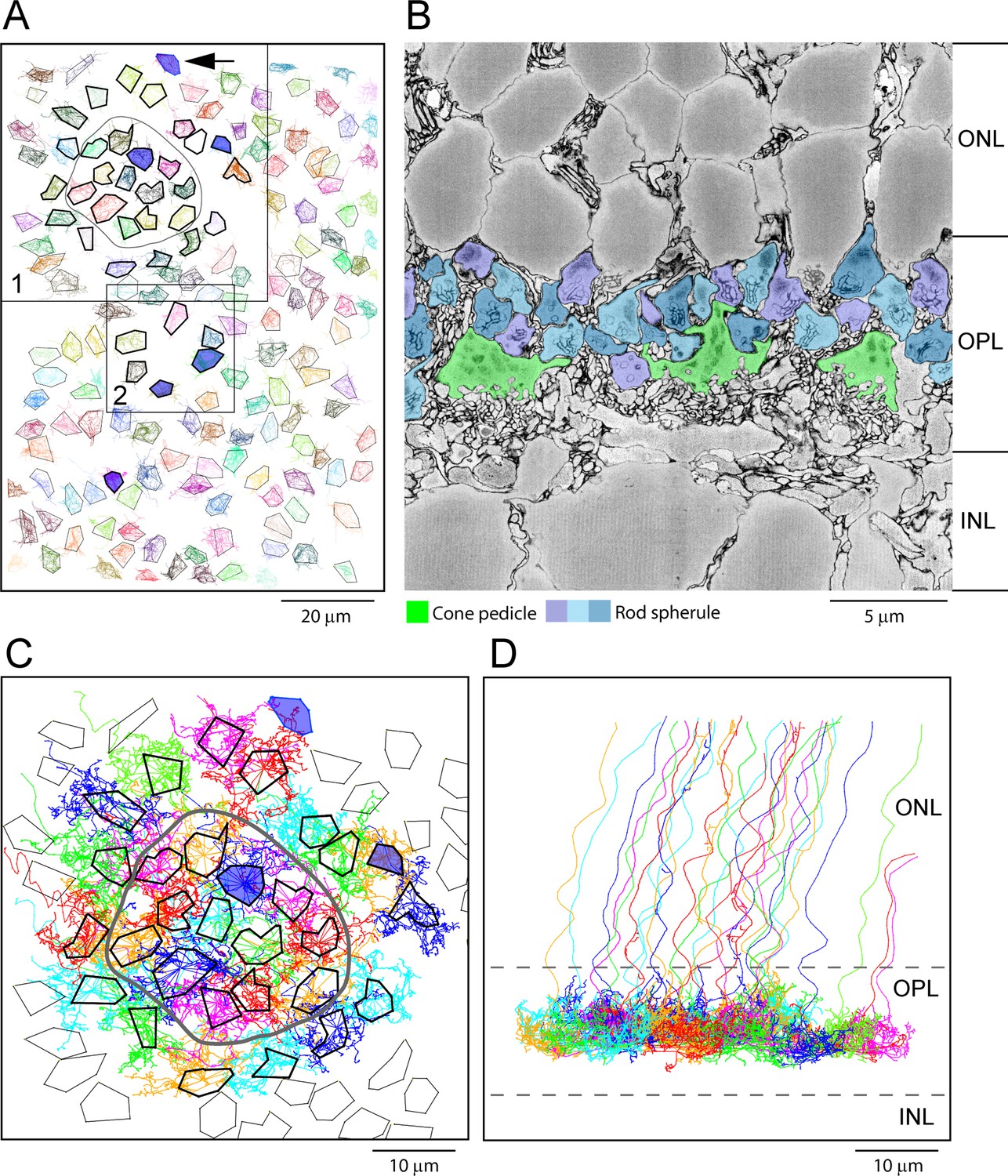
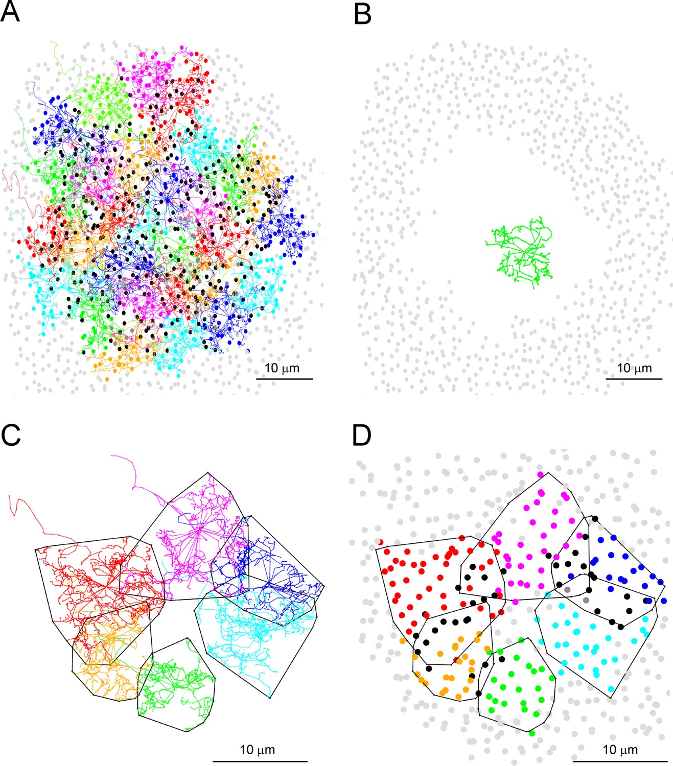
Map of cone pedicles shows telodendria overlap.
(A) Map of 164 cone pedicles in e2006, modified from Behrens et al., 2016. Box 1 contains the 29 cone pedicles (thick outlines) that were reconstructed as skeletons in (C). The central 13 cone pedicles are contained within the ring. Blue cone pedicles filled with dark blue. Box 2 is a lower density area where six additional cone pedicles were also reconstructed as a check (Figure 5—figure supplement 1C). In total, there were six blue cone pedicles, filled dark blue (Behrens et al., 2016). One blue cone pedicle was at the upper edge (black arrow). The cone pedicles outside the boxes were not reconstructed, except for the single blue cone pedicle that lies outside the boxes. (B) Low-power vertical section from e2006 showing rod spherules (three shades of blue), above and in between cone pedicles (green). (C) Skeletons of all 29 reconstructed cone pedicles (thick outlines) showing overlapping telodendrial fields, individually colored. Thick outlines show solid part of cone pedicles. The central 13 cone pedicles are contained within the ring. (D) Projection of (C) showing cone pedicles restricted to the outer plexiform layer (OPL) and axons ascending through the outer nuclear layer (ONL).
-
Figure 4—source data 1
Cone pedicle skeletons and rod spherule points.
- https://cdn.elifesciences.org/articles/73039/elife-73039-fig4-data1-v3.zip
Figure 5 with 2 supplements
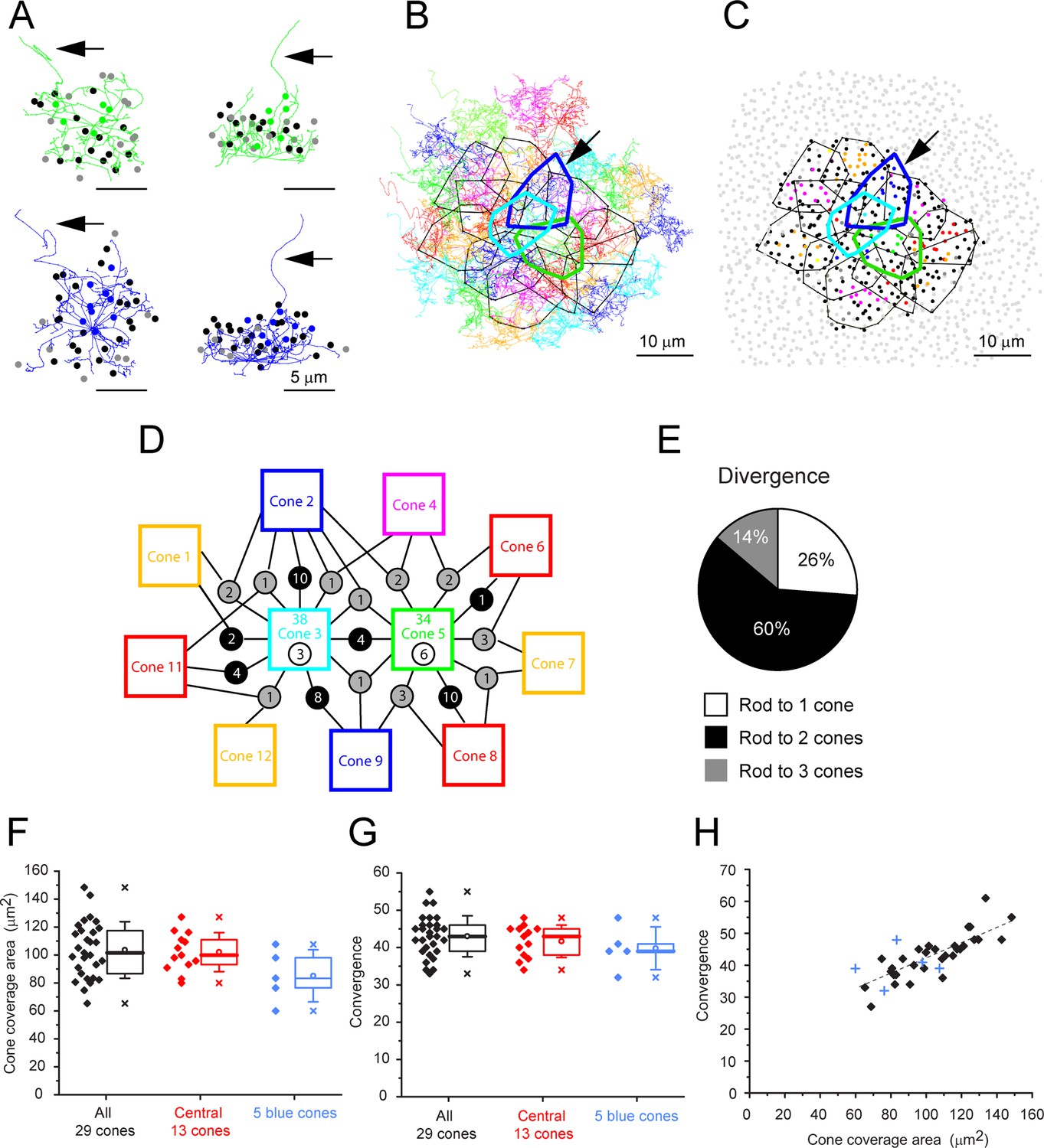
Cone skeleton analysis shows cones contact all nearby rod spherules.
(A) Skeletons of one green cone (cone 5, green) and one blue cone (cone 2, blue) in wholemount view and projected. Black arrows show ascending axons. The position of each contacted rod spherule is marked by a dot, color-coded the same color (green or blue) if the contacts are exclusive to this cone pedicle; black, contacts two cones; gray, contacts three cones. (B) Telodendrial fields of 29 reconstructed cone pedicles, each color-coded; central 13 outlined by polygons, arrow points to blue cone (cone 2, thick blue outline). Cones 3 and 5 are also outlined with cyan and green, respectively. (C) Outlines of central 13 cone pedicles showing all rod spherule contacts, color-coded, exclusive to one cone; black, contacts with two cones; dark gray, contacts with three cones. Light gray, rod spherules outside the range of the central 13 cone pedicles. Arrow points to blue cone (cone 2, thick blue outline). (D) Simplified skeleton map showing contacts of two green cone pedicles (cones 3 and 5); the box contains the cone identity, the total number of rod contacts (above), and the exclusive number of rods that contact this cone only (below). Circles indicate the number of rod spherules shared between cones linked by lines to neighbors. Cone 2 is a blue cone, which shares rod contacts with neighboring cones. (E) Pie chart showing distribution of cone contacts per rod spherule. (F) Area of telodendrial field for all 29 reconstructed cone pedicles, central 13 cones (ring in Figure 4A and C) and 5 blue cones. Box shows quartiles, mean (circle), median (bold line), SD (whisker), min/max (x). (G) Convergence, rod contacts per cone for all 29 reconstructed cone pedicles, central 13 (ring in Figure 4A and C) and five blue cones. Box shows quartiles, mean (circle), median (bold line), SD (whisker), min/max (x). (H) Convergence vs. cone pedicle area. Line of linear regression shows some tendency for larger cone pedicles to contact more rods. +, blue cones.
-
Figure 5—source data 1
Cone coverage area and rod convergence.
Source data for Figure 5F–H.
- https://cdn.elifesciences.org/articles/73039/elife-73039-fig5-data1-v3.xlsx
-
Figure 5—source data 2
The number of rod spherules shared between two adjacent cone pairs.
Source data for Figure 5—figure supplement 2B.
- https://cdn.elifesciences.org/articles/73039/elife-73039-fig5-data2-v3.xlsx
Figure 5—figure supplement 1
Nearly all rods receive cone contacts.
(A) Map showing telodendria of all 29 cone pedicles (Figure 4A, box 1), each individually colored; dots mark all rod spherules in contact, same color as cone if contacts are exclusive to one cone; black, contact with two cones; gray, contact with three cones; light gray, no contacts, mostly outside the field of all 29 cones. Within the field of 29 cones, there were 811 rod spherules, of which 808 (99.6%) received cone contacts. 3/811 (0.4%) rod spherules received no cone contacts. (B) Removing cone pedicles and rod spherules in contact with the central 13 cone pedicles leaves a hole with no remaining rod spherules (0/361) inside an annulus of rod spherules outside the field of the central 13 cones. The telodendrial field of cone 5 (green, axon removed) is shown for comparison. (C) Polygons outline the telodendrial fields of six cones in a sparse region (Figure 4A, box 2). In the center, there is a rare hole in the cone coverage, almost like a cone is missing. (D) Removing cones and plotting rod spherules (color-coded by cone for exclusive contacts; black, two cones; dark gray, three cones; light gray, no contacts) reveals 8/175 (4.6%) of rod spherules in the central area with no cone contacts. This may represent a local upper limit of rods without cone contacts since we deliberately chose a sparse area.
Figure 5—figure supplement 2
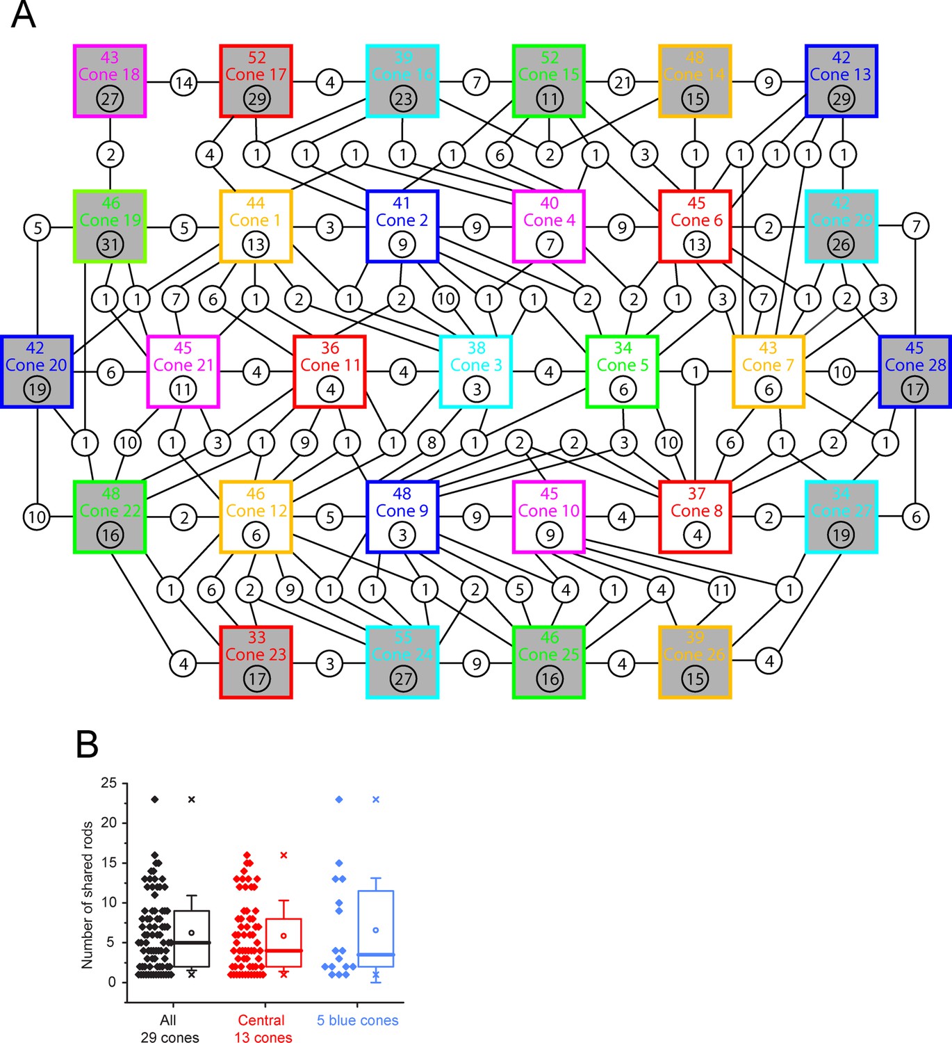
Rod connectivity map for 29 cone pedicles.
(A) Full connectivity map for all 29 cone pedicles that were reconstructed, central 13 clear boxes, outer 16, shaded boxes. Each square represents one cone, containing the identity with the total number of rod contacts above, 43.0 ± 5.40 (mean ± SD, n = 29), and the number of exclusive contacts below, 7.23 ± 3.38 (mean ± SD, n = 13, central cones only; outer cone numbers for exclusive contacts are high due to edge effects). Circles show number of rod spherules shared between cone pedicles connected by lines. Most cone pedicles share rod spherules with all neighboring cones. Cones 5 (green), 3 (cyan), and 2 (blue) were segmented and reconstructed in 3D. Cone 2 is a blue cone (Behrens et al., 2016). (B) The number of rod spherules shared between any two adjacent cone pairs, 6.23 ± 4.67 (mean ± SD, n = 79 pairs among all 29 cones, black), central 13 cones (red), 5.85 ± 4.42 (mean ± SD, n = 61 pairs); blue cones, 6.56 ± 6.34 (mean ± SD, n = 16 pairs from five blue cones). Box shows quartiles, mean (circle), median (bold line), SD (whisker), min/max (x). *79 pairs from the 29 cones include green cone pairs and blue cone–green cone pairs while blue cone data shows blue cone–green cone pairs only. Note that there are no blue cone pairs because they are too widely spaced. Appendix 2—table 2 additionally shows statistics for only green cone pairs, 6.26 ± 4.14 (mean ± SD, n = 69 pairs from 31 green cones) (27 green cones of the 29 cones and 4 green cones in sparse density area).
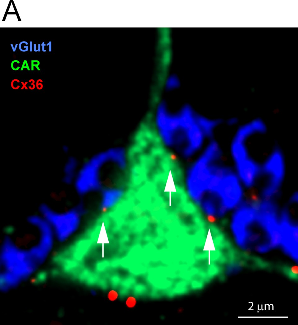
Figure 6 with 7 supplements
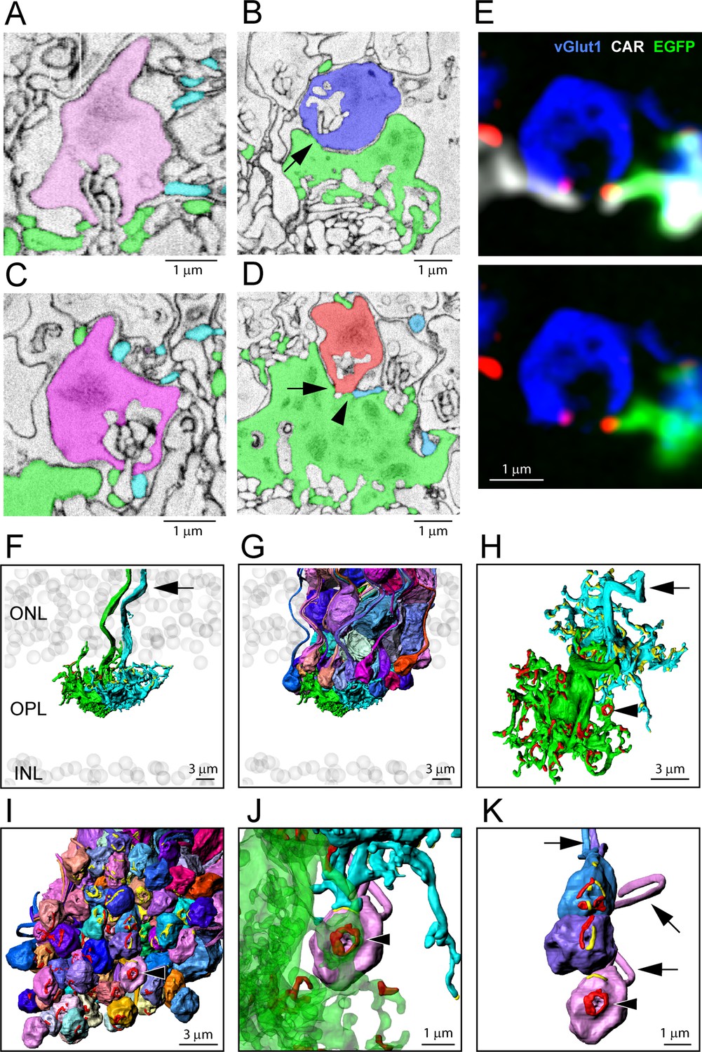
Segmentation and 3D reconstruction e2006: cone telodendria contact rod spherules close to the mouth of the synaptic opening.
(A) Single serial blockface-scanning electron microscopy (SBF-SEM) section, telodendria from two cones (green or cyan), rod spherule (pink), in the plane of the synaptic opening with cone contacts on both sides. (B) Single SBF-SEM section, rod spherule (blue), postsynaptic inclusions show it is close to the synaptic opening, 25 nm × 4 sections = 100 nm away. The rod spherule sits on the roof of a cone pedicle (green) with a contact, shown by the arrow, where membranes merge. (C) Single SBF-SEM section, rod spherule (magenta) with contacts at the synaptic opening from two different cones (green or cyan). (D) Single SBF-SEM section, rod spherule (orange), contacts (arrow) the roof of a cone pedicle (green) with a telodendrial contact (arrowhead) from a second cone (cyan). Postsynaptic inclusions in the rod spherule indicate the contacts are close to the synaptic opening, 25 nm × 9 sections = 225 nm away. (E) Top: confocal microscopy, single optical section, shows Cx36 clusters (red) where telodendria from two different cones (white for cone arrestin, labels both cones; green for a single EGFP-labeled cone) contact rod spherule (blue), at the mouth of the synaptic opening. Bottom: cone arrestin signal turned off for clarity, showing only one cone is labeled for EGFP. (F) 3D reconstruction from e2006, two adjacent green cone pedicles (cone 5, green, and cone 3, cyan), ghost cell bodies (gray) show limits of outer nuclear layer (ONL) and inner nuclear layer (INL), arrow marks ascending cone axons. (G) Same two cone pedicles with all 66 ( = 38 + 34–6 shared) reconstructed rod spherules contacted by these two cones. (H) Rotated view, looking down at top surface of same two cone pedicles, contact pads with rod spherules marked in red or yellow for each cone. Arrowhead marks a single rod spherule; arrow ascending axon. (I) Rotated view, looking up at the bottom surface of all rod spherules in contact with these two cones, contact pads in red or yellow, arrowhead marks a single rod spherule magnified in panels (J) and (K). (J) Single rod spherule (pink), green cone pedicle (cone 5), with adjusted transparency, with contact pad (red) encircling the synaptic opening at the base of the rod spherule (arrowhead). The second cone (cone 3, cyan) also contacts this rod spherule nearby (yellow), approximately 1 μm from the synaptic mouth. (K) Detail showing the bottom surface of three adjacent rod spherules that receive contacts close to the synaptic opening from both cone pedicles, contact pads in red or yellow, arrows show rod axons, arrowhead indicates same rod spherule as (J). Figure 6—video 2 shows this dataset.
Figure 6—figure supplement 1
Confocal microscopy, roof contacts.
(A) Cx36 clusters (red) occur where three rod spherules (vGlut1, blue) make contact (arrows) with the upper surface or roof of a single EGFP-labeled cone (green). Each of these probable gap junctions is close to the opening of a rod spherule postsynaptic compartment.
Figure 6—figure supplement 2
Low rods.
(A) Confocal microscopy, three rod somas, labeled with DAPI (gray, asterisks) in the lowest row of the outer nuclear layer (ONL) adjacent to the upper margin of the outer plexiform layer (OPL), have no axons or spherules. Instead, the synaptic machinery, stained with vGlut1 (blue), is contained in a crescent at the base (Li et al., 2016). Cone telodendria, stained for cone arrestin (green), contact each of these rods with Cx36 clusters (arrows, red) at the contact points, close to the mouth of the synaptic opening. (B) Segmentation from e2006, single sections; left, a rod soma from the lowest row of the ONL contains postsynaptic inclusions at the base and receives contact from a cone telodendron (green) close to the postsynaptic opening (25 nm × 7 sections = 175 nm away); right, a similar example, a low rod soma, (brown) with a postsynaptic compartment at the base receives contacts from two different cones (green and cyan) (16.5 nm × 5 sections = 82.5 nm to the postsynaptic opening). (C) 3D reconstruction of the five rods in the lowest row of the ONL above cones 5 and 3 (a subset of the rods in Figure 6G) shows they sit on a nest of upreaching cone telodendria. For comparison, a rod spherule (blue) is included, far left, arrowhead. Arrows, axon ascending from rod spherule and cone 5 axon (green). (D) The same five low rods rotated to view the cone telodendrial contact pads (yellow or red) around the mouth of the postsynaptic compartment on the lower surface of each rod. Arrows show axons. Inset for size comparison, a reconstructed rod spherule.
Figure 6—figure supplement 3
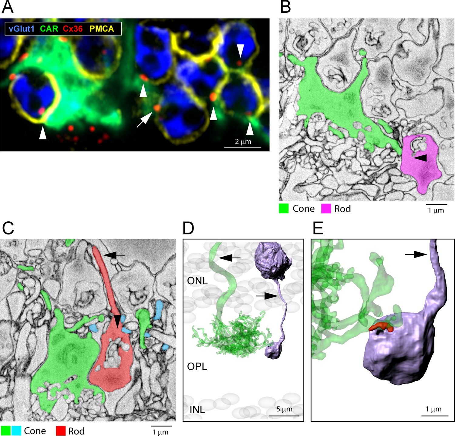
Low rod spherules.
(A) Confocal microscopy, outer plexiform layer (OPL), a cone pedicle, and telodendria stained for cone arrestin (green) and a cluster of rod spherules, stained for vGlut1 (blue) and outlined for plasma membrane calcium ATPase (PMCA) (yellow). Cx36 clusters (red) occur at cone contacts with the base of each rod spherule, close to the synaptic opening (arrowheads). One rod spherule is very low and protrudes below the level of the cone pedicle. This rod spherule is rotated horizontally so the postsynaptic opening is adjacent to the cone pedicle and there is a Cx36 cluster at this contact site (arrow). Thus, the rule is that rod/cone contacts occur close to the rod spherule postsynaptic opening, whatever the orientation. (B) Segmentation, e2006 dataset, a low rod spherule (pink) is inverted to receive a cone contact (green) close to the synaptic opening (arrowhead), 25 nm × 24 frames = 600 nm away. (C) An inverted rod spherule (orange), adjacent to a cone pedicle (green) but with clear membrane separation and no contact, receives cone telodendrial contacts (cyan) near the synaptic opening, (25 nm × 12 frames = 300 nm away), which in this case is uppermost (arrowhead). (D) 3D reconstruction e2006, a low rod spherule (purple) is inverted and receives a cone contact (green, transparent), close to the postsynaptic mouth. Arrows indicate cone axon and rod axon, ascending to rod soma. (E) Detail showing the contact pad (red) curved around the postsynaptic opening.
Figure 6—figure supplement 4
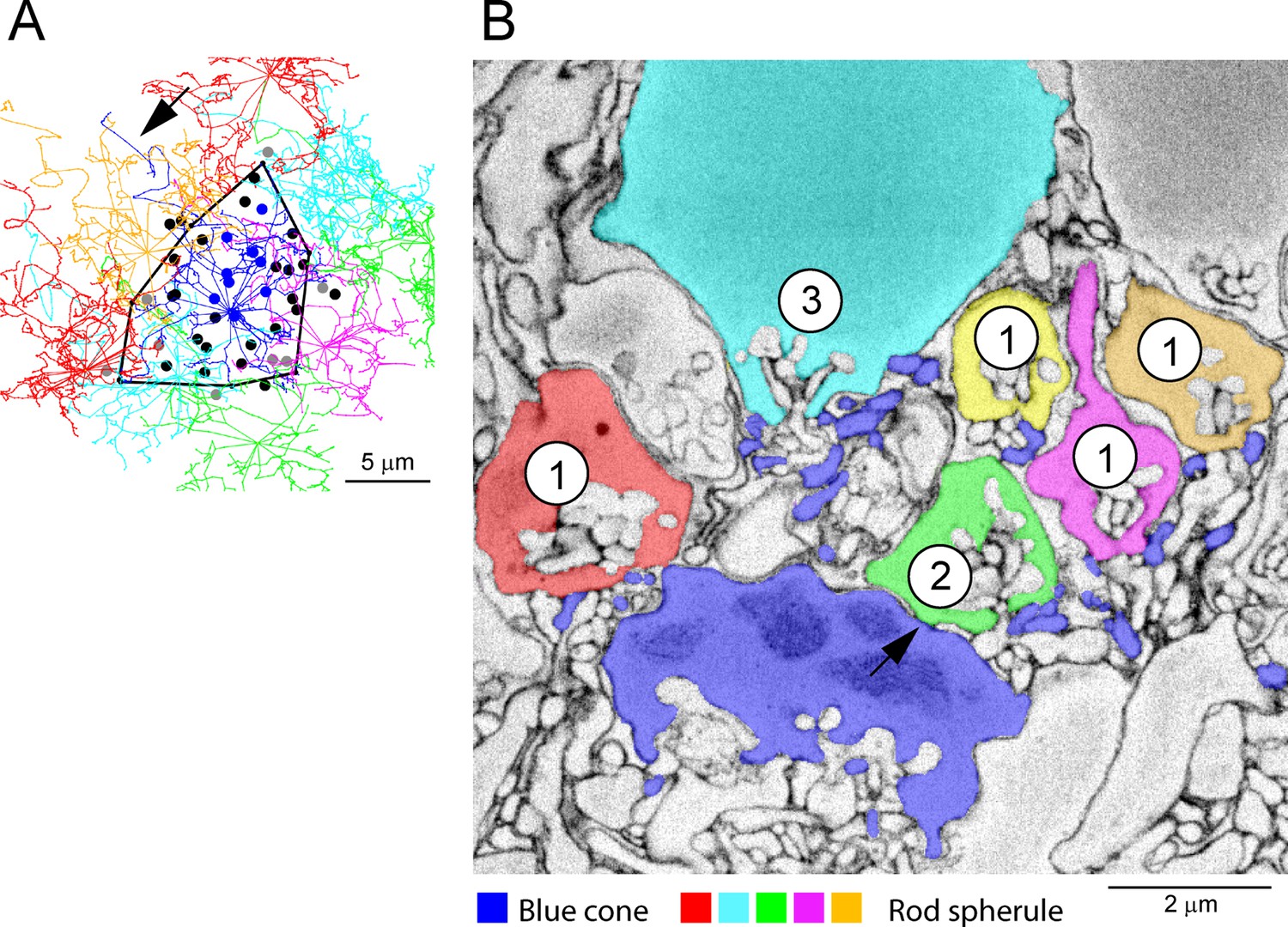
Blue cones, segmentation, e2006.
(A) Detail of cone pedicle skeletons from Figure 5 with the field of cone 2 outlined. This cone was identified as a blue cone by Behrens et al., 2016. Arrow shows axon. (B) Segmentation, e2006, blue cone pedicle (cone 2, dark blue) makes a variety of contacts with nearby rod spherules. (1) Telodendrial contacts close to the synaptic mouth of four rod spherules. (2) A roof contact, arrow, with a rod spherule (green). (3) Telodendrial contatcs with a low rod (cyan) in the lowest row of the outer nuclear layer (ONL). The contacts of blue cone pedicles are indistinguishable from green cones.
Figure 6—figure supplement 5
Blue cones e2006, 3D reconstruction.
(A) Reconstructed cone pedicles (cone 5, green, and cone 2, dark blue, arrowhead, identified as a blue cone by Behrens et al., 2016). Arrows indicate ascending axons among ghost cells of the outer nuclear layer (ONL) (gray). (B) The block of rods receiving contacts from three adjacent cone pedicles, cone 5 (green), cone 3 (cyan), and blue cone 2 (dark blue). (C) Rotated view showing the top surface of these three cone pedicles with contact pads in red, yellow, and orange. Arrows indicate ascending axons, arrowhead shows a ring-like structure of contacts. (D) Rotated view, bottom surface of the rod spherules with contact pads, arrowhead marks same ring of contacts, as in (C). (E) Detail showing several rod spherules receiving contacts from the blue cone 2 (orange) and cone 3 (yellow). Rod spherules receive contacts indiscriminately from blue and green cones or both simultaneously. Arrows mark cone axons.
Figure 6—video 1
3D reconstruction of a single cone (cone 5, green) with contact pads in red, then all rod spherules that were in contact with this cone.
Figure 6—video 2
A pair of reconstructed adjacent cone pedicles (cone 5, green, and cone 3, cyan).
A rotated view shows the contact pads from the top of the cone, then the contact pads from the bottom of the rod spherules, zooming in to show how a contact pad is close to the postsynaptic opening.
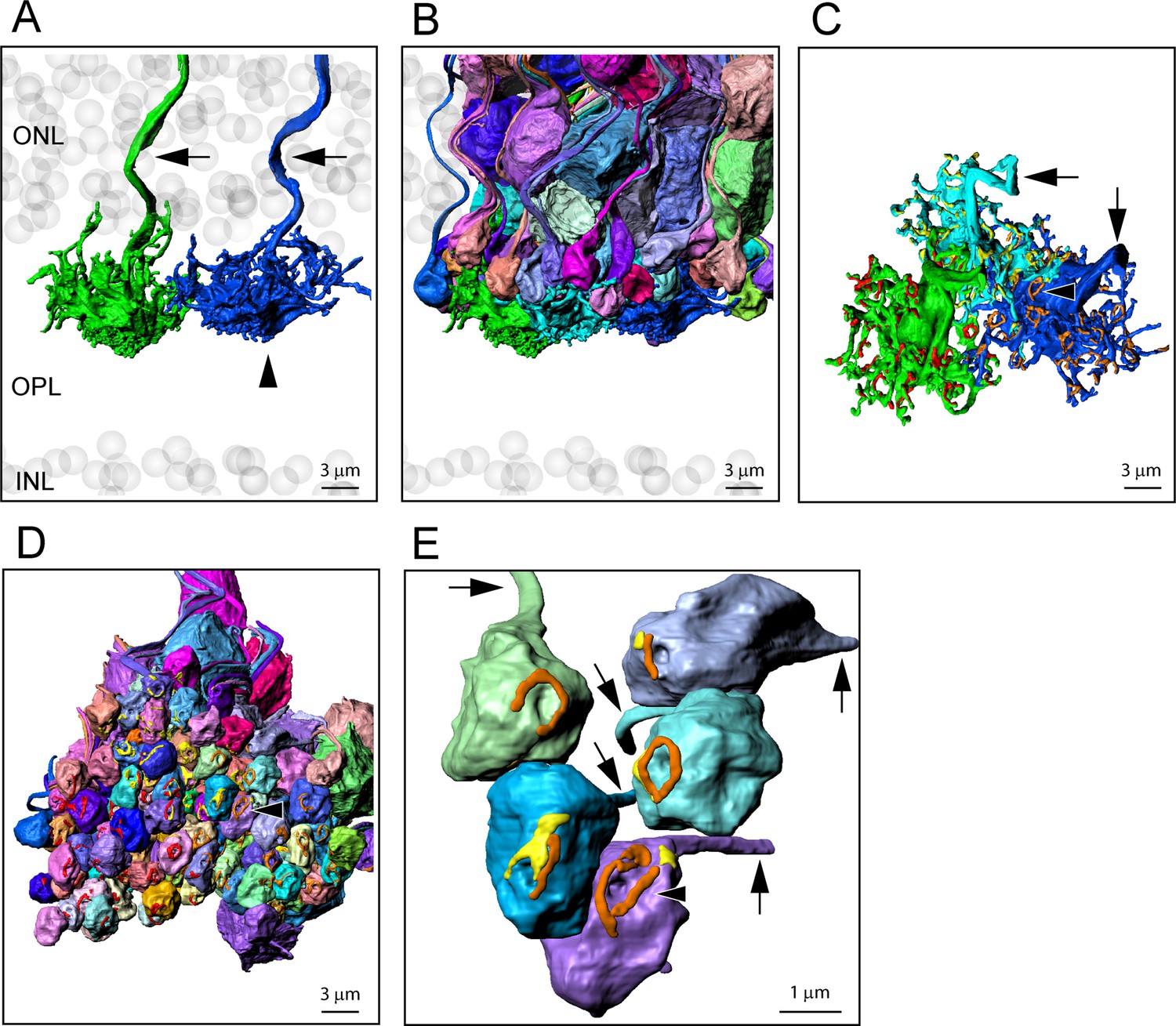
Figure 7 with 2 supplements

Segmentation and 3D reconstruction show gap junctions at rod/cone contacts.
(A) Serial blockface-scanning electron microscopy (SBF-SEM) dataset (eel001), a rod spherule (blue) nestled on the roof of a cone pedicle (green) with a densely stained gap junction contact (red arrow). (B) Magnified image of (A), detail showing an electron-dense gap junction (red arrow) with merged membranes. Note that there is clear separation except at this point. Postsynaptic inclusions indicate the gap junction is close to the synaptic opening of the rod spherule. (C) Focused ion beam-scanning electron microscopy (FIB-SEM): electron-dense gap junction staining at contact points (red arrow and arrowhead) between cone telodendria (green) and a rod spherule (blue). Inset: rotated en face view of one gap junction (red arrow) to measure length. (D) FIB-SEM: second example (red arrow) of an electron-dense gap junction at a cone contact (green) with a rod spherule (blue). Inset: en face view of the gap junction. Note that green cone telodendrial contact exceeds the gap junction staining. (E) FIB-SEM: overview of a rod spherule (blue) with a transparent reconstruction over the image planes in (F) and (G). Note the large mitochondrion towards the top of the rod spherule. (F) Image plane of the rod spherule (blue) through the synaptic opening with a small gap junction on each side (arrows) at a cone contact (green). (G) Image plane close to the base of the rod spherule (blue) reveals the two small gap junctions in (F) are part of a single large gap junction. There is a horseshoe-shaped gap junction (arrow) close to the synaptic opening where a cone telodendron (green) wraps around the base of the rod spherule. Large Cx36 horseshoe-shaped Cx36 clusters like this are easily observed by confocal microscopy. (H) FIB-SEM 3D reconstruction of the rod spherule (transparent blue) showing a single large gap junction (red, arrow) around the synaptic opening at the base. Postsynaptic inclusions are also rendered with two rod bipolar dendrites (gray and cyan) and two horizontal cell processes (green and purple). The synaptic ribbon is shown in yellow, partially obscured by the postsynaptic processes. Figure 7—video 1 shows this dataset.
Figure 7—figure supplement 1
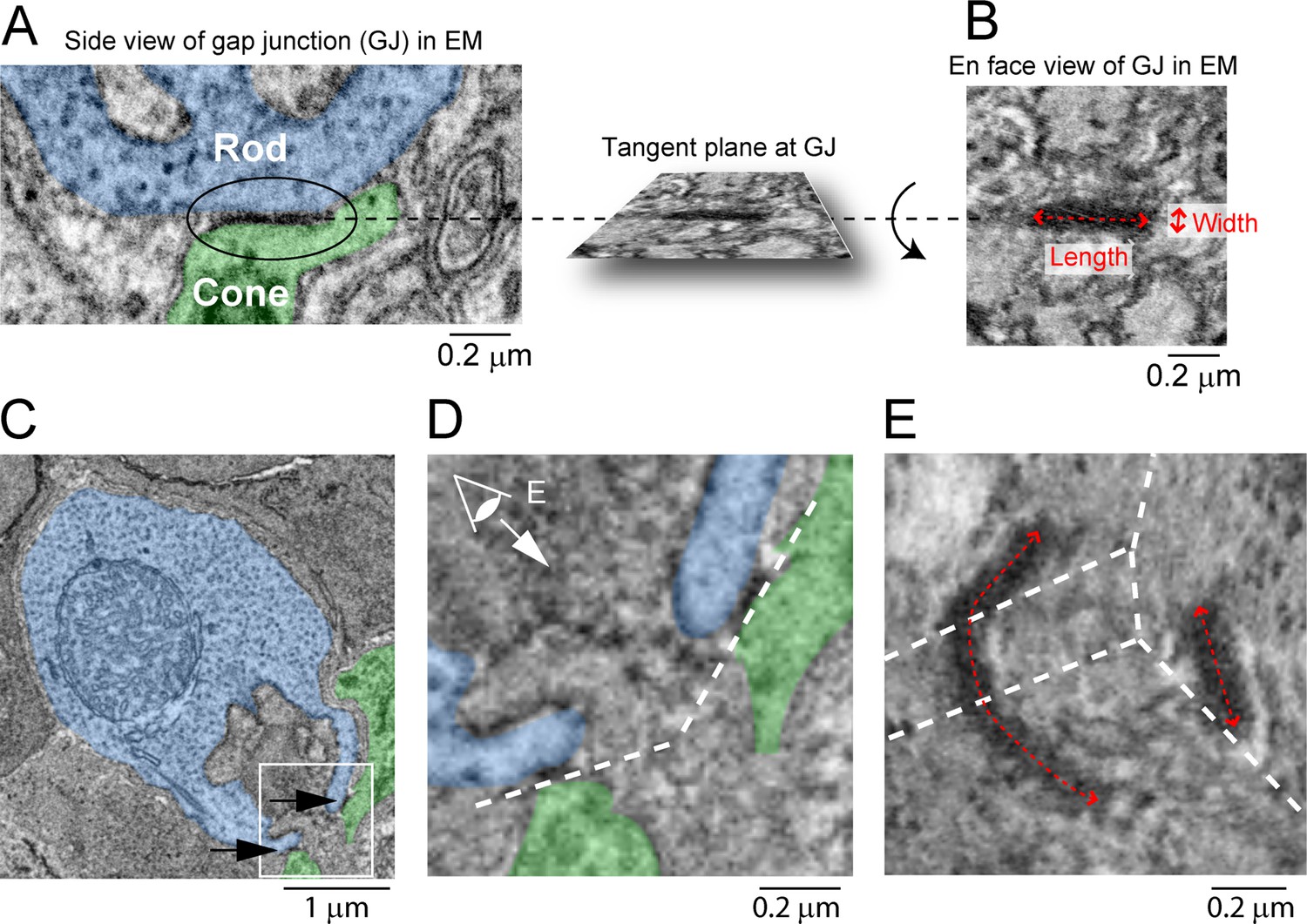
Measurement of gap junction (GJ) size in focused ion beam-scanning electron microscopy (FIB-SEM).
(A) Rod/cone contact in ellipse shows electron-dense staining of a GJ. (B) The tangent plane parallel to the cell membranes at the GJ (A) was acquired. This yields a belt-like structure. The center line in the longer dimension of the belt was measured as the length of the GJ. Width was measured as the shorter dimension. (C–E) Some electron-dense structures showed complicated shapes as in Figure 7H. Rod spherule in (C) has two GJs (arrows). (D) is enlarged picture of inset in (C), and dashed lines indicate tangent planes at GJs. To visualize one of the two GJs requires several planes as shown in (E). Dashed lines in (E) indicate intersections of the planes. Size of right GJ captured in one plane was measured as in (B). Length of left GJ was measured as summed length from three planes.
Figure 7—video 1
3D reconstruction showing a large horseshoe-shaped gap junction (red) around the base of a transparent rod spherule with postsynaptic processes also filled (from focused ion beam-scanning electron microscopy [FIB-SEM]).
Figure 8
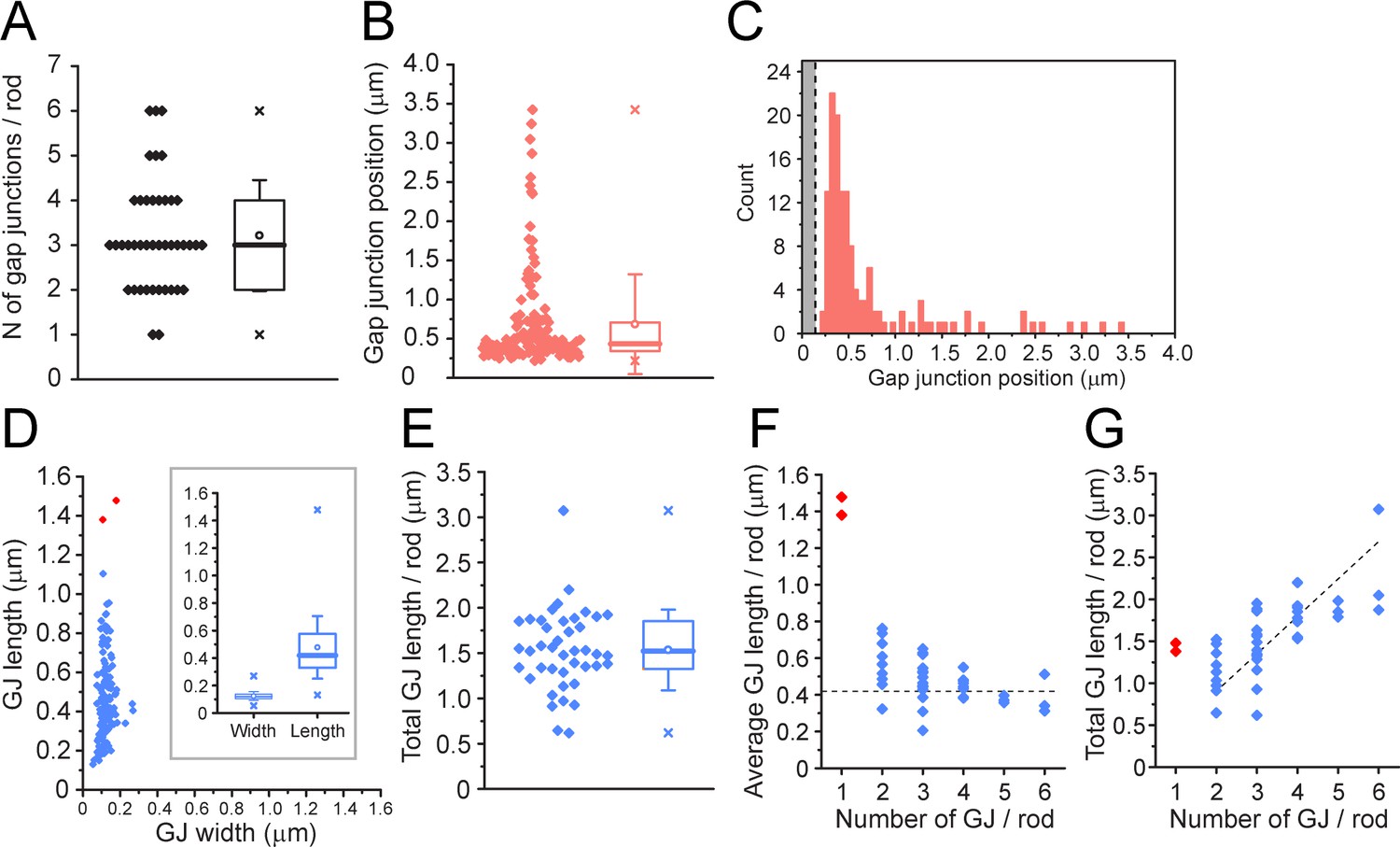
Quantitative analysis of 42 reconstructed rod spherules from focused ion beam-scanning electron microscopy (FIB-SEM).
(A) The number of gap junctions per rod spherule ranged from 1 to 6 (3.21 ± 1.23, mean ± SD, n = 42). Box shows quartiles, mean (circle), median (bold line), SD (whisker), min/max (x). (B) Gap junction distance from the rod spherule synaptic opening, skewed distribution, median, 0.435 μm. Box shows quartiles, mean (circle), median (bold line), SD (whisker), min/max (x). (C) Histogram plots of gap junction position, gray area shows radius of the synaptic opening (0.138 ± 0.121 μm, n = 42 rod spherules). (D) Gap junction length vs. width for 135 gap junctions from 42 rod spherules. Note restricted width compared to much greater variability in length, consistent with string-like structure. Box shows quartiles, mean (circle), median (bold line), SD (whisker), min/max (x) for width and length. Outliers in red are from rod spherules with a single large gap junction. (E) Total gap junction length per rod for 42 rod spherules. Box shows quartiles, mean (circle), median (bold line), SD (whisker), min/max (x). (F) Average gap junction length plotted as a function of the number of gap junctions per rod shows that if there is only one gap junction per rod spherule, it is a long one. The two longest gap junctions from (D) were both singles (red, same two as in D). These are easily observed when labeled for Cx36 using confocal microscopy (Figure 2—figure supplement 3; Jin et al., 2020). The dashed line is the median gap junction length (0.419 μm), and it runs through the data for multiple gap junctions per rod. In other words, each additional gap junction is approximately a standard size. (G) Total gap junction length per rod spherule as a function of the number of gap junctions per rod shows that the single gap junctions (red) are outliers with great length. Total gap junction length tends to rise with the number of gap junctions. The straight line of linear regression shows the effect of adding a standard mean gap junction length (0.44 μm) each time and runs through all the data except for the singles (red). Fitted line is y = 0.44x; (R2 = 0.33).
-
Figure 8—source data 1
Quantitative analysis of rod spherules from focused ion beam-scanning electron microscopy (FIB-SEM).
Source data for Figure 8A–G.
- https://cdn.elifesciences.org/articles/73039/elife-73039-fig8-data1-v3.xlsx
Figure 9
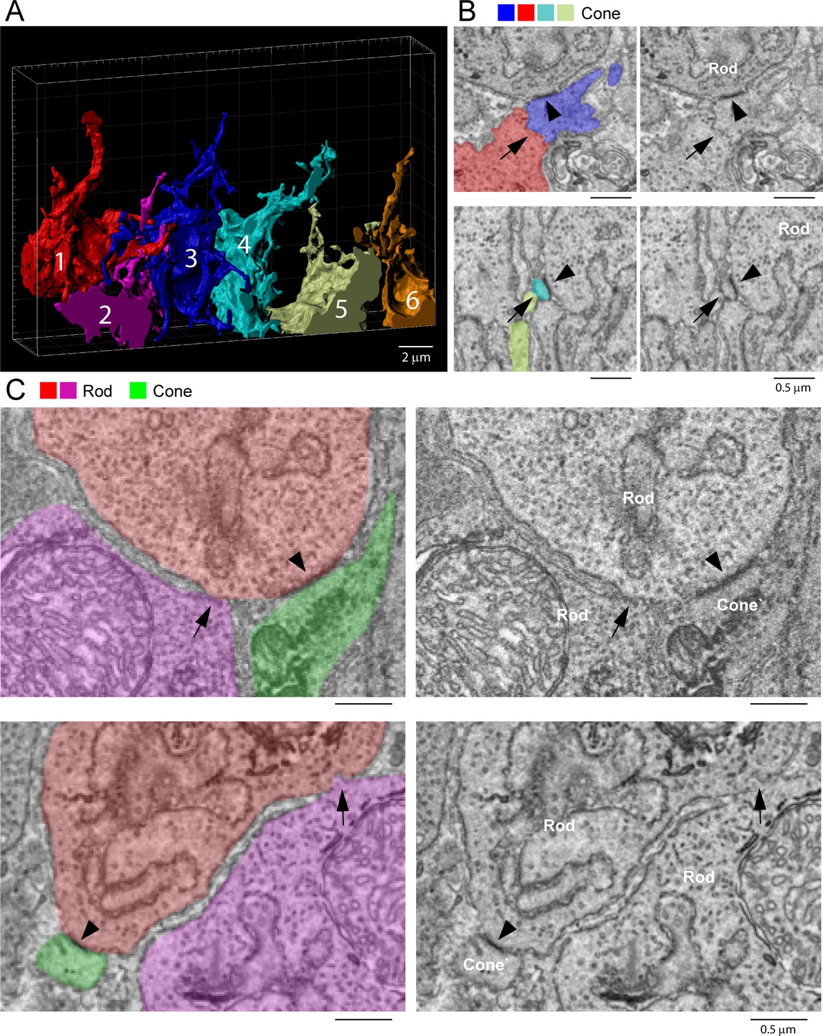
Rod/rod and cone/cone contacts do not appear as gap junctions, focused ion beam-scanning electron microscopy (FIB-SEM).
(A) Partial reconstruction of six cone pedicles from FIB-SEM. (B) Examples of cone/cone contacts (red/blue or yellow/cyan, arrows), which show no membrane density. These examples were selected because of the nearby rod/cone contacts (arrowheads), which show prominent dense staining at their contact points, consistent with the presence of a gap junction. (C) Rod/rod contacts (red/magenta, arrows) show no membrane specialization compared to nearby rod/cone gap junctions (red/green, arrowheads).
Figure 10
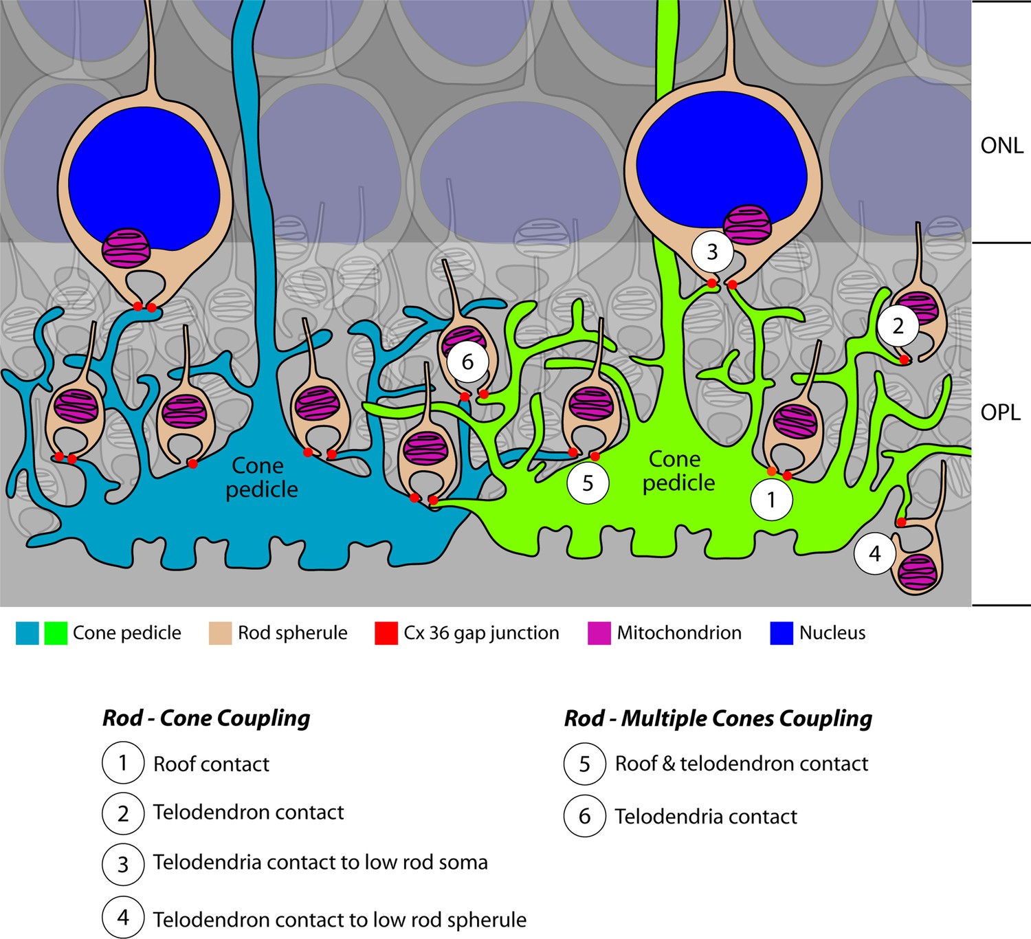
Cartoon summary of rod/cone gap junctions in the mouse retina.
A cartoon showing the variety of Cx36 rod/cone gap junctions, including cone telodendrial contacts, cone pedicle roof contacts, and inverted rod spherules. The lowest row of rod cell bodies in the outer nuclear layer (ONL) do not have axons or rod spherules but still have Cx36 gap junctions with cone telodendria, which reach the upper margin of the outer plexiform layer (OPL). All these structural variants were also found with blue cone pedicles, indicating that there was no color specificity in rod/cone coupling. Most rod spherules have gap junction contacts with more than one cone. All rod spherules, with very few exceptions (such as areas of low cone density), make gap junctions with nearby cone pedicles. In contrast to the numerous rod/cone gap junctions, we could not detect rod/rod or cone/cone gap junctions in these experiments.
Tables
Table 1
Antibodies.
| Antibody | Source | Catalog # | Species | Dilution | Notes |
|---|---|---|---|---|---|
| Cone arrestin | Millipore | AB15282 | Rabbit | 1:1000 | Labels cones, including pedicle |
| Cx36 | Millipore | MAB3045 | Mouse | 1:1000 | Cx36 gap junctions |
| vGlut1 | Synaptic Systems | 135304 | Guinea pig | 1:3000 | Labels PR terminals, especially rod spherules |
| Blue cone opsin | Millipore | AB5407 | Rabbit | 1:1000 | Blue cone outer segments |
| Ribeye/CtBP2 | BD Transduction | 612044 | Mouse | 1:500 | Synaptic ribbon marker |
| TOMM20 | Santa Cruz | SC-11415 | Rabbit | 1:1000 | Mitochondrial marker |
| mGluR6 | Generous gift from Kiril Martemyanov | Sheep | 1:1000 | mGluR6 receptors of ON bipolar cells and rod bipolar cells | |
| PMCA | Santa Cruz Biotechnology | sc-28765 | Rabbit | 1:200 | Labels rod spherule plasma membrane |
Appendix 2—table 1
Analysis of photoreceptors by serial blockface-scanning electron microscopy (SBF-SEM) from e2006.
| All cones | Central cones | p-Value | |
|---|---|---|---|
| N of cones | 29 | 13 | |
| N of rods | 811 | 361 | |
| Rods/cone | 28.0 | 27.8 | |
| Convergence | |||
| Mean ± SD | 43.0 ± 5.40 | 41.7 ± 4.19 | 0.40 |
| Median (Q1–Q3) | 43 (39–46) | 43 (38–45) | |
| Divergence | 1.54 ± 0.628 | 1.89 ± 0.639 | 2.5 × 10⁻¹⁷ |
| Conv./div. | 28.0 | 22.1 | |
| Cone coverage area* | |||
| Mean ± SD | 104 ± 20.2 | 102 ± 14.5 | |
| Median (Q1–Q3) | 100 (86.7–117) | 99.9 (93.0–111) | |
| Area covered by cones* | 1920 | 890 | |
| Cone density† | 0.0151 | 0.0146 | |
| Coverage | 1.56 | 1.49 | |
| N of shared rods | |||
| Mean ± SD | 6.23 ± 4.67 (N = 79) | 5.85 ± 4.42 (N = 61) | 0.63 |
| Median (Q1–Q3) | 4 (2–8) | 5 (2–9) |
-
Unit is *(μm2) and †(/μm2).
Appendix 2—table 2
Comparison of blue and green cones.
| Blue cones | Green cones | p-Value | |
|---|---|---|---|
| N of cones | 5 | 31 | |
| Convergence | |||
| Mean ± SD | 39.8 ± 5.11 | 43.0 ± 6.86 | 0.31 |
| Median (Q1–Q3) | 39 (39–41) | 43 (39–46) | |
| Cone coverage area* | |||
| Mean ± SD | 85.1 ± 18.6 | 104 ± 21.8 | 0.081 |
| Median (Q1–Q3) | 83.4 (76.4–98.0) | 105 (84.8–120) | |
| N of shared rods | |||
| Mean ± SD | 6.56 ± 6.34 (N = 16) | 6.26 ± 4.14 (N = 69) | 0.86 |
| Median (Q1–Q3) | 6 (3–9) | 3.5 (2–10.8) |
-
Unit is *(μm2).
Appendix 2—table 3
Focused ion beam-scanning electron microscopy (FIB-SEM) analysis.
| N of rods | 42 |
| N of gap junction/rod | |
| Mean ± SD | 3.21 ± 1.23 |
| Median (Q1–Q3) | 3 (2–4) |
| Gap junction position* | |
| Mean ± SD | 0.686 ± 0.635 |
| Median (Q1–Q3) | 0.435 (0.345–0.703) |
| Synaptic mouth radius* | 0.138 ± 0.121 |
| Gap junction width* | |
| Mean ± SD | 0.123 ± 0.0320 |
| Median (Q1–Q3) | 0.120 (0.103–0.138) |
| Gap junction length* | |
| Mean ± SD | 0.477 ± 0.227 |
| Median (Q1–Q3) | 0.419 (0.332–0.568) |
| Total gap junction length/rod* | |
| Mean ± SD | 1.53 ± 0.439 |
| Median (Q1–Q3) | 1.52 (1.33–1.85) |
-
Unit is *(μm).
Additional files
Download links
A two-part list of links to download the article, or parts of the article, in various formats.
Downloads (link to download the article as PDF)
Open citations (links to open the citations from this article in various online reference manager services)
Cite this article (links to download the citations from this article in formats compatible with various reference manager tools)
Analysis of rod/cone gap junctions from the reconstruction of mouse photoreceptor terminals
eLife 11:e73039.
https://doi.org/10.7554/eLife.73039


