Strategy-dependent effects of working-memory limitations on human perceptual decision-making
- Department of Neuroscience, University of Pennsylvania, United States
- Department of Mathematics, University of Houston, United States
- Department of Biology and Biochemistry, University of Houston, United States
- Department of Applied Mathematics, University of Colorado Boulder, United States
- Institute of Cognitive Science, University of Colorado Boulder, United States
Figures
Figure 1
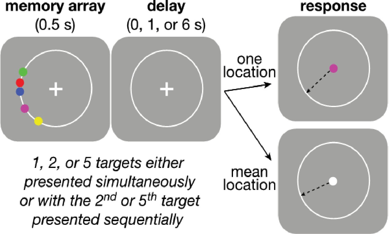
Behavioral task.
Participants were asked to maintain visual fixation on the center cross while an array of colored disks was presented for 0.5 s, followed by a variable delay and finally the presentation of a visual cue whose color was either: (1) the same as one of the disks, indicating that the participant should use the mouse to mark the remembered location of that disk (‘Perceptual’ trial) or (2) white, indicating that the participant should mark the mean angle of the array (‘Computed’ trial). Perceptual and Computed trials were presented in separate, signaled blocks. On Perceptual trials, participants did not know in advance which disk would be probed on any given trial. The number of disks and length of the delay period were varied randomly within each block. Blocks were also defined by the temporal presentation of the disks. In ‘Simultaneous’ blocks, all disks were presented at once, whereas in ‘Sequential’ blocks, the final disk (always the most counter-clockwise of all disks presented on that trial) was presented midway through the variable delay. In all blocks, the disks always had the same clockwise ordering by color, as depicted in the ‘memory array’ graphic above, to minimize binding errors between color and location in the Perceived blocks.
Figure 2 with 1 supplement
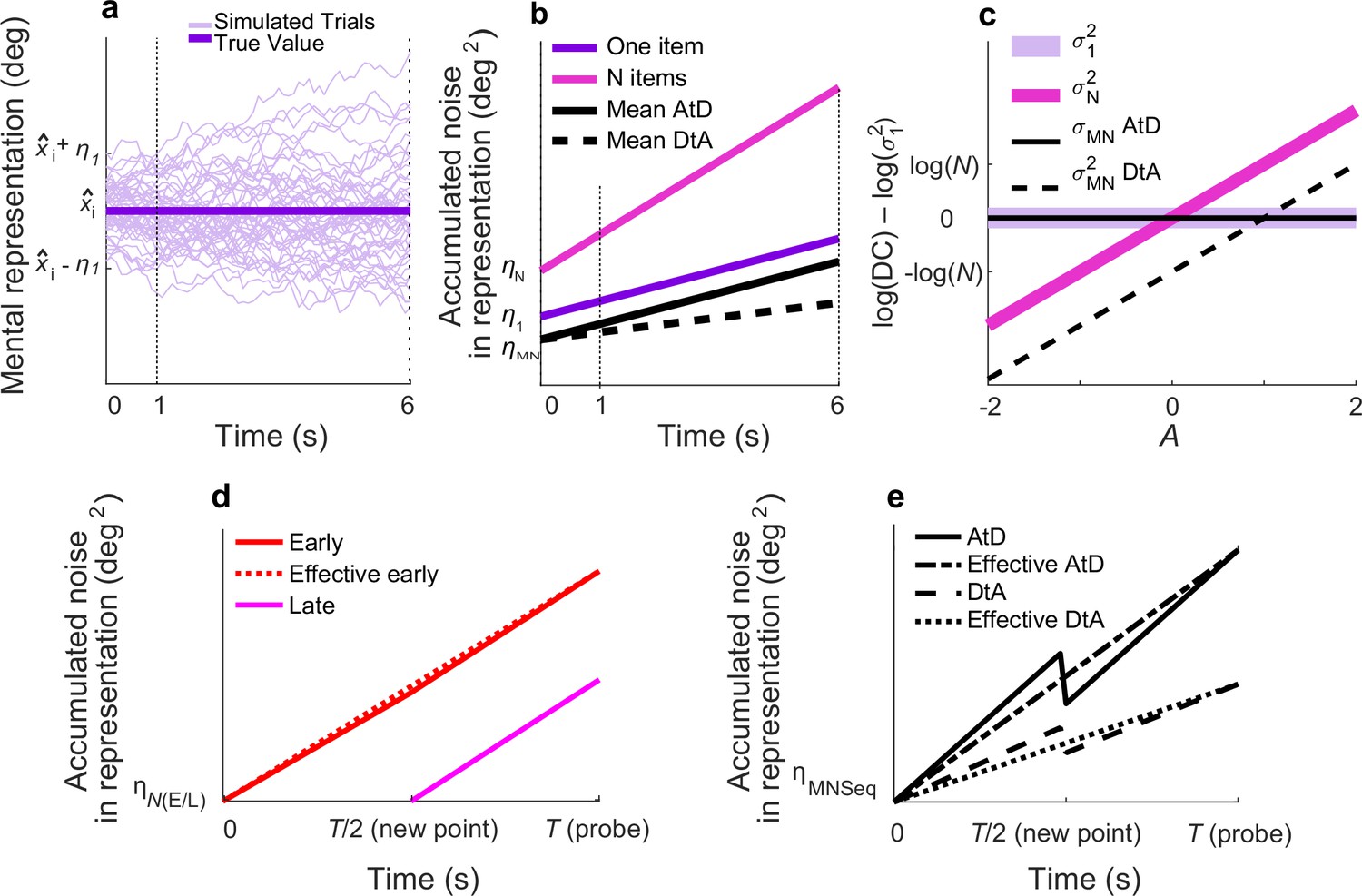
Diffusion model and predictions for different strategies.
(a) Fifty simulated trials of the representation of a single memorandum, x̂I, corrupted by a static noise term representing sensory and motor noise (η1) and time-dependent noise (increasing variance corresponding to decreasing memory precision) modeled as Brownian diffusion. At time t, the report for one item, rt,1, is the location of the particle. (b) Linear accumulation of noise (variance) for single or multiple Perceived items (colors, as indicated) or Computed mean values using two different strategies (solid vs. dashed black lines, as indicated). Memory representations of N=1, 2, or 5 items have initial, additive error ηN and diffuse over time with diffusion constant σN2; thus, variance at time t=ηN+t*σN2. For the Average-then-Diffuse (AtD) model, the average is calculated immediately and stored as a single value. Thus, the diffusion constant of a Computed mean of N items is the same as for one item (σMN2=σ12; parallel purple and black lines), although η1 and ηMN may not be equal. For the Diffuse-then-Average (DtA) model, all items are stored until the probe time. Thus, the effective σMN2 is 1/Nth of σN2. (c) Relationship between A and log differences of diffusion constants for various set sizes and models. σ12 is independent from A and equal to σMN2 under AtD. σN2 is linear with A in log space with respect to (σ12) because log(σN2)–log(σ12)=A*log(N). σMN2 is linear with A. DC=Diffusion Constant. (d) Accumulation of noise for Perceived items presented sequentially. When the new (Late) point is added at time T/2, the diffusion constant for previously presented items (Early) changes slightly because of the increased load. Early and Late items for set size N have encoding noise ηNE and ηNL, respectively, represented by η(E/L). The ‘effective Early’ trace shows the net gain in variance over time that would be expected when sampling the error only at a single time T, as we did. (e) Accumulation of noise for Computed items in the Sequential condition for both models. The encoding noise for the mean of N items is represented by ηMNSeq. At time=T/2, the final point is averaged, causing a change in the diffusion constant. The ‘effective’ lines represent the measured change in variance over time one would measure when recording only at T. Here N=5, A=0.5.
Figure 2—figure supplement 1

Identifiability of AtD and DtA models as a function of the A parameters.
(a) Simulations from set size 2. (b) Simulations from set size 5. For each participant, 1000 task simulations were generated using their best-fit model and parameters, and then each simulation was refit to both the AtD and DtA models and the fits compared via log-likelihoods. The ordinate indicates the percentage of those simulations for which the true (simulate) generative model was identified correctly. In general, identifiability was higher when A was not near 1, as expected, and for set size 5 versus 2. AtD, Average-then-Diffuse; DtA, Diffuse-then-Average.
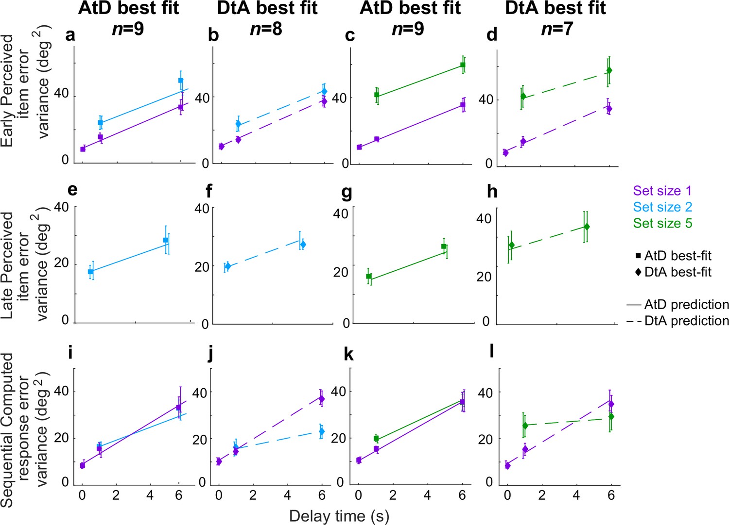
Figure 3 with 3 supplements
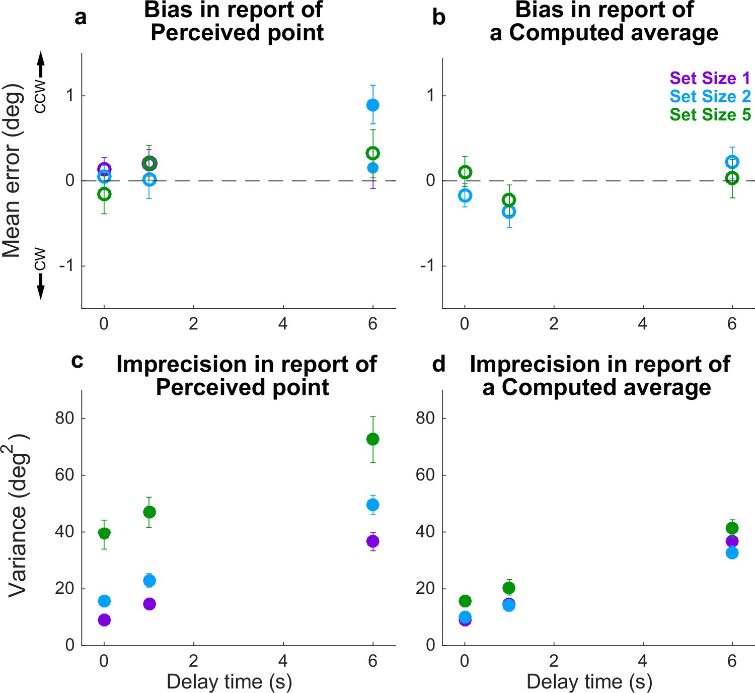
Behavioral summary for the Simultaneous condition.
(a) Mean Perceptual error for different set sizes (colors, as indicated) and delay times (abscissa). Filled points indicate two-tailed t-test for H0: mean=0, p<0.05. (b) Mean Computed (inferred mean) error for different set sizes (colors, as indicated) and delay times (abscissa). For all tests, mean error was not significantly different from 0 (p>0.05; open circles). (c) Variance in Perceptual errors, plotted as in (a). (d) Variance in Computed (mean) errors, plotted as in (b). In each panel, points and error bars are mean ± SEM across participants.
Figure 3—figure supplement 1
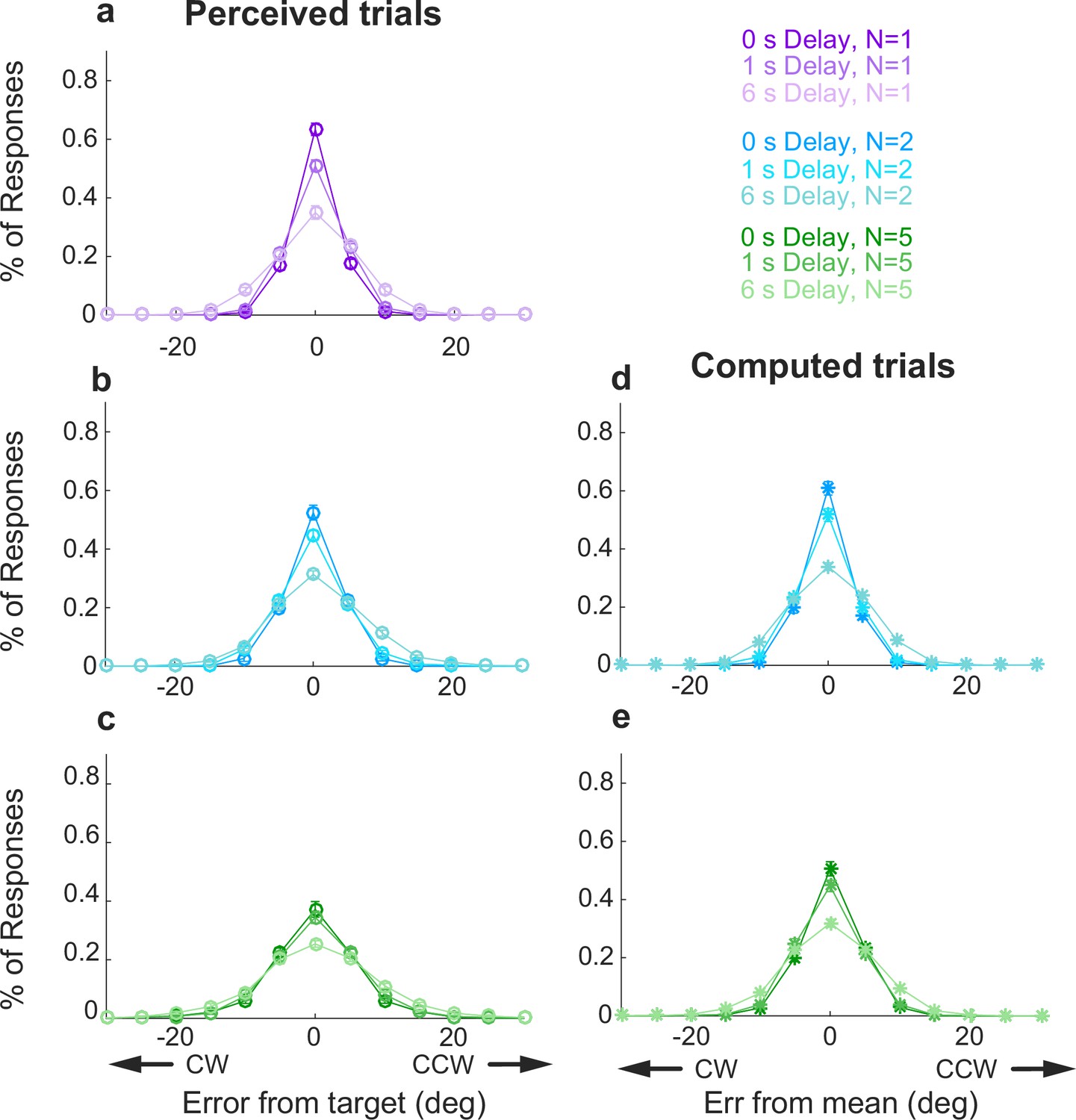
Full error distributions in Simultaneous conditions.
Each panel shows a histogram of mean error for different delays (colors, as indicated). Perceived trials: (a) set size=1; (b) set size=2; (c) set size=5. Computed trials: (d) set size=2; (e) set size=5. In each panel, points and error bars are mean ± SEM across all participants. Note that in all cases, 95% of the distributions fall between –30° and 30°, justifying our exclusion of larger errors as off-target responses.
Figure 3—figure supplement 2
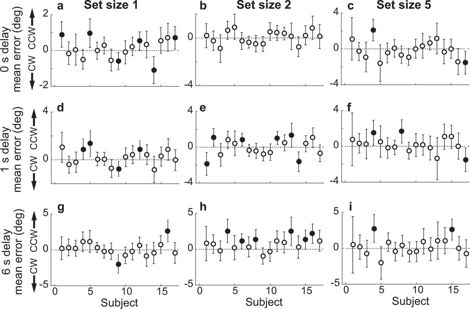
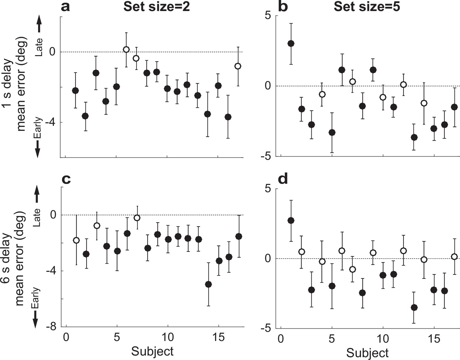
Participant-wise mean response error in the Simultaneous Perceived condition.
(a) Delay=0 s, set size=1. (b) Delay=0, set size=2. (c) Delay=0 s, set size=5. (d–f) Same as in (a–c), but for delay of 1 s. (g–i) Same as in (a–c), but for delay of 6 s. In all panels, error bars are ±95% confidence intervals (CIs). Filled points indicate that 0 is not included in the CI, that is, there was a bias in the given participant’s errors.
Figure 3—figure supplement 3
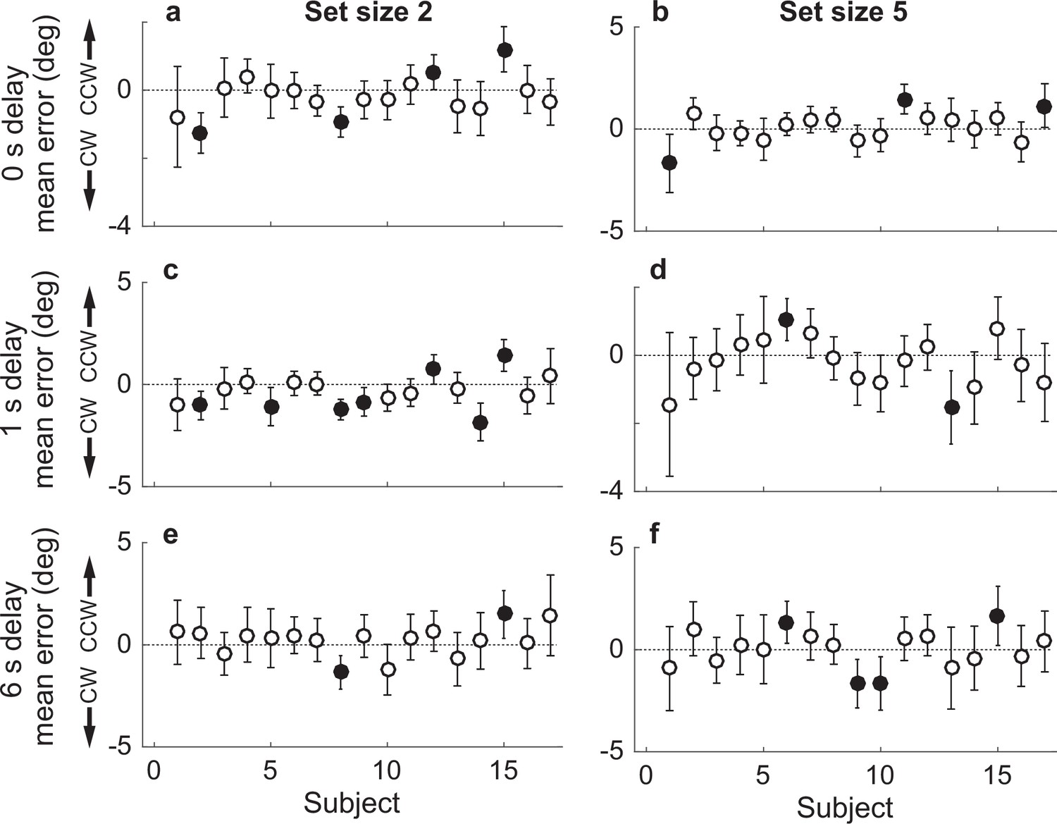
Participant-wise mean error in the Simultaneous Computed condition.
(a) Delay=0 s, set size=2. (b) Delay of 0, set size=5. (c, d) Same as in (a, b), but for delay of 1 s. (e, f) Same as in (a, b), but for delay of 6 s. In all panels, error bars are ±95% confidence intervals (CIs). Filled points indicate that 0 is not included in the CI, that is, there was a bias in the given participant’s errors.
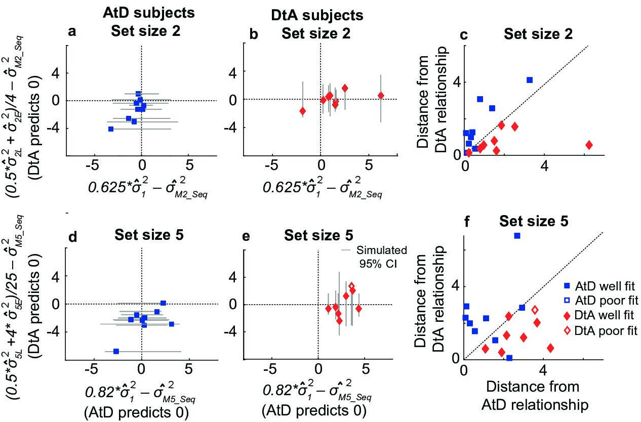
Figure 4 with 1 supplement

Comparisons of empirical and model-based diffusion constant relationships for the Simultaneous condition.
In (a, b, d, e), the abscissa shows the difference between: (1) empirical estimates of the diffusion constant for a Computed value measured by fitting a line to measured variance as a function of delay time for set size 2 (M22, a, b) or 5 (M52, d, e), and (2) the empirical estimates of the diffusion constant for a single Perceived value (12). The AtD model predicts a difference of 0. The ordinate shows the difference between: (1) the empirical estimate of Computed diffusion constants M22 or M52, and (2) the empirical estimates of the diffusion constant for multiple Perceived values (22 or 52) divided by the number of items. The DtA model predicts a difference of 0. Each point was obtained using data from individual participants, separated by whether they were best fit by the AtD (a, b) or DtA (d, e) model for the given set-size condition. Lines represent 95% confidence intervals (CIs) computed by simulating data using the best-fit parameters for the given fit and repeating the empirical estimate comparison procedure. Closed symbols indicate participants who fell within the 95% CI for their best-fit model. (e, f) Distance of each participant’s empirically estimated diffusion constant relationships from those predicted by AtD or DtA (i.e., distances from the x=0 and y=0 lines, respectively, in (a, b, d, e)), for set sizes 2 (c) and 5 (f).
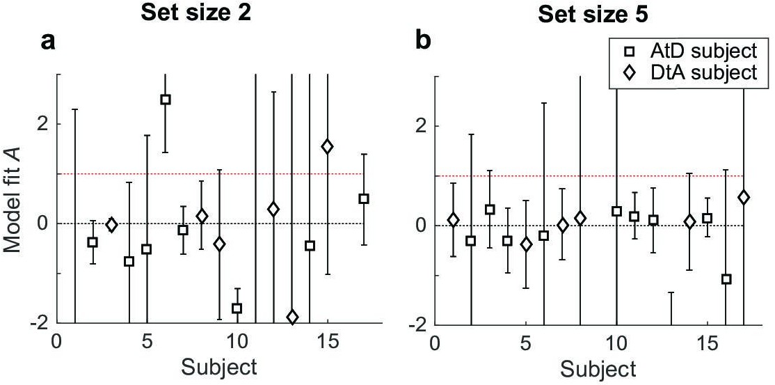
Figure 4—figure supplement 1
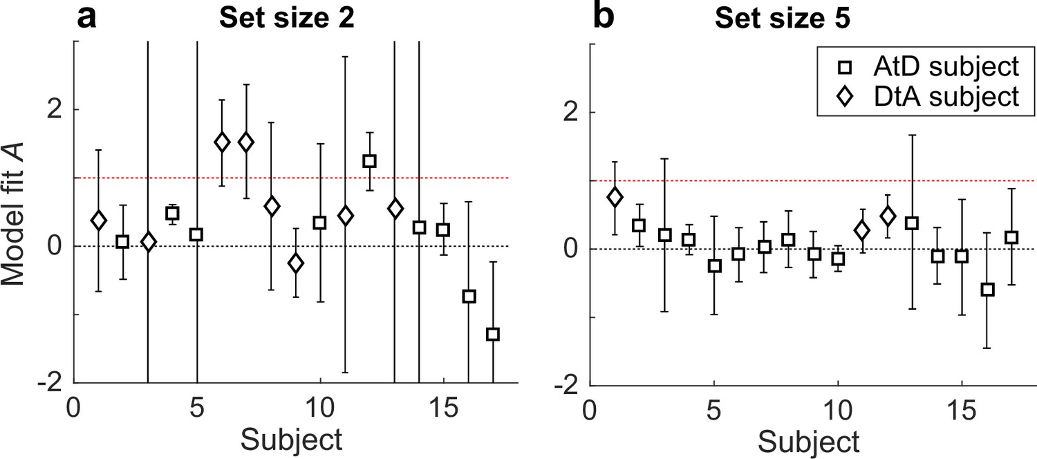
Participant-specific estimates of A from the Simultaneous condition for set sizes 2 (a) and 5 (b).
Symbols indicate best-fitting model (AtD or DtA), as indicated. In all panels, error bars are ±95% confidence intervals based on the Hessian computed during model fitting. Note that A=0 implies no difference between the diffusion constant for a single and N items, whereas A=1 implies that the variance and diffusion constant relationship predictions of the AtD and DtA models are equal and thus the models cannot be distinguished from each other. AtD, Average-then-Diffuse; DtA, Diffuse-then-Average.
Figure 5

Comparison of model prediction to participant data for the Simultaneous condition.
Each panel shows the empirical variance of participant errors (points and error bars are mean ± SEM data across participants) and model predictions (lines, based on the mean best-fitting parameters across participants for the given model) for the participants’ best fit by the given model (AtD or DtA) for the given condition, as labeled above each column. (a–d) Perceived blocks. (e–h) Computed blocks. AtD, Average-then-Diffuse; DtA, Diffuse-then-Average.
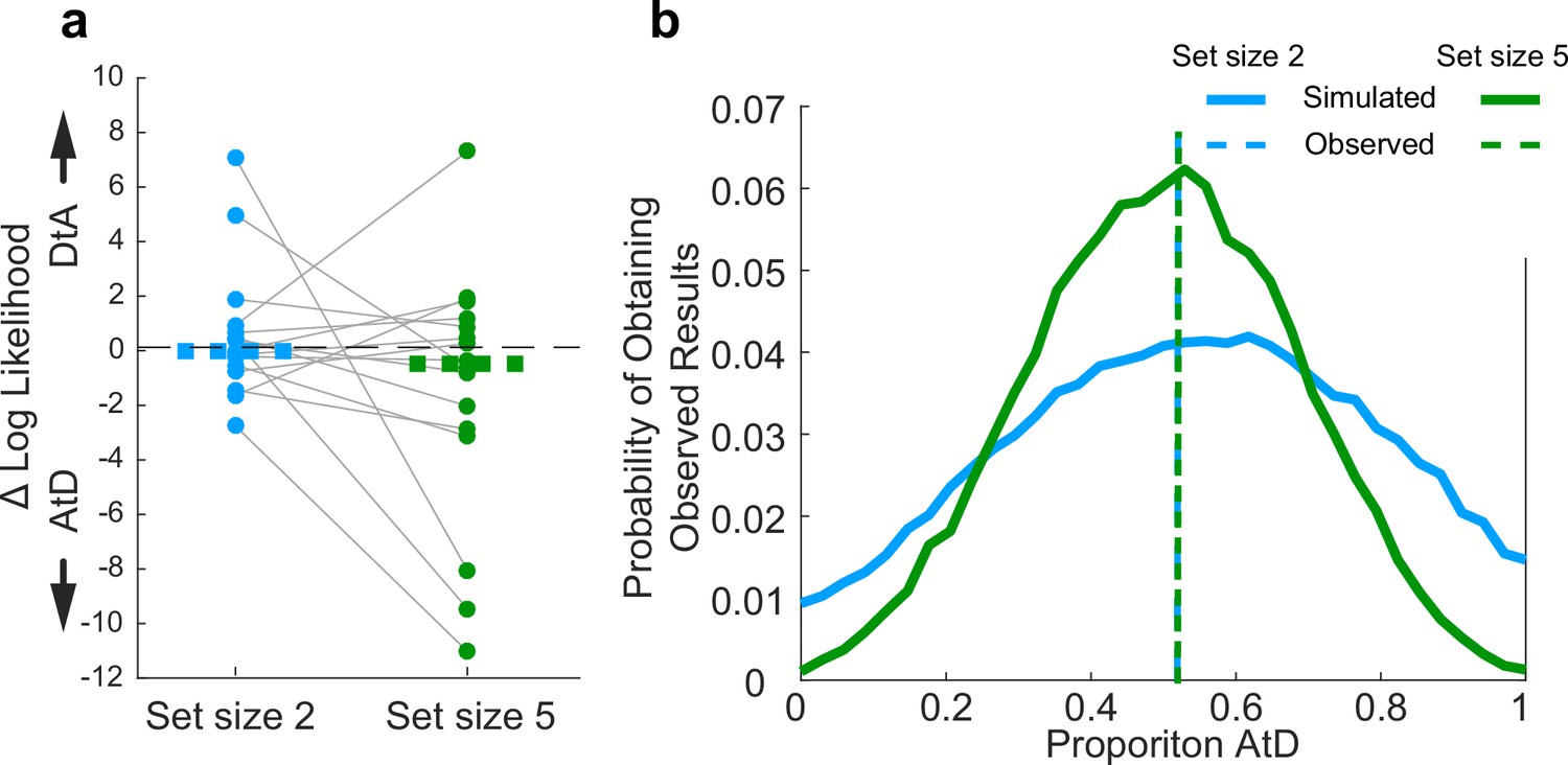
Figure 6 with 1 supplement
Strategy use prevalence in the population.
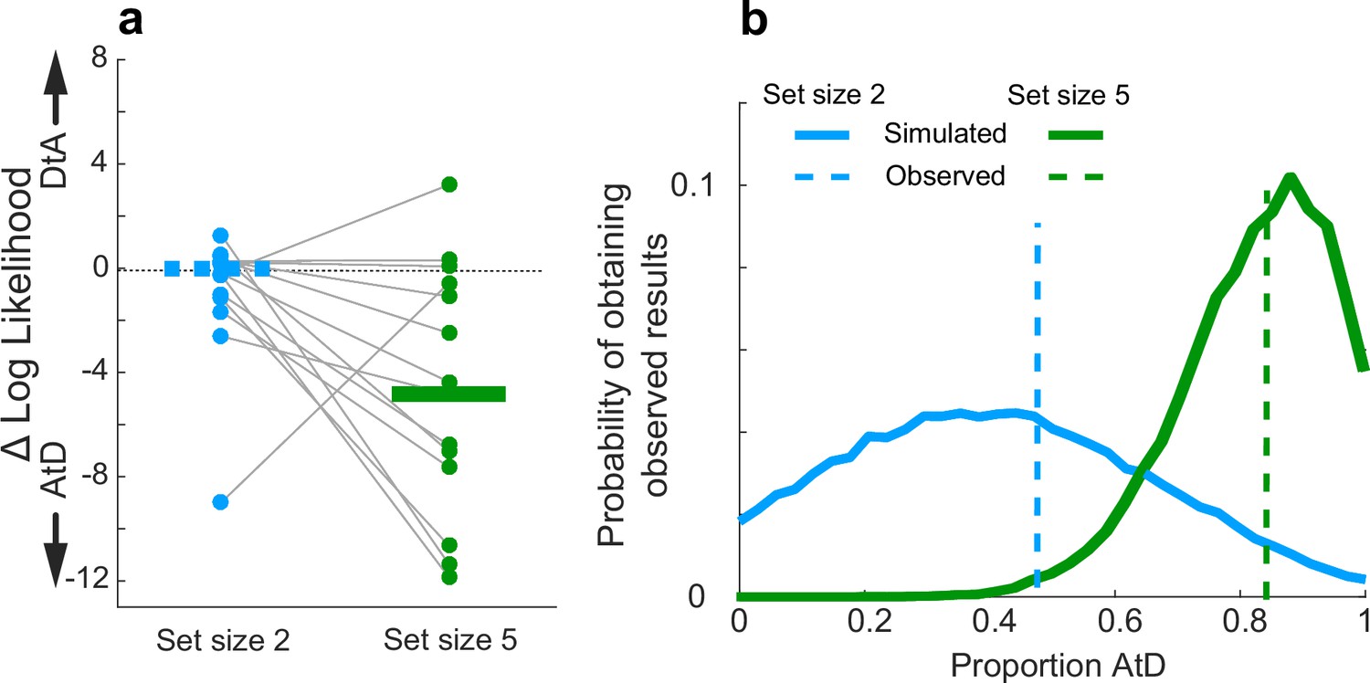
(a) Difference in log-likelihood between AtD and DtA fits for the Simultaneous condition. Each point represents the difference in fit log-likelihoods for one participant; horizontal bars are medians (solid bar for set size 5 indicates two-sided Wilcoxon signed-rank test for H0: median=0, p=0.0027). Positive values favor DtA, whereas negative favor AtD. Gray lines connect data generated by the same participant. Only participants whose data were well matched to one of the two models (i.e., within the 95% confidence intervals depicted in Figure 4) were included. (b) Probability of obtaining the proportion of participants’ best fit by each model given average model identifiability of participant parameters. Probability of the results at set size 5 skew toward a higher proportion of AtD users compared to set size 2. AtD, Average-then-Diffuse; DtA, Diffuse-then-Average.
Figure 6—figure supplement 1
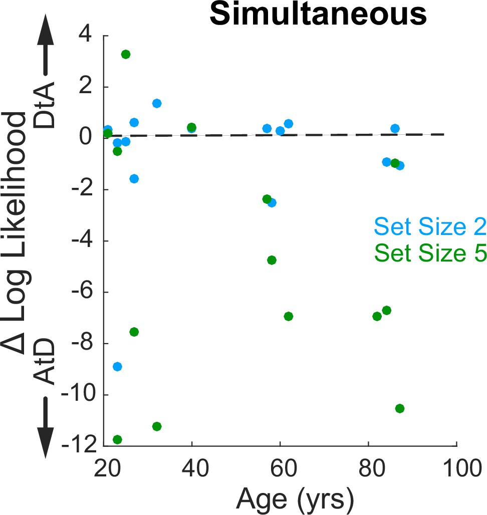
Relationship between log-likelihood difference for the two strategies and age for the Simultaneous condition.
Log-likelihood comparison for AtD and DtA (negative favors AtD) for set sizes 2 and 5 is not dependent upon age (correlation, ps>0.20 computed separately for each set size). AtD, Average-then-Diffuse; DtA, Diffuse-then-Average.
Figure 7 with 3 supplements
Behavioral summary for the Sequential condition.
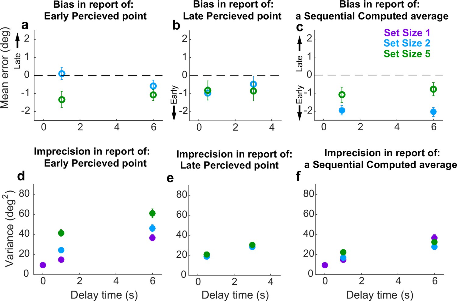
(a) Mean error for initially presented (Early) Perceptual items for different set sizes (colors, as indicated) and delay time (abscissa). (b) Mean error for midway presented (Late) Perceptual items for different set sizes (colors, as indicated) and delay time (abscissa). (c) Mean Computed (inferred mean) error for different set sizes (colors, as indicated) and delay time (abscissa). Filled points in (a–c) indicate two-tailed student t-test for H0: mean=0, p<0.05. (d) Variance in Early Perceptual errors plotted as in (a). (e) Variance in Late Perceptual errors, plotted as in (b). (f) Variance in Computed (mean) errors, plotted as in (c). In each panel, points and error bars are mean ± SEM across participants.
Figure 7—figure supplement 1

Full error distributions in Sequential conditions.
Each panel shows a histogram of mean error for different delays (colors, as indicated). Perceived Early: (a) set size=2; (b) set size=5. Perceived Late: (c) set size=2; (d) set size=5. Computed trials: (e) set size=2; (f) set size=5. In each panel, points and error bars are mean ± SEM across all participants. Note that in all cases, 95% of the distributions fall between –30° and 30°, justifying our exclusion of larger errors as off-target responses.
Figure 7—figure supplement 2
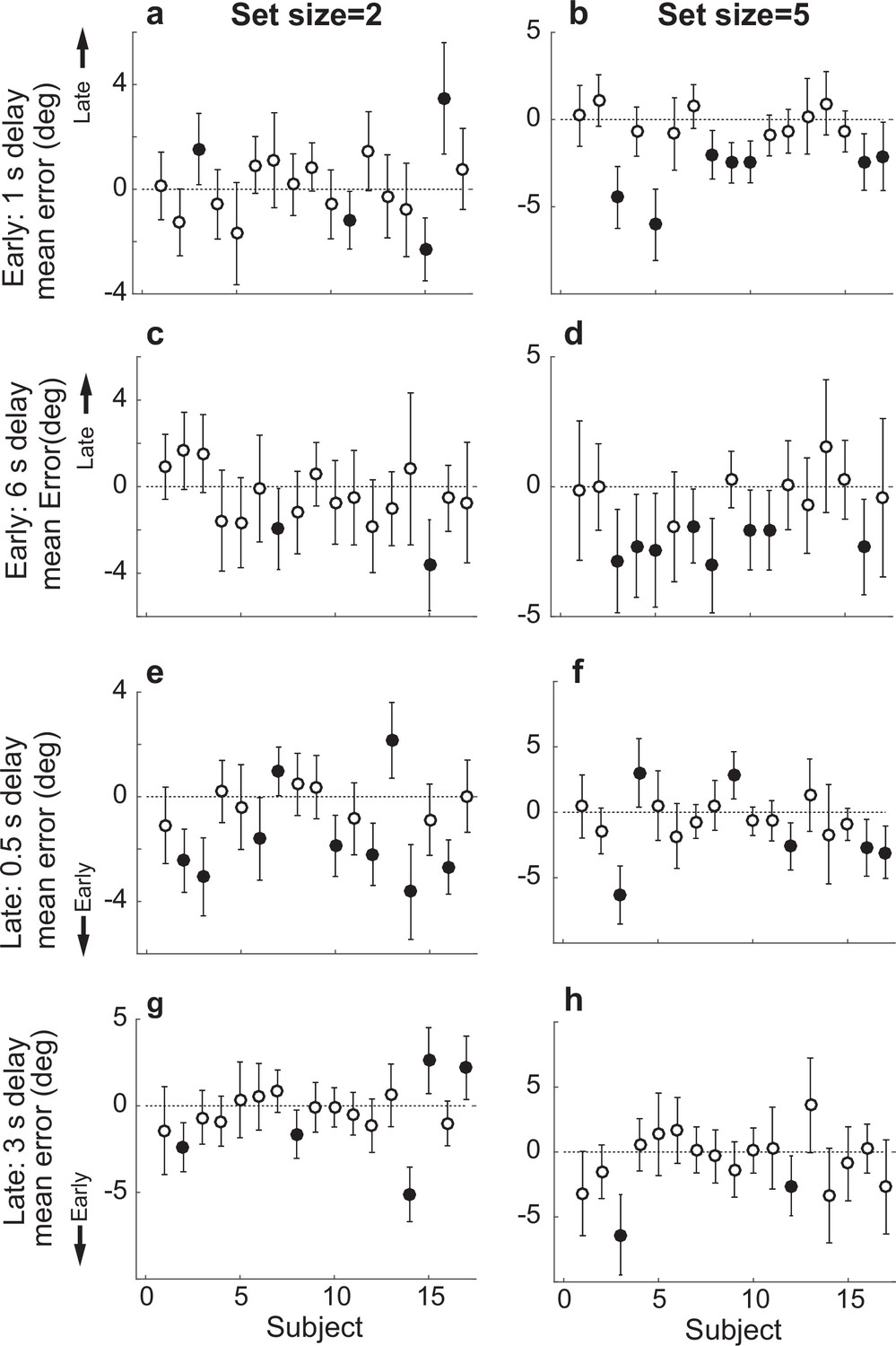
Participant-wise mean error in the Sequential Perceived condition.
(a) Delay=1 s, set size=2 for Early samples. (b) Delay=1, set size=5 for Early samples. (c, d) Same as in (a, b), but for delay of 6 s. (e) Delay=0.5 s, set size=2 for Late samples. (f) Delay=0.5 s, set size=5 for Late samples. (g, h) Same as in (e, f), but for delay of 3 s. In all panels, errorbars are ±95% confidence intervals (CIs). Filled points indicate that 0 is not included in the CI, that is, there was a bias in the given participant’s errors.
Figure 7—figure supplement 3
Participant-wise mean error in the Sequential Computed condition.
(a) Delay=1 s, set size=2. (b) Delay=1, set size=5. (c, d) Same as in (a, b), but for delay of 6 s. In all panels, error bars are ±95% confidence intervals (CIs). Filled points indicate that 0 is not included in the CI, that is, there was a bias in the given participant’s errors (which in this case tended to be toward the mean computed from the early items).
Figure 8 with 1 supplement
Comparisons of empirical and model-based diffusion constants.
In (a, b, d, e), the abscissa shows the difference between: (1) empirical estimates of the diffusion constant for a Computed value measured by fitting a line to measured variance as a function of delay time for set size 2 (M22, a, b) or 5 (M52, d, e), and (2) the empirical estimates of the diffusion constant for a single Perceived value (12) multiplied by the appropriate factor for the set size. The AtD model predicts a difference of 0. The ordinate shows the difference between: (1) the empirical estimate of Computed diffusion constants M22 or M52, and (2) the empirical estimates of the diffusion constant of a Computed value based on the DtA hypothesis. The DtA model predicts a difference of 0. Points are data from individual participants, separated by whether they were best fit by the AtD (a, b) or DtA (d, e) model for the given set-size condition. Lines are 95% confidence intervals (CIs) computed by simulating data using the best-fit parameters for the given fit and repeating the empirical estimate comparison procedure. Close symbols indicate participants who fell within the 95% CI for their best-fit model. (e, f) Distance of each participant’s empirically estimated diffusion constant relationships from those predicted by AtD or DtA (i.e., distances from the x=0 and y=0 lines, respectively, in (a, b, d, e)), for set sizes 2 (c) and 5 (f). AtD, Average-then-Diffuse; DtA, Diffuse-then-Average.
Figure 8—figure supplement 1
Participant-specific estimates of A from the Sequential condition for set sizes 2 (a) and 5 (b).
Symbols indicate best-fitting model (AtD or DtA), as indicated. In all panels, error bars are ±95% confidence intervals based on the Hessian computed during model fitting. Note that A=0 implies no difference between the diffusion constant for a single and N items, whereas A=1 implies that the variance and diffusion constant relationship predictions of the AtD and DtA models are equal and thus the models cannot be distinguished from each other. AtD, Average-then-Diffuse; DtA, Diffuse-then-Average.
Figure 9
Comparison of model fits for the Sequential condition.
Each panel shows the empirical variance of participant errors (points and error bars are mean ± SEM data across participants) and model predictions (lines, using mean predicted variance from each participant’s best-fitting parameters for the given model) for the participants’ best fit by the given model (AtD or DtA) for the given condition, as labeled above each column. (a–d) Errors for Ealy items in Perceived Sequential blocks. (e–h) Errors for Late items in Sequential Perceived blocks. (i–l) Errors for Sequential Computed blocks. AtD, Average-then-Diffuse; DtA, Diffuse-then-Average.
Figure 10 with 1 supplement
Assessment of strategy use prevalence in the population in Sequential conditions.
(a). Difference in log-likelihood per well-fit participant AtD and DtA fits. Negative values favor AtD. Each point represents the difference in fit log-likelihoods for one participant and data from the same participant are connected across set sizes; horizontal bars are medians. Positive values favor DtA, whereas negative values favor AtD. We failed to reject the null hypothesis (two-sided Wilcoxon signed rank test for H0: median=0, p>0.05) for both set sizes. (b). Probability of obtaining the proportion of participants’ best fit by each model given average model identifiability of each participant parameters. Probability of the results at set sizes 2 and 5 are most likely when the probability of AtD and DtA are similar. AtD, Average-then-Diffuse; DtA, Diffuse-then-Average.
Figure 10—figure supplement 1
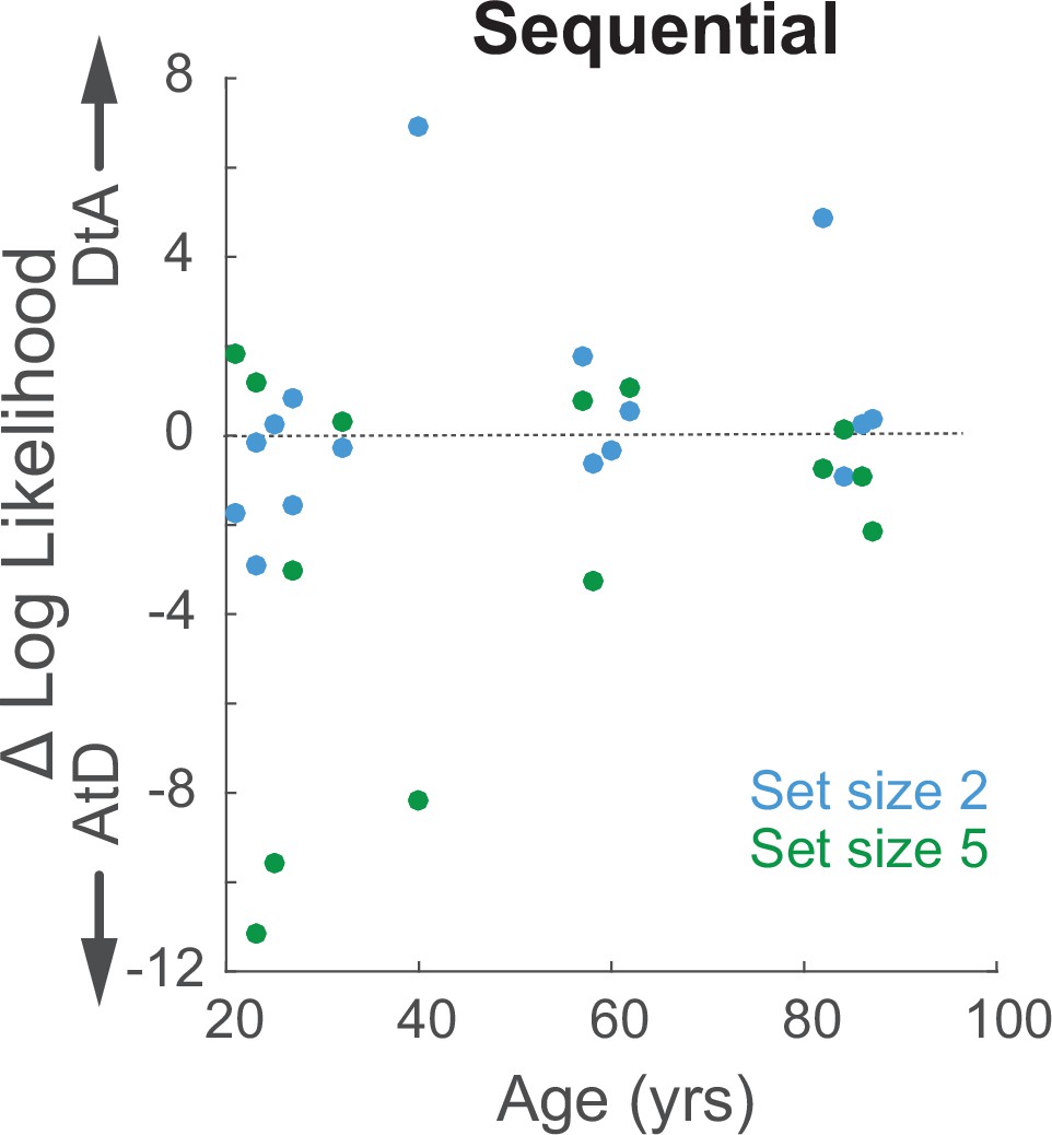
Relationship between log-likelihood difference for the two strategies and age for the Sequential condition.
Log-likelihood comparison for AtD and DtA (negative favors AtD) for set sizes 2 and 5 is not dependent upon age (correlation, ps>0.20 computed separately for each set size). AtD, Average-then-Diffuse; DtA, Diffuse-then-Average.
Author response image 1
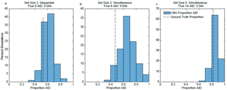
Results of VBA simulations compared to known ground truth.
a. For the set size 2, Sequential condition, VBA results tended to agree with the ground truth that neither strategy was more frequent (62% of simulations were within 10% of the ground truth). b. For the set size 2, Simultaneous condition, VBA results tended to disagree with the ground truth (only 23% of simulations were within 10% of the ground truth). c. For the set size 5, Simultaneous condition, VBA results tended to agree with the ground truth (90% of simulations were within 10% of the ground truth).
Tables
Table 1
Descriptions of all framework and model parameters.
Fit parameters are shown on the top. Derived parameters used in other analyses and descriptions are shown on the bottom. Variations used to model Sequential conditions are shown to the right.
| Fit model parameters(units) | Description | Variants for sequential conditions | Description | |
|---|---|---|---|---|
| η1 (deg2) | Static noise for a single item | |||
| ηN (deg2) | Static noise for N items | ηNE (deg2) | Static noise for Early items | |
| ηNL (deg2) | Static noise for Late items | |||
| ηMN (deg2) | Static noise for mean of N items | ηMN_seq (deg2) | Static noise for mean of N items in Sequential Conditions | |
| σ12 (deg2/s) | Diffusion constant tor single item | |||
| A (no units) | Diffusion cost of storing N items | |||
| Derived descriptive terms | ||||
| σN2 (deg2/s) | Diffusion constant for N items=σ12*NA | σNE2 (deg2/s) | Diffusion constant for Early items | |
| σNL2 (deg2/s) | Diffusion constant for Late items | |||
| σMN2 (deg2/s) | Diffusion constant for mean of N items | σMN_Seq2 (deg2/s) | Diffusion constant for mean of N items in Sequential Conditions | |
| AtD:=σ12 | DtA:= σ12*NA/N= σN2/N | |||
Table 2
Summary of model fits for the Simultaneous condition.
Parameters are: (1) η1, static noise for a single item; (2) ηN, static noise for N items; (3) ηMN, static noise for the mean of N items; (4) σ12, diffusion constant for a single item; and (5) A, diffusion cost for additional items. For each parameter, the maximum-likelihood estimates are given for the participants’ best fit by the indicated model (mean ± SEM across participants). * indicates t-test for H0: difference between the mean values of each parameter across models for a given set size=0, p<0.05.
| Set size (N) | Number best-fit participants | η1 | ηN | ηMN | σ12 | A | |
|---|---|---|---|---|---|---|---|
| AtD | 2 | 8 | 10.79±1.45 | 16.49±2.67 | 9.39±1.07 | 4.85±0.44 | 0.0892±0.24 |
| 5 | 14 | 9.80±1.18 | 36.88±5.33 | 14.79±1.50 | 4.34±0.47 | 0.0051±0.07* | |
| DtA | 2 | 9 | 8.22±1.35 | 14.16±3.13 | 10.45±2.09 | 3.67±0.58 | 0.61±0.22 |
| 5 | 3 | 7.63±0.30 | 45.49±17.03 | 21.10±7.59 | 5.14±0.28 | 0.49±0.14* |
Table 3
Summary of model fits for the Sequential condition.
Parameters are: (1) η1, non-time-dependent noise of a single value; (2) ηNE, non-time-dependent noise of the Early N–1 items; (3) ηNL, non-time-dependent noise of the Late Nth items; (4) ηMN-seq, non-time-dependent noise of the mean of N items; (5) σ12, diffusion constant of a single point; and (6) A, diffusion cost of additional items. For each parameter, the maximum likelihood estimates (mean over participants ± SEM) is given for the participants’ best fit with a particular model.
| Set size (N) | Number best-fit participants | η1 | ηNE | ηNL | ηMN-seq | σ12 | A | |
|---|---|---|---|---|---|---|---|---|
| AtD | 2 | 9 | 9.44 ± 1.47 | 20.32 ± 3.89 | 16.18 ± 3.16 | 14.02 ± 1.58 | 4.44 ± 0.73 | –0.34 ± 0.44 |
| 5 | 9 | 10.69 ± 1.21 | 37.06 ± 5.22 | 13.19 ± 2.06 | 15.94 ± 1.69 | 4.22 ± 0.73 | –0.09 ± 0.15 | |
| DtA | 2 | 8 | 10.25 ± 1.53 | 18.30 ± 3.31 | 17.43 ± 1.88 | 14.00 ± 3.11 | 4.58 ± 0.52 | –3.00 ± 2.58 |
| 5 | 8 | 9.11 ± 1.69 | 36.59 ± 5.54 | 22.27 ± 4.37 | 24.45 ± 4.60 | 4.43 ± 0.57 | –3.89 ± 2.90 |
Additional files
Download links
A two-part list of links to download the article, or parts of the article, in various formats.
Downloads (link to download the article as PDF)
Open citations (links to open the citations from this article in various online reference manager services)
Cite this article (links to download the citations from this article in formats compatible with various reference manager tools)
Strategy-dependent effects of working-memory limitations on human perceptual decision-making
eLife 11:e73610.
https://doi.org/10.7554/eLife.73610


