In vivo intraoral waterflow quantification reveals hidden mechanisms of suction feeding in fish
- Département Adaptations du Vivant, France
- Université de Paris, INSERM U1284, Center for Research and Interdisciplinarity (CRI), France
- Department of Biology, University of Antwerp, Universiteitsplein 1, Belgium
Figures
Figure 1
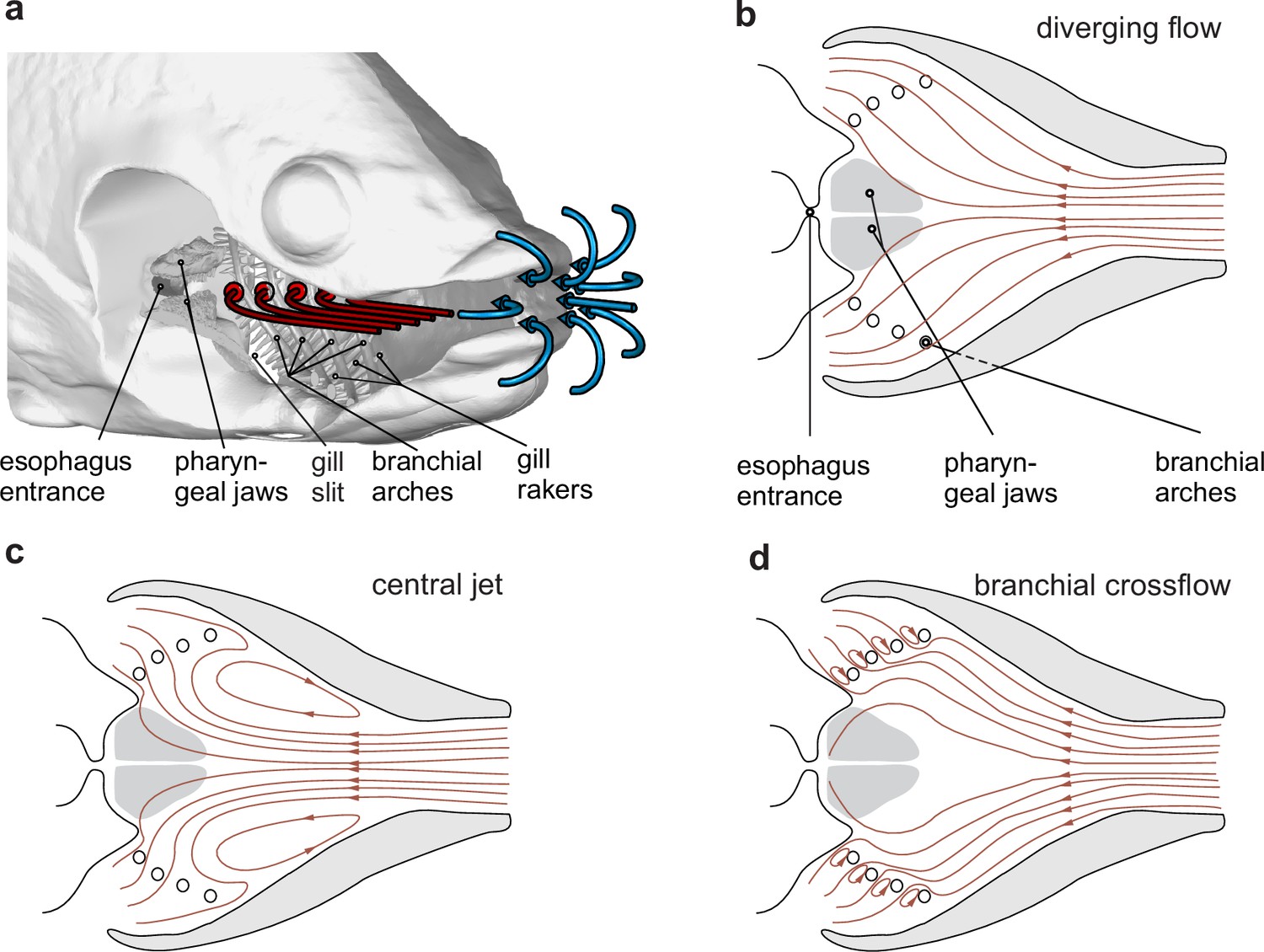
Hypothetical waterflow patterns during suction feeding in fish.
(a) Schematic illustration of extraoral flows (blue path line arrows) and hypothetical intraoral flows (red path line arrows) with important anatomical structures involved in food interception (the right-side buccopharyngeal walls and branchial basket are removed and only left-side path lines are shown) in a bony fish. (b–d) Three hypotheses for intraoral flow patterns, in a dorsoventral view. Note that from (b) to (d), the tendency to move food away from the desired food target, the esophagus, decreases.
Figure 2 with 3 supplements
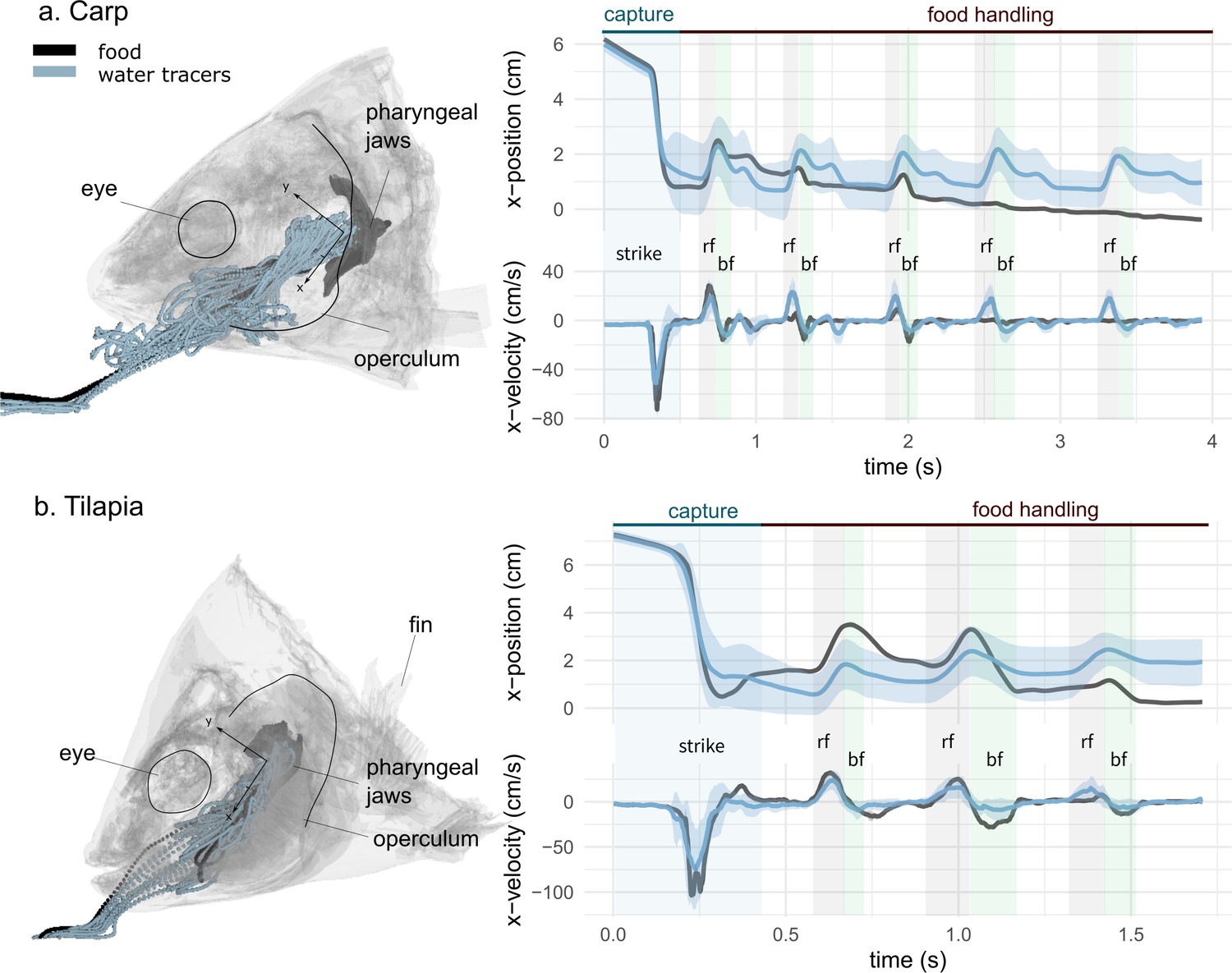
Representative sequences of suction feeding for carp (a) and tilapia (b).
Water and food tracer 3D trajectories outside and inside the buccal cavity are represented by a semi-transparent model of a carp (a, left) and a tilapia (b, left) head. The anteroposterior velocity of the water and food tracers of a carp (a, right) and a tilapia (b, right) over a representative suction-feeding sequence are shown, with the mean trajectory of the water tracers (blue line) surrounded by the standard deviation (lighter blue), as well as the trajectory of the food tracer (black). On the graphs, we show the division into two main phases: capture and intraoral food handling. During capture, the intake corresponds to a high negative magnitude for the anteroposterior velocity, followed by stasis, during which the anteroposterior velocity is close to zero. During intraoral food handling, we see an alternance of stasis consisting of a reverse flow (rf) with a positive anteroposterior velocity and of a backflow (bf) with a negative anteroposterior velocity of lower amplitudes compared to the first strike. (carp: two individuals, seven trials; tilapia: two individuals, six trials). The presented trials correspond to the X-ray videos (Figure 2—video 1, Figure 2—video 2).
-
Figure 2—source data 1
Normalized displacement components along the three cranium-bound orthogonal axes shown in Figure 2 (mean ± SD in %) for the food and water tracers in carp and tilapia.
- https://cdn.elifesciences.org/articles/73621/elife-73621-fig2-data1-v2.docx
-
Figure 2—source code 1
R code generating the graphs of Figure 2.
- https://cdn.elifesciences.org/articles/73621/elife-73621-fig2-code1-v2.zip
-
Figure 2—source code 2
R code identifying the phases during a suction-feeding sequence used in Figure 2.
- https://cdn.elifesciences.org/articles/73621/elife-73621-fig2-code2-v2.zip
Figure 2—figure supplement 1
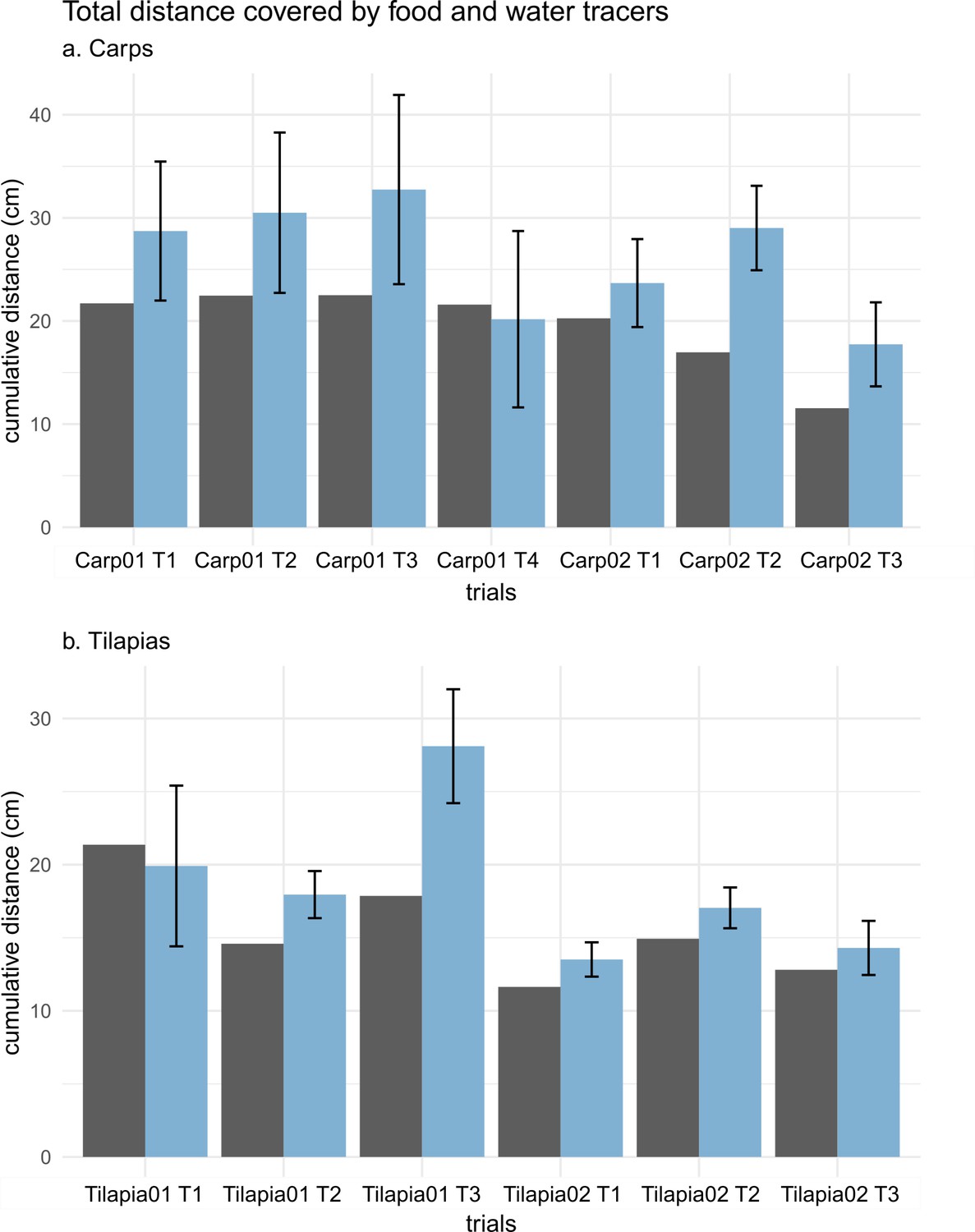
Histograms of the total distance covered by the food (in black) and the water tracers (in blue) during an entire sequence of suction feeding for each carp (a) and tilapia (b) trial.
-
Figure 2—figure supplement 1—source code 1
R code generating Figure 2—figure supplement 1.
- https://cdn.elifesciences.org/articles/73621/elife-73621-fig3-code3-v2.zip
Figure 2—video 1
Video of a suction-feeding sequence of a carp, showing the raw video, the water and food tracer trajectories, and the rigid-body reconstruction.
Figure 2—video 2
Video of a suction-feeding sequence of a tilapia, showing the raw video, the water and food tracer trajectories, and the rigid-body reconstruction.
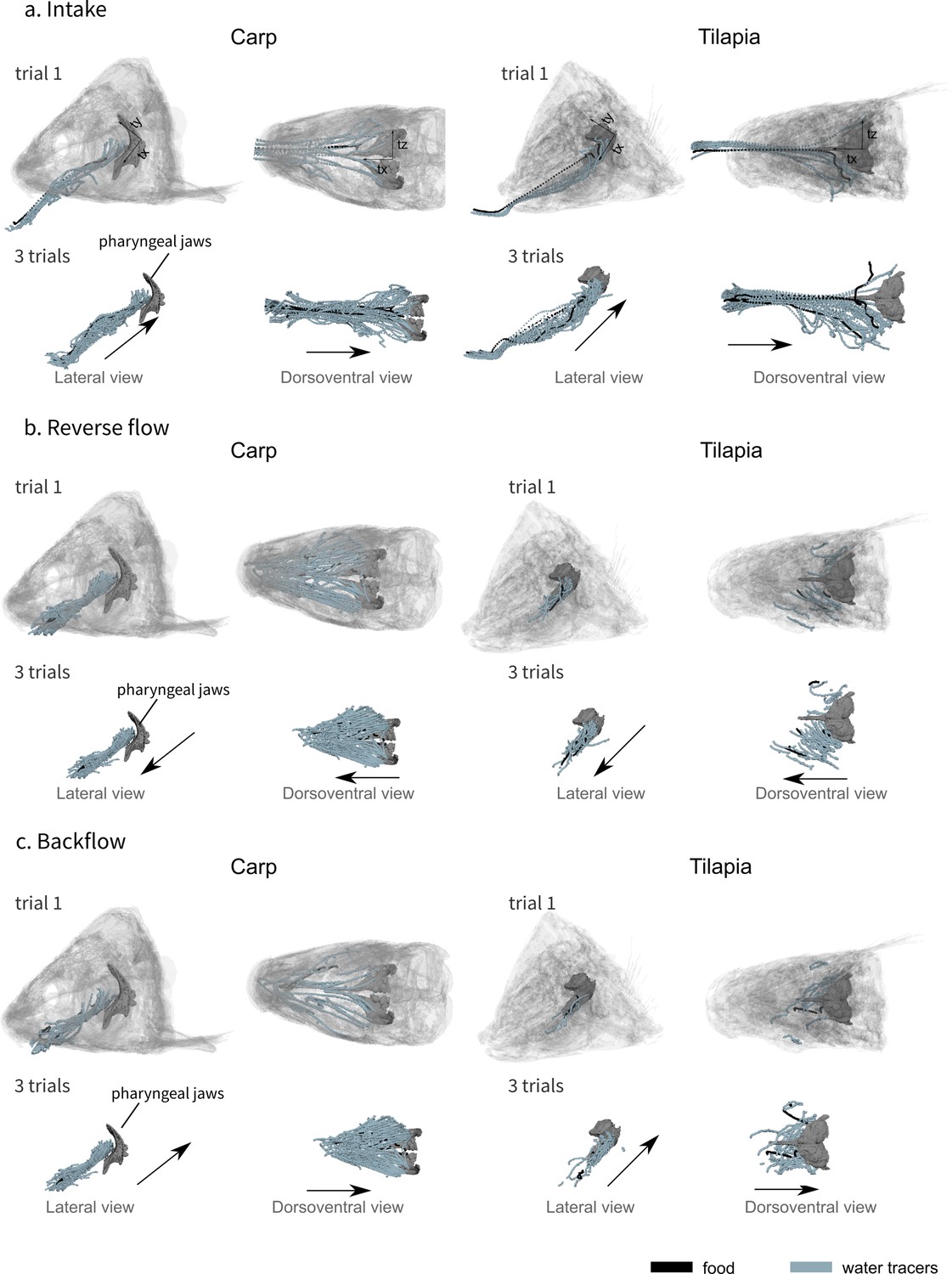
Figure 3 with 1 supplement
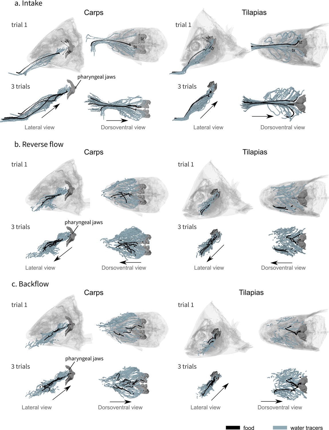
Visualization of the water tracer paths for both the lateral and dorsoventral views during the intake (a), the reverse flow (b), and the backflow (c).
A representative trial is presented on the first row of each phase and a combination of three trials for one individual of carp (carp 02) and three trials for one individual of tilapia (tilapia 01) on the second row of each phase, showing the consistency of the patterns. The axes are represented on the first row of schematics, the orientation remains the same for all the other schematics. The black arrows represent the global direction of tracer movement. The data for the other individuals of carp and tilapia is available in Figure 3—figure supplement 1.
Figure 3—figure supplement 1
Visualization of the water tracer paths for both the lateral and dorsoventral views during the intake (a), the reverse flow (b), and the backflow (c).
A representative trial is presented on the first row of each phase and a combination of three trials for one individual of carp (carp 01) and three trials for one individual of tilapia (tilapia 02) on the second row of each phase, showing the consistency of the patterns. The axes are represented on the first row of schematics, the orientation remains the same for all the other schematics. The black arrows represent the global direction of tracer movement.
Figure 4 with 2 supplements
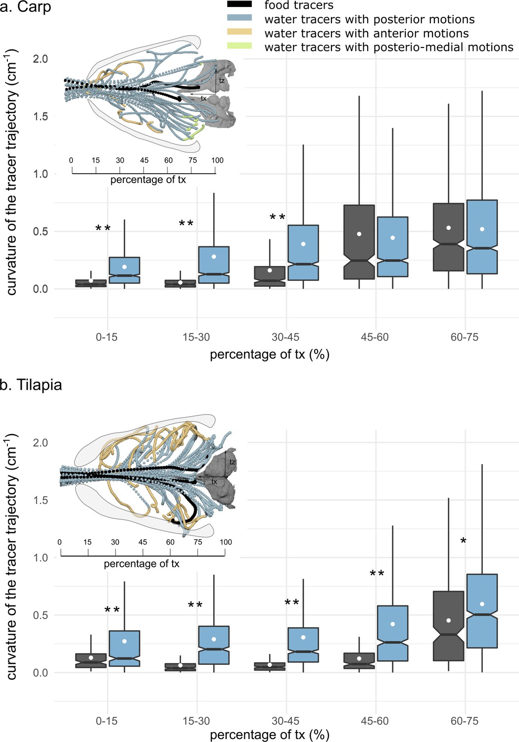
Boxplots of the mediolateral curvature calculated based on intervals of the anteroposterior trajectory during the intake in carp (a) and tilapia (b).
The lower and upper hinges correspond to the first and third quartiles (the 25th and 75th percentiles), and the white dot gives a 95% confidence interval for comparing medians. The asterisks represent the significance of the statistical tests comparing the water and food tracers’ curvatures (*p-value≤0.05, **p-value≤0.01) (carp: two individuals, seven trials; tilapia: two individuals, six trials). The schematics in the upper part of each subfigure correspond to a dorsoventral view of three trials of one individual of carp (a) and three trials of one individual of tilapia (b) showing the water (in blue, yellow, and green) and food tracer (in black) trajectories. The blue, yellow, and green trajectories highlight the posterior, anterior, and posteriomedial motions of the water tracers, respectively.
-
Figure 4—source code 1
R code generating the graphs of Figure 4.
- https://cdn.elifesciences.org/articles/73621/elife-73621-fig4-code1-v2.zip
Figure 4—figure supplement 1
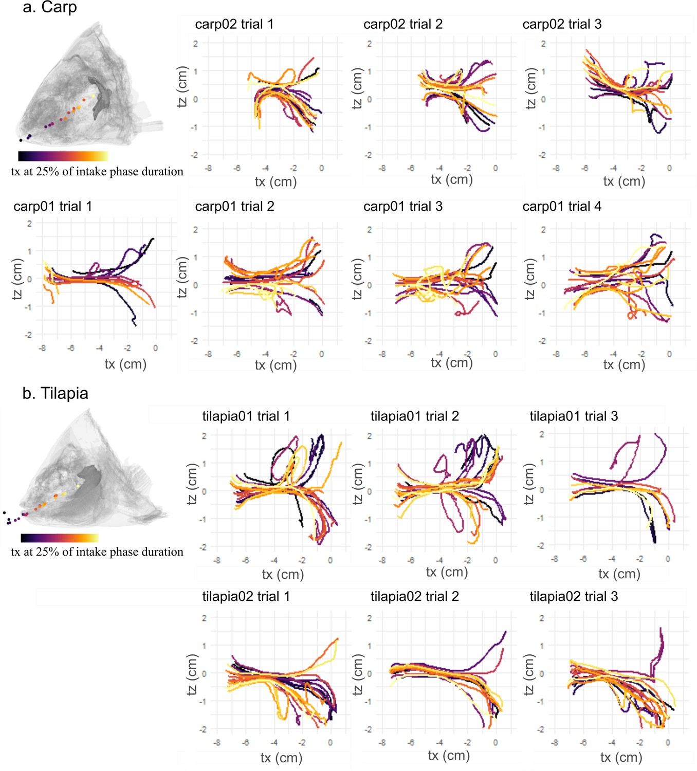
Visualization of the water tracer trajectories on a dorsoventral view (tx, tz) during the intake for the seven trials of carp 01 and carp 02 (a) and the six trials of tilapia 01 and tilapia 02 (b).
The diagrams represent a lateral view of carp 02 and tilapia 01 with the location of the water tracers at 25% of the intake phase duration with the matching color gradient, implying that tracers entering the buccal cavity at an early stage are displayed with light colors and those entering at a late stage in dark colors.
-
Figure 4—figure supplement 1—source code 1
R code generating the graphs of Figure 4—figure supplement 1.
- https://cdn.elifesciences.org/articles/73621/elife-73621-fig5-code5-v2.zip
Figure 4—figure supplement 2
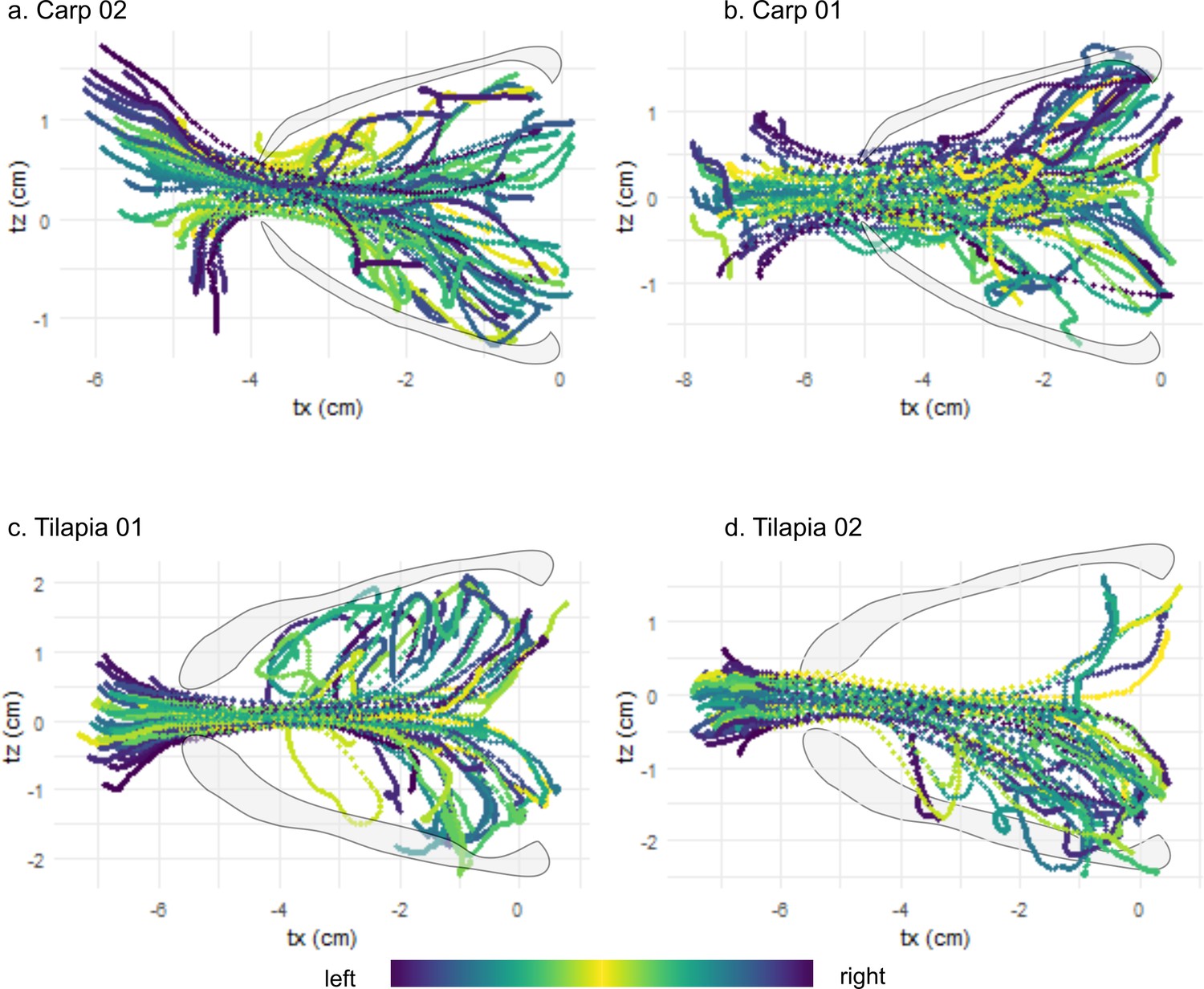
Visualization of the water tracer trajectories on a dorsoventral view (tx, tz) during the intake for the four trials of carp 01 (a), the three trials of carp 02 (b), the three trials of tilapia 01 (c), and the three trials of tilapia 02 (d).
The color gradient corresponds to the initial position of the tracer on the mediolateral axis (tz).
-
Figure 4—figure supplement 2—source code 1
R code generating the graphs of Figure 4—figure supplement 2.
- https://cdn.elifesciences.org/articles/73621/elife-73621-fig6-code6-v2.zip
Figure 5 with 1 supplement
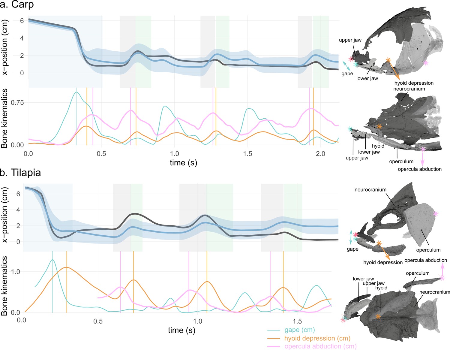
Water tracer anteroposterior trajectory, gape, hyoid depression, and opercula abduction during representative suction-feeding sequences in carp (a) and tilapia (b).
The shaded bars in the x-position graphs represent theintake (blue), reverse flow (rf, grey), and backflow (bf, green) phases. The vertical lines in the bone kinematic plots represent the time of the peak gape during the intake (in blue), peak hyoid depression (in orange), and peak opercula abduction (pink) during the rfs. The sketches on the right represent a lateral and ventral view of a carp (top) and a tilapia (bottom) with the location of the locators used to calculate the gape, hyoid depression, and opercula abduction. Note that the opercula were out of the field view at the beginning of the selected tilapia trial; therefore, the opercula abduction trace starts after the intake. See Figure 5—figure supplement 1 for the location of the implanted markers.
-
Figure 5—source code 1
R code generating the graphs of Figure 5.
- https://cdn.elifesciences.org/articles/73621/elife-73621-fig5-code1-v2.zip
Figure 5—figure supplement 1

Position of the implanted markers and the locators in the carp (a–d) and tilapia (e–h).
The lateral views (a, c, e, g), frontal views (b, f), and dorsal views (d, h). The pharyngeal jaws are transparent, the implanted markers are in black, and the locators added to the rigid bodies are in color.
Figure 6 with 1 supplement
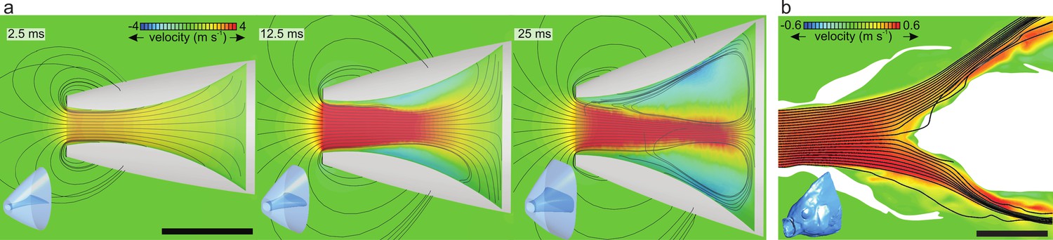
Results from previous computational fluid dynamics (CFD) studies of suction feeding in fish showing intraoral flow patterns.
Anterior-to-posterior velocities (color scale) and streamlines at the mid-frontal section planes are given, with the respective 3D models of the head in the bottom-left corners. (a) Central jet development in a CFD model of suction feeding in shiner perch (Cymatogaster aggregata) from Thompson et al., 2018 showing flow patterns at three consecutive instants during suction-feeding event (see Figure 6—video 1). (b) Model of steady flow into the mouth of a scan-based reconstruction of the head of a sunfish (Lepomis gibbosus) indicating approximately stagnant water (in green) close to the opercula and a jet shearing the posterior pharynx before exiting the cavity (after Provini and Van Wassenbergh, 2018). Scale bar, 10 mm.
Figure 6—video 1
Video showing the central jet development in a computational fluid dynamics (CFD) model of suction feeding in shiner perch (Cymatogaster aggregata) from Thompson et al., 2018 showing flow patterns at three consecutive instants during suction-feeding event.
Figure 7
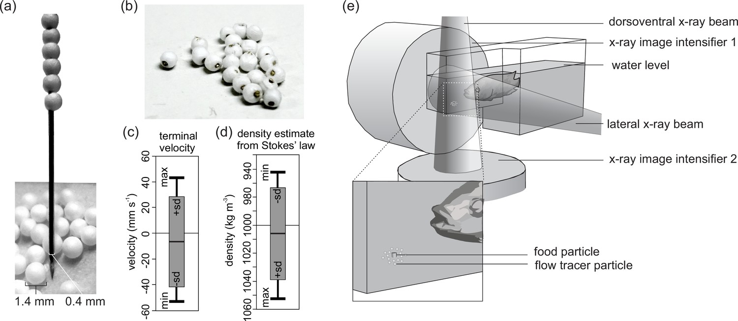
Tracer fabrication for X-ray particle tracking and the experimental design.
(a) Construction of the flow tracer particles by piercing 1.4-mm-diameter expanded polystyrene (EPS) spheres on a 0.4-mm-diameter, Vaseline-coated brass rod with a sharpened tip. (b) Flow tracers after cutting the rod. (c) Terminal velocity test results of the EPS brass flow tracers released in water (positive velocities: rising; negative velocities: sinking), and (d) the corresponding estimates of density based on Stokes’ law (see Materials and methods for details) (N = 19). (e) Experimental design indicating X-ray beam, image intensifier orientation, and placement of the food surrounded by flow tracer particles at the bottom of the narrow extrusion of the aquarium.
-
Figure 7—source code 1
R code generating the graphs of Figure 7.
- https://cdn.elifesciences.org/articles/73621/elife-73621-fig7-code1-v2.zip
Figure 8 with 1 supplement
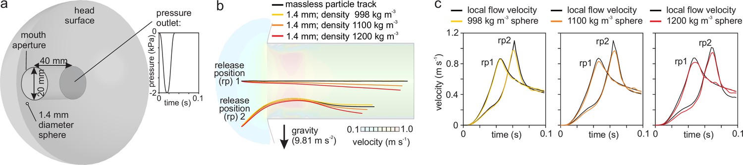
Numerical modeling assessment of tracking performance of suction-feeding waterflows.
(a) Cylindrical mouth cavity inside a hemispherical head generating suction trough a transient pressure-outlet-type boundary condition assigned to the back of the cylinder. (b) Path lines of the water (black lines) released from two points in front of the mouth aperture (rp 1 and 2) in comparison with trajectories from 1.4-mm-diameter spheres with density equal to the water (998 kg/m3; yellow) and two cases with negative buoyancy (1100 kg/m3, orange; 1200 kg/m3, red). Note that the direction of gravity is downward. Flow velocity color maps are shown for the simulation time of 0.06 s (see Figure 8—video 1). (c) Comparison of the velocity between the particles (colored lines) and waterflow at the current position of the particles in a flow simulation in the absence of the particle (black lines).
Figure 8—video 1
Video of the computational fluid dynamics (CFD) simulation testing the influence of the tracer density on their trajectory during the intake.
Additional files
Download links
A two-part list of links to download the article, or parts of the article, in various formats.
Downloads (link to download the article as PDF)
Open citations (links to open the citations from this article in various online reference manager services)
Cite this article (links to download the citations from this article in formats compatible with various reference manager tools)
In vivo intraoral waterflow quantification reveals hidden mechanisms of suction feeding in fish
eLife 11:e73621.
https://doi.org/10.7554/eLife.73621


