Bayesian machine learning analysis of single-molecule fluorescence colocalization images
- Department of Biochemistry, Brandeis University, United States
Figures
Figure 1
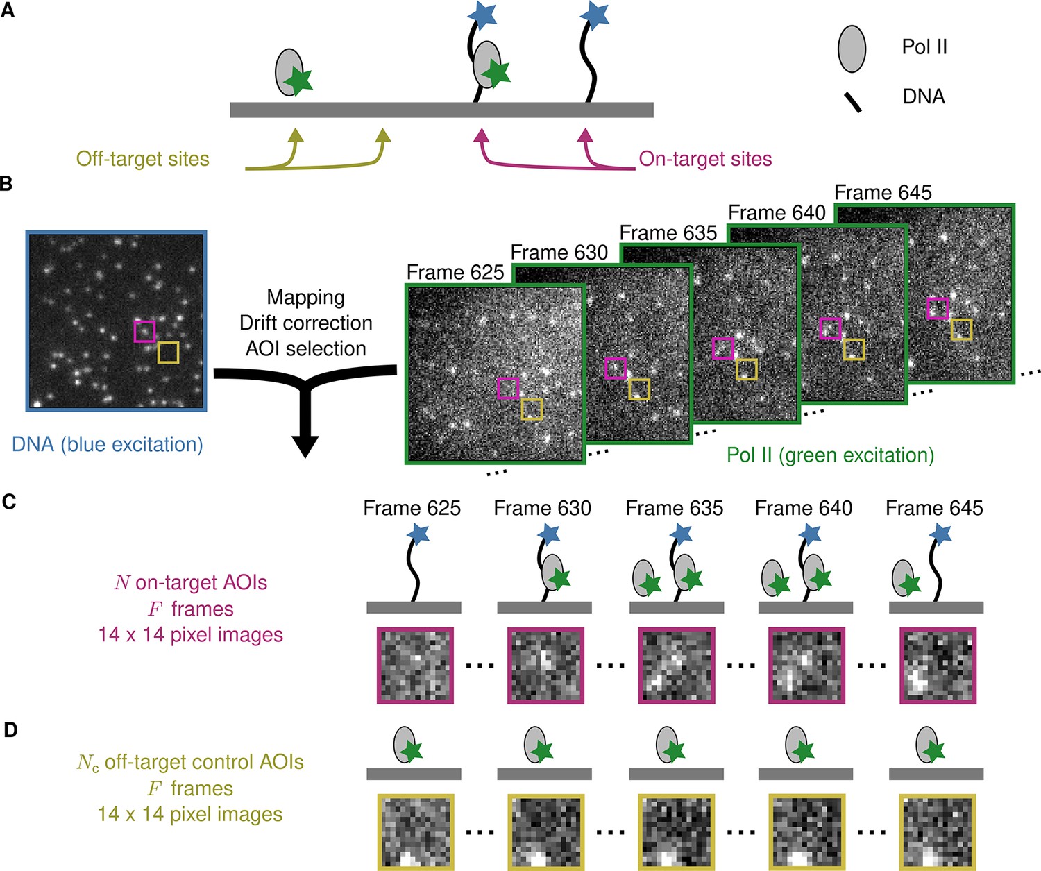
Example CoSMoS experiment.
(A) Experiment schematic. DNA target molecules labeled with a blue-excited fluorescent dye (blue star) are tethered to the microscope slide surface. RNA polymerase II (Pol II) binder molecules labeled with a green-excited dye (green star) are present in solution. (B) Data collection and preprocessing. After collecting a single image with blue excitation to identify the locations of the DNA molecules, a time sequence of Pol II images was collected with green excitation. Preprocessing of the images includes mapping of the corresponding points in target and binder channels, drift correction, and identification of two sets of areas of interest (AOIs). One set corresponds to locations of target molecules (e.g., purple square); the other corresponds to locations where no target is present (e.g., yellow square). (C) On-target data. Data are time sequences of 14 × 14 pixel AOI images centered at each target molecule. Frames show presence of on-target (e.g., frame 630) and off-target (e.g., frame 645) Pol II molecules. (D) Off-target control data. Control data consists of images collected from randomly selected sites at which no target molecule is present. Such sites can be AOIs in which no fluorescent target molecule is visible (e.g., the yellow square in the DNA channel shown in B). Alternatively, control data can be taken from a recording of a separate control sample to which no target molecules were added. Image data in B, C, and D is from Data set A in Table 1.
Figure 2 with 2 supplements
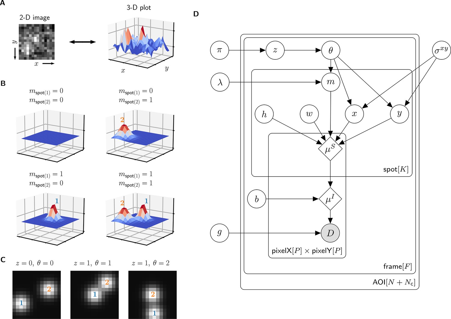
Depiction of the cosmos probabilistic image model and model parameters.
(A) Example AOI image (from Data set A in Table 1). The AOI image is a matrix of 14 × 14 pixel intensities which is shown here as both a 2-D grayscale image and as a 3-D intensity plot. The image contains two spots; one is centered at target location (image center) and the other is located off-target. (B) Examples of four idealized noise-free image representations (). Image representations consist of zero, one, or two idealized spots () superimposed on a constant background (). Each fluorescent spot is represented as a 2-D Gaussian parameterized by integrated intensity (), width (), and position (, ). The presence of spots is encoded in the binary spot existence indicator . (C) Simulated idealized images illustrating different values of the target-specific spot state parameter and index parameter . = 0 corresponds to a case when no specifically bound molecule is present ( = 0); = 1 or 2 corresponds to the cases in which specifically bound molecule is present ( = 1) and corresponds to spot 1 or 2, respectively. (D) Condensed graphical representation of the cosmos probabilistic model. Model parameters are depicted as circles and deterministic functions as diamonds. Observed image () is represented by a shaded circle. Related nodes are connected by edges, with an arrow pointing towards the dependent node (e.g., the shape of each 2-D Gaussian spot depends on spot parameters , , , , and ). Plates (rounded rectangles) contain entities that are repeated for the number of instances displayed at the bottom-right corner: number of total AOIs (), frame count (), and maximum number of spots in a single image ( = 2). Parameters outside of the plates are global quantities that apply to all frames of all AOIs. A more complete version of the graphical model specifying the relevant probability distributions is given in Figure 2—figure supplement 1.
Figure 2—figure supplement 1
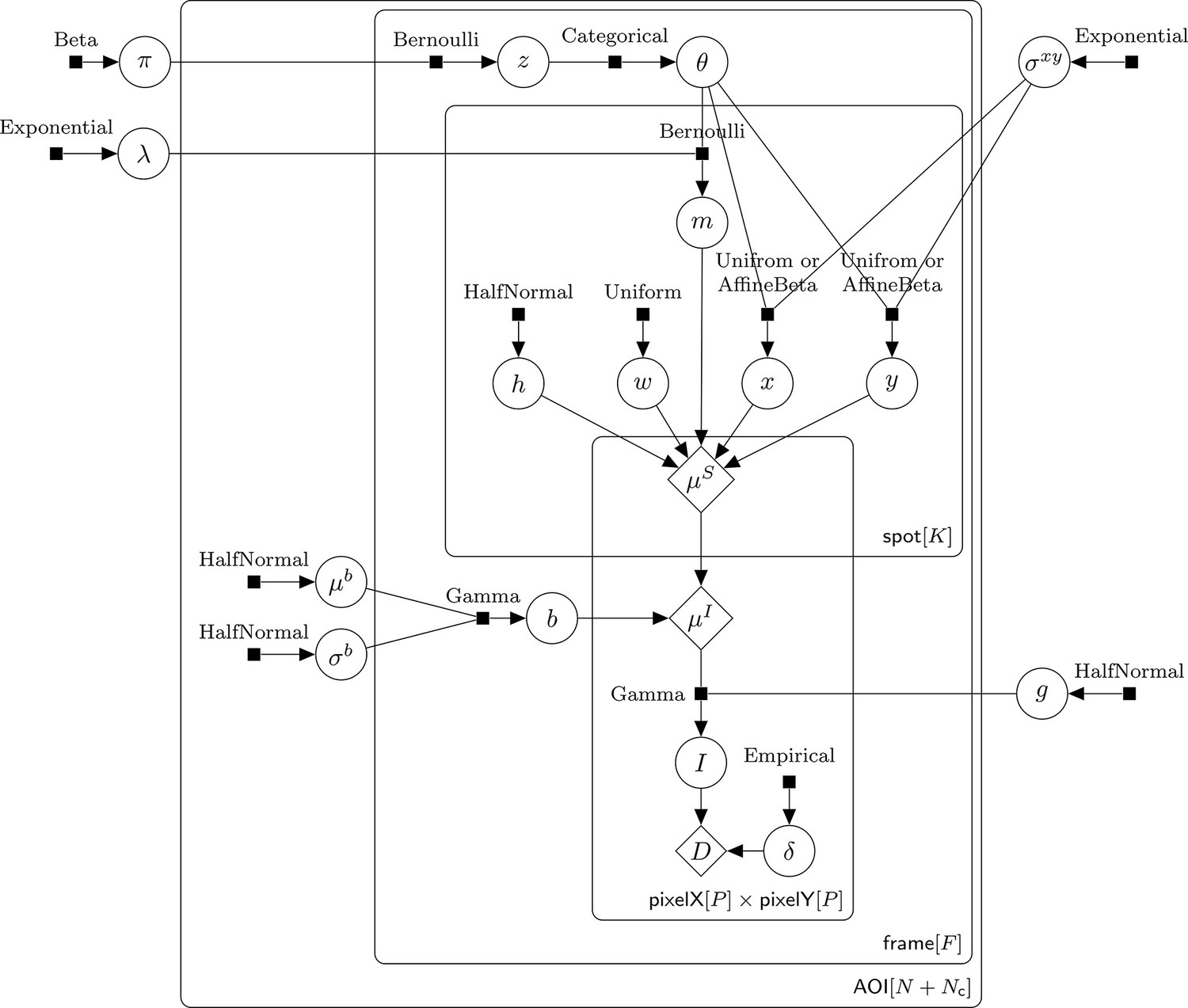
Extended graphical representation of the generative probabilistic model.
Directed factor graph representation (Bishop, 2006) of model parameters and parameter distributions. This diagram is a more complete version of the graphical model shown in Figure 2D; it includes additional parameters (, ) and explicitly specifies the relevant probability distributions. Model parameters are depicted as circles, parameter distributions as small filled squares, and deterministic functions as diamonds. Names of the probability distributions are written next to the squares. Input parameters and output parameters are connected by lines, with an arrow pointing towards the dependent parameter. Observed AOI image () is the sum of the noisy photon-dependent image () and the photon-independent camera offset (). Plates (rounded rectangles) contain nodes that are repeated for the number of instances displayed at the bottom-right corner: number of AOIs (), frame count (), maximum number of spots in a single image (), and number of image pixels (). The prior for and is Uniform for target-nonspecific spots and AffineBeta for target-specific spots (see Figure 2—figure supplement 2).
Figure 2—figure supplement 2
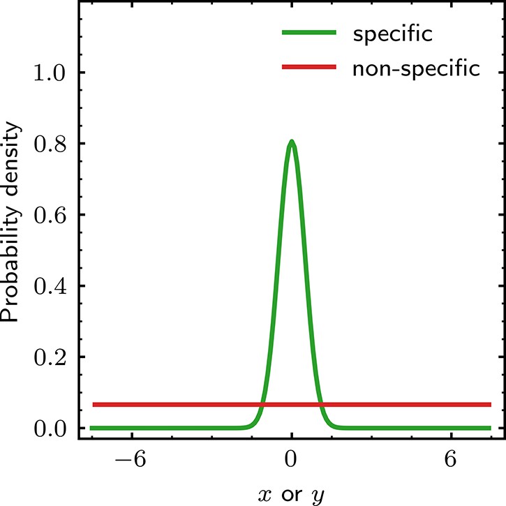
Prior distributions for the and spot position parameters.
Prior distributions of and for specific and non-specific binding. Probability densities for and are defined in the range relative to the target molecule and are conditional on the identity of the spot (specific or non-specific). The width of the peak in the specific distribution is given by , the value of which is learned from the data. Probability densities for and are identical.
Figure 3 with 4 supplements

Tapqir analysis and inferred model parameters.
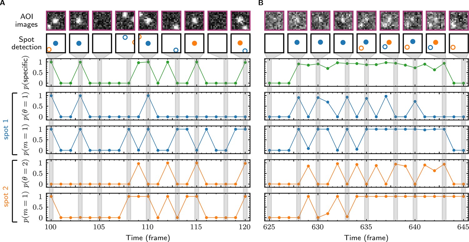
(A,B) Tapqir was applied to simulated data (lamda0.5 parameter set in Supplementary file 1) (A) and to experimental data (Data set A in Table 1) (B). (A) and (B) each show a short extract from a single target location in the data set. The first row shows AOI images for the subset of frames indicated by gray shaded stripes in the plots; image contrast and offset settings are consistent within each panel. The second row shows the locations of spots determined by Tapqir. Spot numbers 1 (blue) and 2 (orange) are assigned arbitrarily and may change from fame to frame. For clarity, only data for spots with a spot probability > 0.5 are shown. Spots predicted to be target-specific ( > 0.5 for spot ) are shown as filled circles. The topmost graphs (green) show the calculated probability that a target-specific spot is present () in each frame. Below are the calculated spot intensities (), spot widths (), and locations (, ) for spot 1 (blue) and spot 2 (orange), and the AOI background intensities (). Again, for clarity data are only shown for likely spots ( > 0.5). Error bars: 95% CI (credible interval) estimated from a sample size of 500. Some error bars are smaller than the points and thus not visible.
Figure 3—figure supplement 1
Calculated spot probabilities.
The data sets used for panels A and B are identical to those in Figure 3A and B; the first two rows and the (green) graph are reproduced from that figure. Blue graphs show the probability of being present () and of being target-specific () for the arbitrarily designated spot 1 in each frame. Orange graphs show the analogous quantities and for spot 2. For a given image, the probability that any target-specific spot is present is equal to .
Figure 3—figure supplement 2
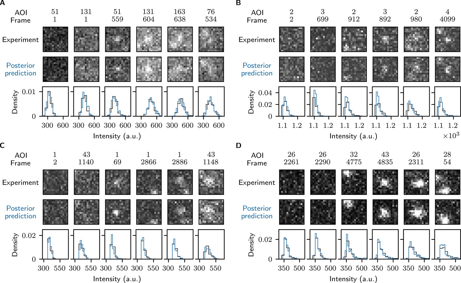
Reproduction of experimental data by posterior predictive sampling.
Example frames are shown from Data set A (A: SNR = 1.61), Data set B (B: SNR = 3.77), Data set C (C: SNR = 4.23), and Data set D (D: SNR = 3.06) in Table 1. In each panel the top row shows AOI images selected from the experimental data and middle row shows corresponding images obtained by sampling from the posterior distributions. Image contrast and offset are consistent within each panel. The bottom row shows pixel intensity distributions from the experimental and posterior prediction images.
Figure 3—figure supplement 3
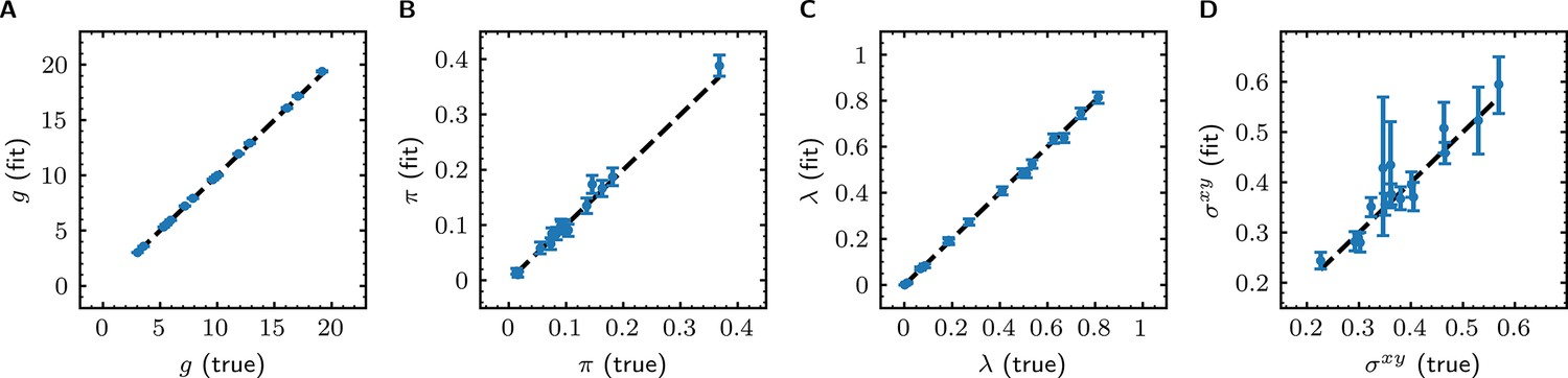
Tapqir analysis of image data simulated using a broad range of global parameters.
Simulations (see Materials and methods) consist of 16 data sets where values of global parameters (, , and ) were randomly generated for each data set (Supplementary file 2). Simulated data were fit with Tapqir, and parameter values from the fit (with 95% credible interval estimated from a sample size of 10,000) are plotted against the true parameter values. To guide the eye, dashed lines indicate identical true and fit values. (A) Gain of the camera . (B) Average target-specific binding probability . (C) Target non-specific binding density . (D) Proximity parameter .
Figure 3—figure supplement 4
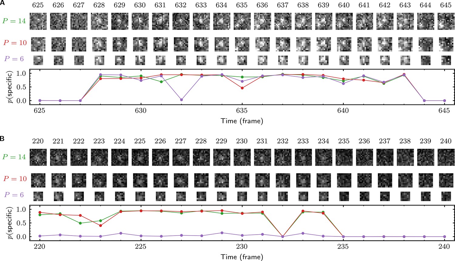
Effect of AOI size on analysis of experimental data.
(A) and (B) each show a short extract from a single target location (AOI 163 in (A) and AOI 0 in (B)) from Data set A (Table 1; SNR = 1.61). Tapqir was applied to the data set using AOI image sizes of 14 × 14 (first row), 10 × 10 (second row), and 6 × 6 (third row) pixels. Corresponding output probabilities are plotted in the graph. Image contrasts in (A) and (B) are different. Unattended calculation time on an AMD Ryzen Threadripper 2990 WX with an Nvidia GeForce RTX 2080Ti GPU using CUDA version 11.5 for the different AOI sizes were: 7 h 40 min ( = 14), 3 h 5 min ( = 10), and 2 h 40 min ( = 6).
Figure 4 with 1 supplement
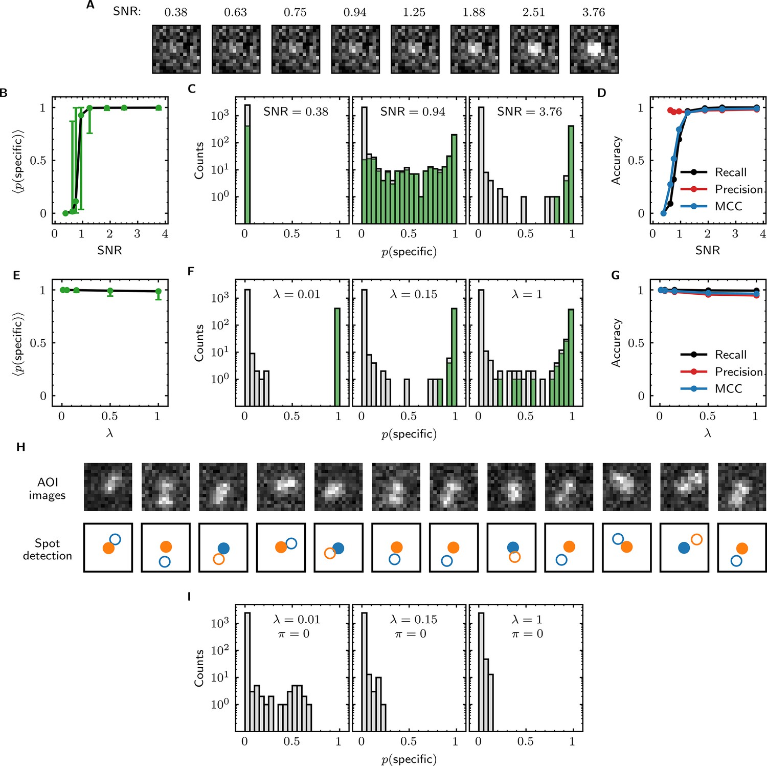
Tapqir performance on simulated data with different SNRs or different non-specific binding densities.
(A–D) Analysis of simulated data over a range of SNR. SNR was varied in the simulations by changing spot intensity while keeping other parameters constant (Supplementary file 3). (A) Example images showing the appearance of the same target-specific spot simulated with increasing SNR. (B) Mean of Tapqir-calculated target-specific spot probability (with 95% CI; see Materials and methods) for the subset of images where target-specific spots are known to be present. (C) Histograms of for selected simulations with SNR indicated. Data are shown as stacked bars for images known to have (green, 15%) or not have (gray, 85%) target-specific spots. Count is zero for bins where bars are not shown. (D) Accuracy of Tapqir image classification with respect to presence/absence of a target-specific spot. Accuracy was assessed by MCC, recall, and precision (see Results and Materials and methods sections). (E–G) Same as in (B–D) but for the data simulated over a range of non-specific binding densities at fixed SNR = 3.76 (Supplementary file 1). (H) Spot recognition in AOI images containing closely spaced target-specific and non-specific spots. Images were selected from the = 1 data set in (E–G). AOI images and spot detection are plotted as in Figure 3, with spot numbers 1 (blue) and 2 (orange) assigned arbitrarily and spots predicted to be target-specific shown as filled circles. (I) Same as in (C) but for the data simulated over a range of non-specific binding densities with no target-specific binding ( = 0) (Supplementary file 4).
Figure 4—figure supplement 1
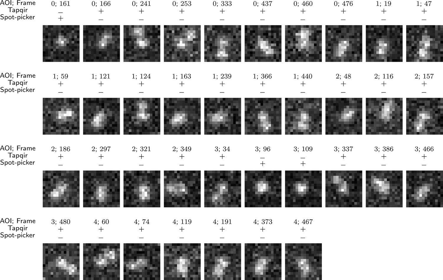
False negative spot misidentifications by Tapqir and spot-picker method.
The same = 1 simulated data set used in Figure 4E–H (lamda1 in Supplementary file 1) was analyzed by Tapqir and spot-picker. The data set contained 418 AOI images containing target-specific spots, of which the 37 shown here were falsely predicted to contain no target-specific spot (3 by Tapqir and 34 by spot-picker). Correct (+) and incorrect (−) predictions by each program are indicated. In all AOI images except AOI 3 frame 109, there is a nearby target non-specific spot in addition to the target-specific one. False negative classifications by spot-picker method are presumably due to the presence of a closely located target non-specific spot that distorts the shape of a target-specific spot. Tapqir, on the other hand, is able to correctly infer the presence of two closely located spots even when they are not completely resolved (Figure 4H). The rare (3 out of 418) false negative classifications by Tapqir likely arise from target-specific spots with centers that deviate from the target location by much more (∼ 0.7 pixels) than the inferred proximity parameter ( = 0.2 pixels).
Figure 5

Tapqir analysis of association/dissociation kinetics and thermodynamics.
(A) Chemical scheme for a one-step association/dissociation reaction at equilibrium with pseudo-first-order binding and dissociation rate constants and , respectively. (B) A simulation of the reaction in (A) and scheme for kinetic analysis of the simulated data with Tapqir. The simulation used SNR = 3.76, = 0.02 s−1, = 0.2 s−1, and a high target-nonspecific binding frequency = 1 (Supplementary file 5, data set kon0.02lamda1). Full dataset consists of 100 AOI locations and 1,000 frames each for on-target data and off-target control data. Shown is a short extract of on-target data from a single AOI location in the simulation. Plots show simulated presence/absence of the target-specific spot (blue) and Tapqir-calculated estimate of corresponding target-specific spot probability (green). Two thousand binary traces (e.g., black records) were sampled from the posterior distribution and used to infer and using a two-state hidden Markov model (HMM) (see Materials and methods). Each sample trace contains well-defined time intervals corresponding to target-specific spot presence and absence (e.g., and ). (C,D,E) Kinetic and equilibrium constants from simulations (Supplementary file 5) using a range of values and target-nonspecific spot frequencies , with constant = 0.2 s−1. (C) Values of used in simulations (blue) and mean values (and 95% CIs, black) inferred by HMM analysis from the 2000 posterior samples. Some error bars are smaller than the points and thus not visible. (D) Same as (C) but for . (E) Binding equilibrium constants used in simulation (blue) and inferred from Tapqir-calculated π as (black).
Figure 6 with 3 supplements
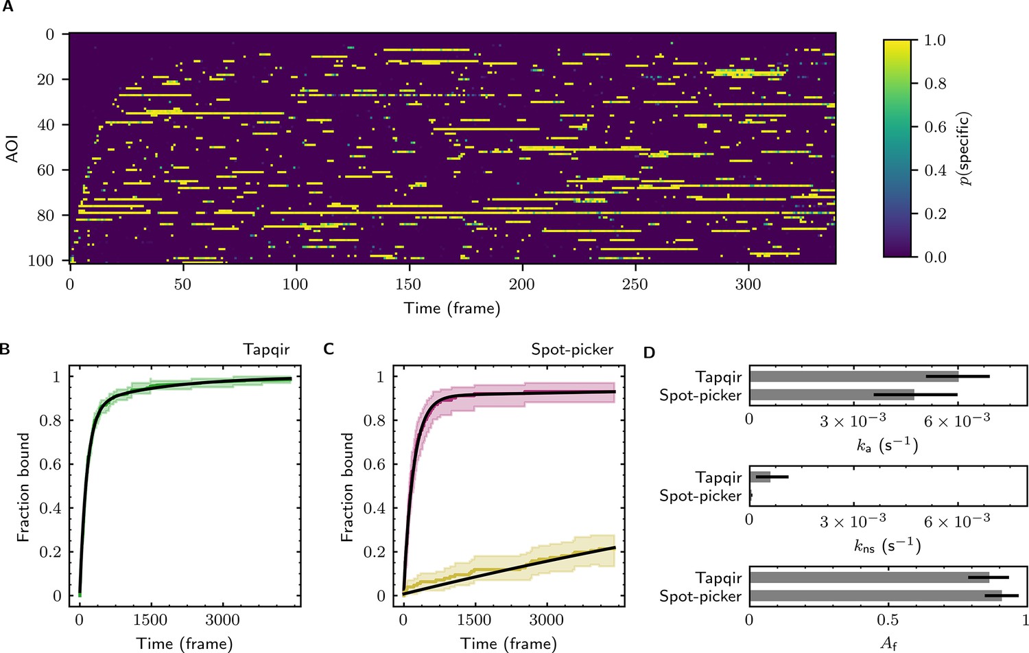
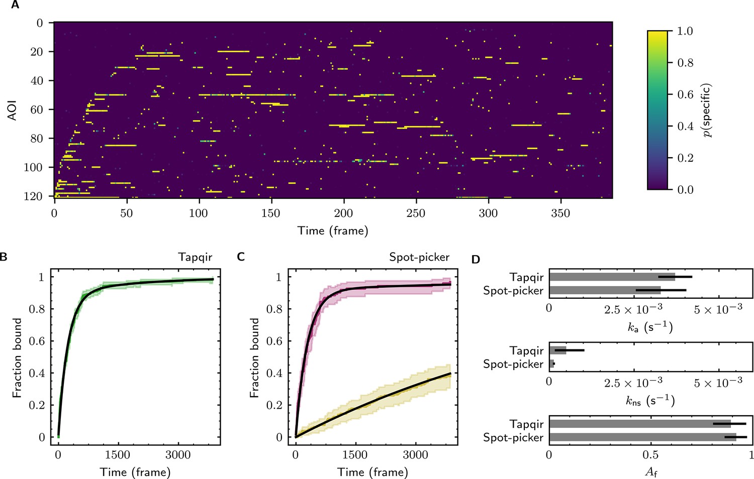
Extraction of target-binder association kinetics from example experimental data.
Data are from Data set B (SNR = 3.77, = 0.1575; see Table 1). (A) Probabilistic rastergram representation of Tapqir-calculated target-specific spot probabilities (color scale). AOIs were ordered by decreasing times-to-first-binding. For clarity, only every thirteenth frame is plotted. (B) Time-to-first-binding distribution using Tapqir. Plot shows the cumulative fraction of AOIs that exhibited one or more target-specific binding events by the indicated frame number (green) and fit curve (black). Shading indicates uncertainty. (C) Time-to-first-binding distribution using an empirical spot-picker method Friedman et al., 2013. The spot-picker method jointly fits first spots observed in off-target control AOIs (yellow) and in on-target AOIs (purple) yielding fit curves (black). (D) Values of kinetic parameters , , and (see text) derived from fits in (B) and (C). Uncertainties reported in (B, C, D) represent 95% credible intervals for Tapqir and 95% confidence intervals for spot-picker (see Materials and methods).
Figure 6—figure supplement 1
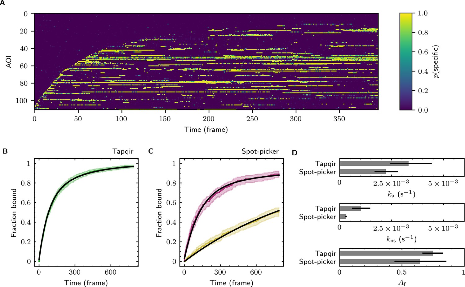
Additional example showing extraction of target-binder association kinetics from experimental data.
Figure 6—figure supplement 2
Additional example showing extraction of target-binder association kinetics from experimental data.
Figure 6—figure supplement 3

Additional example showing extraction of target-binder association kinetics from experimental data.
Figure 7
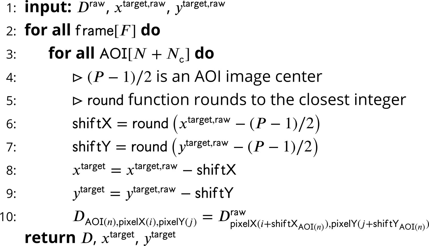
Extraction of AOI images from raw images.
-
Figure 7—source data 1
Original text for Figure 7.
- https://cdn.elifesciences.org/articles/73860/elife-73860-fig7-data1-v2.pdf
Figure 8
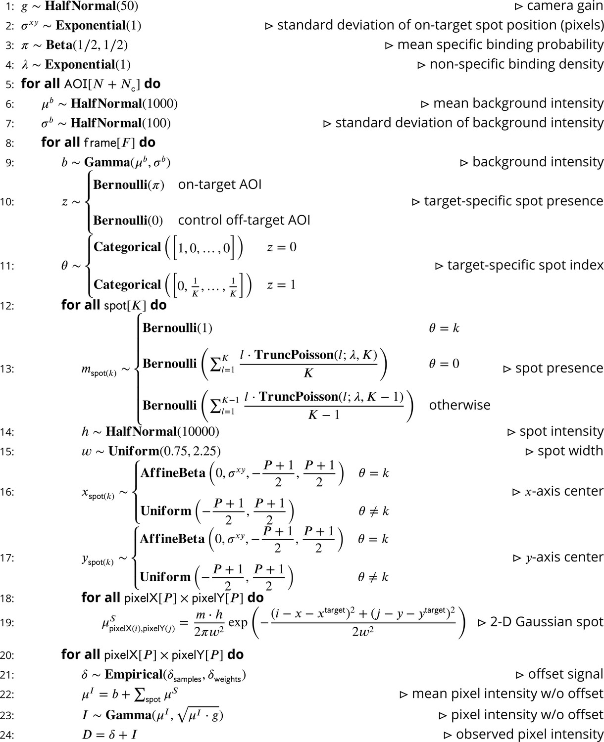
Pseudocode representation of cosmos model.
-
Figure 8—source data 1
Original text for Figure 8.
- https://cdn.elifesciences.org/articles/73860/elife-73860-fig8-data1-v2.pdf
Figure 9

Pseudocode representation of cosmos guide.
-
Figure 9—source data 1
Original text for Figure 9.
- https://cdn.elifesciences.org/articles/73860/elife-73860-fig9-data1-v2.pdf
Tables
Table 1
Experimental data sets.
| Data set sizea | SNR | π [95% CI] | λ [95% CI] | g [95% CI] | σxy [95% CI] | Compute time |
|---|---|---|---|---|---|---|
| Data set A: Binder, SNAPf-tagged S. cerevisiae RNA polymerase II labeled with DY549; Target, transcription template DNA containing 5× Gal4 upstream activating sequences and CYC1 core promoter; Conditions, yeast nuclear extract supplemented with Gal4-VP16 activator and NTPs. From Rosen et al., 2020. | ||||||
| = 331, = 526, = 790 | 1.61 | 0.0951 [0.0936, 0.0966] | 0.2943 [0.2924, 0.2963] | 6.645 [6.643, 6.647] | 0.577 [0.573, 0.580] | 7 h 40 mb 3 h 50 mc |
| Data set B: Binder, 0.1 nM E. coli σ54 RNA polymerase labeled with Cy3; Target, 852 bp DNA containing the glnALG promoter; Conditions, physiological buffer, no NTPs. From (Fig. 1E) of Friedman et al., 2013. | ||||||
| = 102, = 127, = 4407 | 3.77 | 0.0846 [0.0835, 0.0857] | 0.1575 [0.1569, 0.1583] | 11.861 [11.856, 11.865] | 0.476 [0.474, 0.479] | 7 h 40 mb |
| Data set C: Binder, 0.4 nM E. coli σ54 RNA polymerase labeled with Cy3; Target, 3,591 bp DNA containing the glnALG promoter; Conditions, physiological buffer, no NTPs. From (Fig. 3D) of Friedman et al., 2013. | ||||||
| = 122, = 157, = 3855 | 4.23 | 0.0267 [0.0262, 0.0273] | 0.0876 [0.0869, 0.0883] | 16.777 [16.773, 16.782] | 0.404 [0.399, 0.408] | 9 h 15 mb |
| Data set D: Binder, 0.15 nM E. coli Cy3-GreB; Target, reconstituted backtracked EC-6 E. coli transcription elongation complex; Conditions, physiological buffer, no NTPs. Randomly selected subset of data set from Tetone et al., 2017. | ||||||
| = 200, = 200, = 5622 | 3.06 | 0.0038 [0.0036, 0.0039] | 0.0437 [0.0434, 0.0440] | 18.727 [18.724, 18.731] | 0.451 [0.438, 0.463] | 11 hb |
-
*N - number of on-target AOIs, Nc - number of control off-target AOIs, F - number of frames.
-
bUnattended calculation time on an AMD Ryzen Threadripper 2990WX with an Nvidia GeForce RTX 2080Ti GPU using CUDA version 11.5.
-
cUnattended calculation time on an Intel Xeon CPU with an Nvidia Tesla V100-SXM2-16GB GPU using CUDA version 11.2 in a Google Colab Pro account.
Table 2
The effect of AOI size on classification accuracy*.
-
*
Tapqir was applied to the same simulated data set (height1000 parameter set in Supplementary file 3; SNR = 1.25) using different AOI sizes.
-
†
The width () of the simulated spots (one standard deviation of the 2-D Gaussian) is equal to 1.4 pixels.
-
‡
Unattended calculation time on an AMD Ryzen Threadripper 2990WX with an Nvidia GeForce RTX 2080Ti GPU using CUDA version 11.5.
Table 3
Variables used in the Tapqir model.
| Symbol | Meaning | Domain |
|---|---|---|
| Maximum number of spots per image | ||
| Number of on-target AOIs | ||
| Number of off-target control AOIs | ||
| Number of frames | ||
| Size of the AOI image in pixels | ||
| Camera gain | ||
| Proximity | ||
| Average target-specific binding probability | ||
| Target-nonspecific binding density | ||
| Mean background intensity across AOI | ||
| Standard deviation of background intensity across AOI | ||
| Background intensity | ||
| Target-specific spot presence | ||
| Target-specific spot index | ||
| Spot presence indicator | ||
| Integrated spot intensity | ||
| Spot width | ||
| Center of the spot on the -axis | ||
| Center of the spot on the -axis | ||
| 2-D Gaussian spot | ||
| Ideal image w/o offset | ||
| Offset signal | ||
| Observed image w/o offset signal | ||
| Observed image () | ||
| Target molecule position on the -axis | ||
| Target molecule position on the -axis | ||
| i | Pixel index on the -axis | |
| Pixel index on the -axis | ||
| Width of the raw microscope images in pixels | ||
| Height of the raw microscope image in pixels | ||
| Raw microscope images | ||
| Target molecule position in raw images on the -axis | ||
| Target molecule position in raw images on the -axis |
Table 4
Probability distributions used in the model.
| Distribution | |
|---|---|
Table 5
The effect of mapping precision on classification accuracy*.
| (true) | (fit) [95% CI] | MCC | Prior |
|---|---|---|---|
| 0.2 | 0.21 [0.20, 0.22] | 0.989 | |
| 1 | 0.96 [0.90, 1.02] | 0.939 | |
| 1.5 | 1.49 [1.40, 1.59] | 0.890 | |
| 2 | 1.96 [1.84, 2.09] | 0.834 | |
| 2 | 1.97 [1.84, 2.09] | 0.834 |
-
*
Data were simulated over a range of proximity parameter values at fixed and (Supplementary file 6).
Additional files
-
Supplementary file 1
Varying non-specific binding rate simulation parameters and corresponding fit values.
- https://cdn.elifesciences.org/articles/73860/elife-73860-supp1-v2.xlsx
-
Supplementary file 2
Randomized simulation parameters and corresponding fit values.
- https://cdn.elifesciences.org/articles/73860/elife-73860-supp2-v2.xlsx
-
Supplementary file 3
Varying intensity (SNR) simulation parameters and corresponding fit values.
- https://cdn.elifesciences.org/articles/73860/elife-73860-supp3-v2.xlsx
-
Supplementary file 4
No target-specific binding and varying non-specific binding rate simulation parameters and corresponding fit values.
- https://cdn.elifesciences.org/articles/73860/elife-73860-supp4-v2.xlsx
-
Supplementary file 5
Kinetic simulation parameters and corresponding fit values.
- https://cdn.elifesciences.org/articles/73860/elife-73860-supp5-v2.xlsx
-
Supplementary file 6
Varying proximity simulation parameters and corresponding fit values.
- https://cdn.elifesciences.org/articles/73860/elife-73860-supp6-v2.xlsx
-
Transparent reporting form
- https://cdn.elifesciences.org/articles/73860/elife-73860-transrepform1-v2.docx
Download links
A two-part list of links to download the article, or parts of the article, in various formats.
Downloads (link to download the article as PDF)
Open citations (links to open the citations from this article in various online reference manager services)
Cite this article (links to download the citations from this article in formats compatible with various reference manager tools)
Bayesian machine learning analysis of single-molecule fluorescence colocalization images
eLife 11:e73860.
https://doi.org/10.7554/eLife.73860


