Bayesian machine learning analysis of single-molecule fluorescence colocalization images

Version of Record

Accepted for publication after peer review and revision.

Download
Cite
Share
CommentOpen annotations (there are currently 0 annotations on this page).

Version of Record published: June 9, 2022 (This version)
Accepted Manuscript published: March 23, 2022 (Go to version)
Accepted: March 19, 2022
Preprint posted: October 1, 2021 (Go to version)
Received: September 14, 2021

1. Of interest
Genetically engineered mesenchymal stem cells as a nitric oxide reservoir for acute kidney injury therapy

Haoyan Huang, Meng Qian ... Zongjin Li

Research Article Sep 29, 2023
Further reading

Abstract
Editor's evaluation
Introduction
Results
Discussion
Materials and methods
Data availability
References
Decision letter
Author response
Article and author information
Metrics

Abstract

Multi-wavelength single-molecule fluorescence colocalization (CoSMoS) methods allow elucidation of complex biochemical reaction mechanisms. However, analysis of CoSMoS data is intrinsically challenging because of low image signal-to-noise ratios, non-specific surface binding of the fluorescent molecules, and analysis methods that require subjective inputs to achieve accurate results. Here, we use Bayesian probabilistic programming to implement Tapqir, an unsupervised machine learning method that incorporates a holistic, physics-based causal model of CoSMoS data. This method accounts for uncertainties in image analysis due to photon and camera noise, optical non-uniformities, non-specific binding, and spot detection. Rather than merely producing a binary ‘spot/no spot’ classification of unspecified reliability, Tapqir objectively assigns spot classification probabilities that allow accurate downstream analysis of molecular dynamics, thermodynamics, and kinetics. We both quantitatively validate Tapqir performance against simulated CoSMoS image data with known properties and also demonstrate that it implements fully objective, automated analysis of experiment-derived data sets with a wide range of signal, noise, and non-specific binding characteristics.

Editor's evaluation

Using a Bayesian machine learning approach, the authors of this paper have developed a tool for the analysis of single-molecule fluorescence colocalization microscopy images. The authors develop the algorithm, generate an associated software program, and then benchmark the algorithm and software using both simulated and experimental data. The results provide an important, validated tool for use by the single-molecule fluorescence microscopy community.

https://doi.org/10.7554/eLife.73860.sa0

Introduction

A central concern of modern biology is understanding at the molecular level the chemical and physical mechanisms by which protein and nucleic acid macromolecules perform essential cellular functions. The operation of many such macromolecules requires that they work not as isolated molecules in solution but as components of dynamic molecular complexes that self-assemble and change structure and composition as they function. For more than two decades, scientists have successfully explored the molecular mechanisms of many such complex and dynamic systems using multi-wavelength single molecule fluorescence methods such as smFRET (single-molecule fluorescence resonance energy transfer) (Roy et al., 2008) and multi-wavelength single-molecule colocalization methods (CoSMoS, colocalization single molecule spectroscopy) (Larson et al., 2014; van Oijen, 2011; Friedman and Gelles, 2012).

CoSMoS is a technique to measure the kinetics of dynamic interactions between individual molecules. The CoSMoS method has been used for elucidating the mechanisms of complex biochemical processes in vitro. Examples include cell cycle regulation (Lu et al., 2015b), ubiquitination and proteasome-mediated protein degradation (Lu et al., 2015a), DNA replication (Geertsema et al., 2014; Ticau et al., 2015), transcription (Zhang et al., 2012; Friedman and Gelles, 2012; Friedman et al., 2013), micro-RNA regulation (Salomon et al., 2015), pre-mRNA splicing (Shcherbakova et al., 2013; Krishnan et al., 2013; Warnasooriya and Rueda, 2014), ribosome assembly (Kim et al., 2014), translation (Wang et al., 2015; Tsai et al., 2014; O’Leary et al., 2013), signal recognition particle-nascent protein interaction (Noriega et al., 2014), and cytoskeletal regulation (Smith et al., 2013; Breitsprecher et al., 2012).

Figure 1A illustrates an example CoSMoS experiment to measure the interaction kinetics of RNA polymerase II molecules with DNA. In the experiment (Rosen et al., 2020), we first measured the locations of individual DNA molecules (the ‘targets’) tethered to the surface of an observation chamber at low density. Next, a cell extract solution containing fluorescent RNA polymerase II molecules (the ‘binders’) was added to the solution over the surface and the chamber surface was imaged by total internal reflection fluorescence (TIRF) microscopy. When the binder molecules are freely diffusing in solution, they are not visible in TIRF. In contrast, when bound to a target, a single binder molecule is detected as a discrete fluorescent spot colocalized with the target position (Friedman et al., 2006; Friedman and Gelles, 2015).

Figure 1

Download asset Open asset

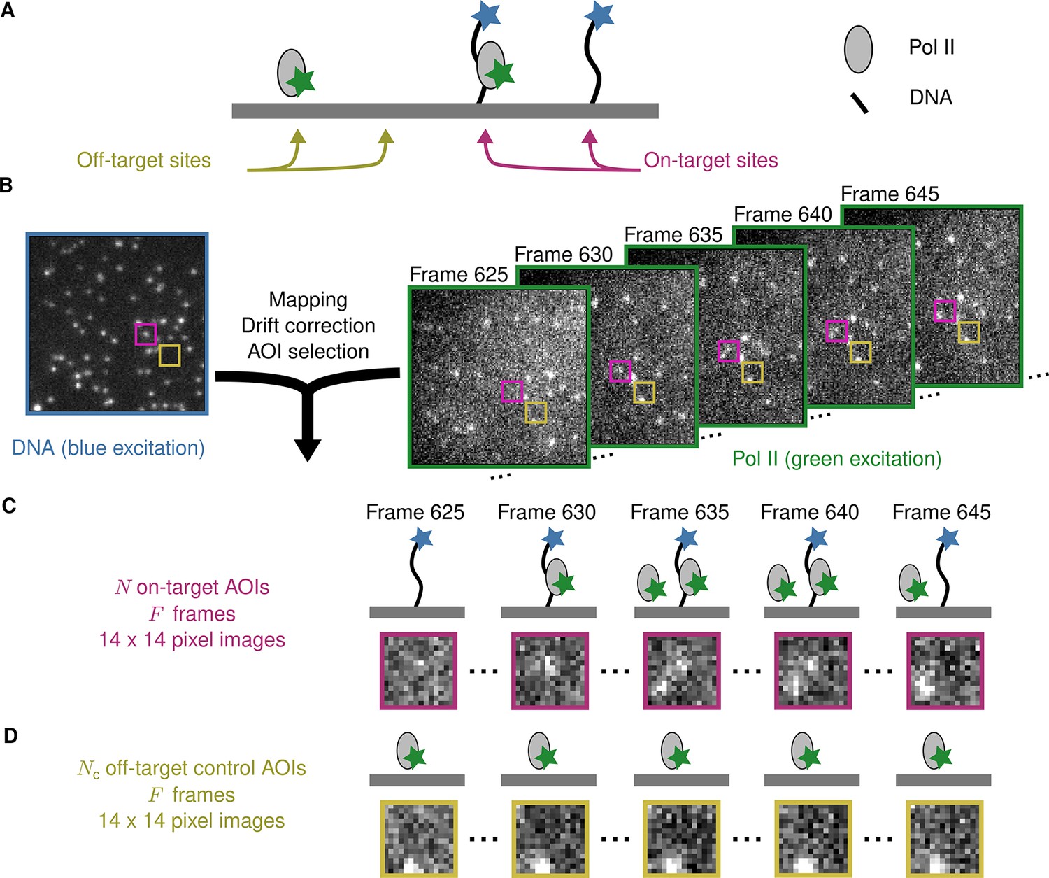
Example CoSMoS experiment.

(A) Experiment schematic. DNA target molecules labeled with a blue-excited fluorescent dye (blue star) are tethered to the microscope slide surface. RNA polymerase II (Pol II) binder molecules labeled with a green-excited dye (green star) are present in solution. (B) Data collection and preprocessing. After collecting a single image with blue excitation to identify the locations of the DNA molecules, a time sequence of Pol II images was collected with green excitation. Preprocessing of the images includes mapping of the corresponding points in target and binder channels, drift correction, and identification of two sets of areas of interest (AOIs). One set corresponds to locations of target molecules (e.g., purple square); the other corresponds to locations where no target is present (e.g., yellow square). (C) On-target data. Data are time sequences of 14 × 14 pixel AOI images centered at each target molecule. Frames show presence of on-target (e.g., frame 630) and off-target (e.g., frame 645) Pol II molecules. (D) Off-target control data. Control data consists of images collected from randomly selected sites at which no target molecule is present. Such sites can be AOIs in which no fluorescent target molecule is visible (e.g., the yellow square in the DNA channel shown in B). Alternatively, control data can be taken from a recording of a separate control sample to which no target molecules were added. Image data in B, C, and D is from Data set A in Table 1.

Effective data analysis is a major challenge in the use of the CoSMoS technique. The basic goal is to acquire information at each time point about whether a binder molecule fluorescence spot is observed at the image position of a target molecule (e.g., whether a colocalized green-dye-labeled RNA polymerase II is observed at the surface location of a blue-dye-labeled DNA spot in Figure 1B). Although CoSMoS images are conceptually simple – they consist only of diffraction-limited fluorescent spots collected in several wavelength channels – efficient analysis of the images is inherently challenging. The number of photons emitted by a single fluorophore is limited by fluorophore photobleaching. Consequently, it is desirable to work at the lowest feasible excitation power in order to maximize the duration of experimental recordings and to efficiently capture relevant reaction events. Achieving higher time resolution divides the number of emitted photons between a larger number of images, so that photon shot noise ordinarily dominates the data statistics. Furthermore, the required concentrations of binder molecules can sometimes create significant background noise (Peng et al., 2018; van Oijen, 2011), even with zero-mode waveguide instruments (Chen et al., 2014). These technical difficulties frequently result in CoSMoS images that have low signal-to-noise ratios (SNR), making discrimination of colocalized fluorescence spots from noise a significant challenge. In addition, there are usually non-specific interactions of the binder molecule with the chamber surface, and these artefacts can give rise to both false positive and false negative spot detection (Friedman and Gelles, 2015). Together, these defects in analyzing spot colocalization interfere with the interpretation of CoSMoS data to measure reaction thermodynamics and kinetics and to infer molecular mechanisms.

Most CoSMoS spot detection methods are based on integrating the binder fluorescence intensity by summing the pixel values in small regions of the image centered on the location of individual target molecules, and then using crossings of an intensity threshold to score binder molecule arrival and departure, e.g., (Friedman and Gelles, 2012; Shcherbakova et al., 2013). However, integration discards data about the spatial distribution of intensity that can (and should) be used to distinguish authentic on-target spots from artefacts caused by noise or off-target binding. More recently, improved methods (Friedman and Gelles, 2015; Smith et al., 2019) were developed that directly analyze TIRF images, using the spatial distribution of binder fluorescence intensity around the target molecule location. All these methods, whether image- or integrated intensity-based, make a binary decision about the presence or absence of a binder spot at the target location. Treating all such binary decisions as equal neglects differences in the confidence of each spot detection decision caused by variations in noise, signal intensity, and non-specific binding. Failure to account for spot confidence decreases the reliability of downstream thermodynamic and kinetic analysis.

In this paper, we describe a qualitatively different Bayesian machine learning method for analysis of CoSMoS data implemented in a computer program, Tapqir (Kazakh: clever, inventive; pronunciation: tap-keer). Tapqir analyzes two-dimensional image data, not integrated intensities. Unlike prior methods, our approach is based on an explicit, global causal model for CoSMoS image formation and uses variational Bayesian inference (Kinz-Thompson et al., 2021; Gelman et al., 2013) to determine the values of model parameters and their associated uncertainties. This model, which we call ‘cosmos’, implements time-independent analysis of single-channel (i.e., one-binder) data sets. The cosmos model is physics-informed and includes realistic shot noise in fluorescent spots and background, camera noise, the size and shape of spots, and the presence of both target-specific and nonspecific binder molecules in the images. Most importantly, instead of yielding a binary spot-/no-spot determination, the algorithm calculates the probability of a target-specific spot being present at each time point and target location. The calculated probability can then be used in subsequent analyses of the molecular thermodynamics and kinetics. Unlike alternative approaches, Tapqir and cosmos do not require subjective threshold settings so they can be used effectively and accurately by non-expert analysts. The program is implemented in the Python-based probabilistic programming language Pyro (Bingham et al., 2019), which enables efficient use of graphics processing unit (GPU)-based hardware for rapid parallel processing of data and facilitates future modifications to the model.

Results

Data analysis pipeline

The initial steps in CoSMoS data analysis involve preprocessing the data set (Figure 1B) to map the spatial relationship between target and binder images, correct for microscope drift (if any) and list the locations of target molecules. Software packages that perform these preprocessing steps are widely available (e.g., Friedman and Gelles, 2015; Smith et al., 2019).

The input into Tapqir consists of the time sequence of images (Figure 1B, right). For colocalization analysis, it is sufficient to consider the image area local to the target molecule. This analyzed area of interest (AOI) needs to be several times the diameter of a diffraction-limited spot to include both the spot and the surrounding background (Figure 1C).

In addition to AOIs centered at target molecules, it is useful to also select negative control AOIs from randomly selected sites at which no target molecule is present (Figure 1B and D). In Tapqir, such off-target control data is analyzed jointly with on-target data and serves to estimate the background level of target-nonspecific binding.

Once provided with the preprocessing data and image sequence, Tapqir computes for each frame of each AOI the probability, $p (s p e c i f i c)$ , that a target-specific fluorescence spot is present. The $p (s p e c i f i c)$ values that are output can then be used to extract information about the kinetics and thermodynamics of the target-binder interaction.

Bayesian image classification analysis

Tapqir calculates $p (s p e c i f i c)$ values using an objective image classification method built on a rigorous Bayesian statistical approach to the CoSMoS image analysis problem. The Bayesian approach has three components. First, we define a probabilistic model of the CoSMoS images. The probabilistic model, cosmos, is a mathematical formalism that describes the AOI images in terms of a set of parameter values. The model is probabilistic in that each parameter is specified to have a probability distribution that defines the likelihood that it can take on particular values. Model parameters describe physically realistic image features such as the characteristic fluorescence spot width. Second, we specify prior distributions for the parameters of the model. These priors embed pre-existing knowledge about the CoSMoS experiment, such as the fact that target-specific spots will be close to the target molecule locations. Third, we infer the values of the model parameters, including $p (s p e c i f i c)$ , using Bayes’ rule (Bishop, 2006; Kinz-Thompson et al., 2021). The cosmos model is ‘time-independent’, meaning that we ignore the time dimension of the recording – the order of the images does not affect the results.

Probabilistic image model and parameters

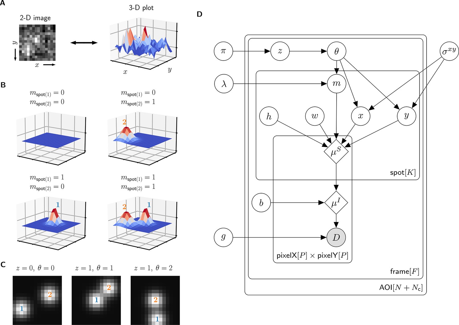
A single AOI image from a CoSMoS data set is a matrix of noisy pixel intensity values. In each image, multiple binder molecule fluorescence spots can be present. Figure 2A shows an example image where two spots are present; one spot is located near the target molecule at the center of the image and another is off-target.

Figure 2 with 2 supplements see all

Download asset Open asset

Depiction of the *cosmos* probabilistic image model and model parameters.

(A) Example AOI image (from Data set A in Table 1). The AOI image is a matrix of 14 × 14 pixel intensities which is shown here as both a 2-D grayscale image and as a 3-D intensity plot. The image contains two spots; one is centered at target location (image center) and the other is located off-target. (B) Examples of four idealized noise-free image representations ( $μ^{I}$ ). Image representations consist of zero, one, or two idealized spots ( $μ^{S}$ ) superimposed on a constant background ( $b$ ). Each fluorescent spot is represented as a 2-D Gaussian parameterized by integrated intensity ( $h$ ), width ( $w$ ), and position ( $x$ , $y$ ). The presence of spots is encoded in the binary spot existence indicator $m$ . (C) Simulated idealized images illustrating different values of the target-specific spot state parameter $z$ and index parameter $θ$ . $θ$ = 0 corresponds to a case when no specifically bound molecule is present ( $z$ = 0); $θ$ = 1 or 2 corresponds to the cases in which specifically bound molecule is present ( $z$ = 1) and corresponds to spot 1 or 2, respectively. (D) Condensed graphical representation of the *cosmos* probabilistic model. Model parameters are depicted as circles and deterministic functions as diamonds. Observed image ( $D$ ) is represented by a shaded circle. Related nodes are connected by edges, with an arrow pointing towards the dependent node (e.g., the shape of each 2-D Gaussian spot $μ^{S}$ depends on spot parameters $m$ , $h$ , $w$ , $x$ , and $y$ ). Plates (rounded rectangles) contain entities that are repeated for the number of instances displayed at the bottom-right corner: number of total AOIs ( $N + N_{c}$ ), frame count ( $F$ ), and maximum number of spots in a single image ( $K$ = 2). Parameters outside of the plates are global quantities that apply to all frames of all AOIs. A more complete version of the graphical model specifying the relevant probability distributions is given in Figure 2—figure supplement 1.

The probabilistic model mathematically generates images $D$ as follows. We construct a noise-free AOI image $μ^{I}$ as a constant average background intensity $b$ summed with fluorescence spots modeled as 2-D Gaussians $μ^{S}$ , which accurately approximate the microscope point spread function (Zhang et al., 2007; Figure 2B). Each 2-D Gaussian is described by parameters integrated intensity $h$ , width $w$ , and position ( $x$ , $y$ ). We define $K$ as the maximum number of spots that can be present in a single AOI image. For the data we typically encounter, $K$ = 2 is sufficient. Since the spots may be present or not in a particular image, we define the $K$ = 2 binary indicators $m_{s p o t (1)}$ and $m_{s p o t (2)}$ . Each indicator can take a value of either 0 denoting spot absence or 1 denoting spot presence.

The resulting mixture model has four possible combinations for $m_{s p o t (1)}$ and $m_{s p o t (2)}$ : (1) a no-spot image that contains only background (Figure 2B, top left), (2) a single-spot image that contains the first binder molecule spot superimposed on background (Figure 2B, bottom left), (3) a single-spot image that contains the second binder molecule spot superimposed on background (Figure 2B, top right), and (4) a two-spot image that contains both binder molecule spots superimposed on background (Figure 2B, bottom right).

Among the spots that are present in an AOI image, by assumption at most only one can be target-specific. We use a state parameter $z$ to indicate target-specific spot absence ( $z$ = 0) or presence ( $z$ = 1) in an AOI image. We also introduce an index parameter $θ$ that identifies which of the spots is the target-specific spot when it is present ( $z$ = 1) (e.g., Figure 2C, middle and right have $θ$ = 1 and $θ$ = 2, respectively) and equals zero when it is absent ( $z$ = 0) (e.g., Figure 2C, left). Since the off-target control AOIs by definition contain only non-specific binding, $z$ = 0 and $θ$ = 0 for all off-target AOIs.

Finally, to construct realistic noisy AOI images $D$ from the noise-free images $μ^{I}$ , the model adds intensity-dependent noise to each pixel. For cameras that use charge-coupled device (CCD) or electron-multiplier CCD (EMCCD) sensors, each measured pixel intensity in a single-molecule fluorescence image has a noise contribution from photon counting (shot noise) and can also contain additional noise arising from electronic amplification (van Vliet et al., 1998). The result is a characteristic linear relationship between the noise variance and mean intensity with slope defining the gain $g$ . This relationship is used to compute the random pixel noise values (see Materials and methods).

The resulting probabilistic image model can be interpreted as a generative process that produces the observed image data $D$ . A graphical representation of the probabilistic relationships in the model is shown in Figure 2D. A complete description of the model is given in Materials and methods and Figure 2—figure supplement 1.

Parameter prior distributions

Specifying prior probability distributions for model parameters is essential for Bayesian analysis and allows us to incorporate pre-existing knowledge about the experimental design. For most model parameters, there is no strong prior information so we use uninformative prior distributions (see Materials and methods). However, we have strong expectations for the positions of specific and non-specific binder molecules that can be expressed as prior distributions and used effectively to discriminate between the two. Non-specific binding can occur anywhere on the surface with equal probability and thus has a uniform prior distribution across the AOI image. Target-specific binding, on the other hand, is colocalized with the target molecule and thus has a prior distribution peaked at the AOI center (Figure 2—figure supplement 2). The width of this peak, proximity parameter $σ^{x y}$ , depends on multiple features of the experiment such as the spot localization accuracy and the mapping accuracy between target and binder imaging channels. Prior distributions for parameters $θ$ and $m$ are defined in terms of the average number of target-specific and target non-specific spots per AOI image, $π$ and $λ$ , respectively. To facilitate convenient use of the algorithm, it is not necessary to pre-specify values of $σ^{x y}$ , $π$ , and $λ$ . Instead, values of these parameters appropriate to a given data set are calculated automatically using a hierarchical Bayesian analysis (see Materials and methods; for hierarchical modeling see Chapter 5 of Gelman et al., 2013).

Bayesian inference and implementation

Tapqir calculates posterior distributions of model parameters conditioned on the observed data by using Bayes’ theorem. In particular, Tapqir approximates posterior distributions using a variational inference approach implemented in Pyro (Bingham et al., 2019). Complete details of the implementation are given in Materials and methods.

Tapqir analysis

In initial tests, we used Tapqir to analyze simulated CoSMoS image data with a comparatively high SNR of 3.76 as well as data from the experiment shown in Figure 1B–D, which has a lower SNR of 1.61. The simulated data were generated using the same cosmos model (Figure 2D) that was used for analysis. Tapqir correctly detects fluorescent spots in both simulated and experimental images (compare ‘AOI images’ and ‘Spot-detection’ rows in Figure 3). The program precisely calculates the position ( $x$ , $y$ ), intensity ( $h$ ), and width ( $w$ ) for each spot and also determines the background intensity ( $b$ ) for each image without requiring a separate analysis. These parameters confirm the desired behavior of the model and could be used in further calculations. However, the most important output of the analysis is assessment of the presence of target-specific binding. For each AOI image, we calculate $p (s p e c i f i c) \equiv p (z = 1)$ (Figure 3, green), the probability that any target-specific spot is present. Spots determined as likely target-specific ( $p (s p e c i f i c)$ > 0.5) are represented as filled circles in the spot detection row of Figure 3. For a particular spot to have high $p (s p e c i f i c)$ , it must have a high spot probability and be colocalized with the target molecule at the center of the AOI (Figure 3—figure supplement 1).

Figure 3 with 4 supplements see all

Download asset Open asset

Tapqir analysis and inferred model parameters.

(**A,B**) Tapqir was applied to simulated data (lamda0.5 parameter set in Supplementary file 1) (A) and to experimental data (Data set A in Table 1) (B). (A) and (B) each show a short extract from a single target location in the data set. The first row shows AOI images for the subset of frames indicated by gray shaded stripes in the plots; image contrast and offset settings are consistent within each panel. The second row shows the locations of spots determined by Tapqir. Spot numbers 1 (blue) and 2 (orange) are assigned arbitrarily and may change from fame to frame. For clarity, only data for spots with a spot probability $p (m = 1)$ > 0.5 are shown. Spots predicted to be target-specific ( $p (θ = k)$ > 0.5 for spot $k$ ) are shown as filled circles. The topmost graphs (green) show the calculated probability that a target-specific spot is present ( $p (s p e c i f i c)$ ) in each frame. Below are the calculated spot intensities ( $h$ ), spot widths ( $w$ ), and locations ( $x$ , $y$ ) for spot 1 (blue) and spot 2 (orange), and the AOI background intensities ( $b$ ). Again, for clarity data are only shown for likely spots ( $p (m = 1)$ > 0.5). Error bars: 95% CI (credible interval) estimated from a sample size of 500. Some error bars are smaller than the points and thus not visible.

Tapqir robustly fits experimental data sets with different characteristics

Next, we evaluated how well the model fits data sets encompassing a range of characteristics found in typical CoSMoS experiments. We analyzed four experimental data sets with varying SNR, frequency of target-specific spots, and frequencies of non-specific spots (Table 1). We then sampled AOI images from the posterior distributions of parameters (a method known as posterior predictive checking Gelman et al., 2013). These posterior predictive simulations accurately reproduce the experimental AOI appearances, recapitulating the noise characteristics and the numbers, intensities, shapes, and locations of spots (Figure 3—figure supplement 2, images). The distributions of pixel intensities across the AOI are also closely reproduced (Figure 3—figure supplement 2, histograms) confirming that the noise model is accurate. Taken together, these results confirm that the model is rich enough to accurately capture the full range of image characteristics from CoSMoS data sets taken over different experimental conditions. Importantly, all the results on different experimental data sets were obtained using the same model (Figure 2D) and the same priors (Materials and methods). No tuning of the algorithm or prior measurement of data-set-specific properties was needed to achieve good fits for all data sets.

Table 1

Experimental data sets.

Data set size^a	SNR	π [95% CI]	λ [95% CI]	g [95% CI]	σ^xy [95% CI]	Compute time
Data set A: Binder, SNAP_f-tagged S. cerevisiae RNA polymerase II labeled with DY549; Target, transcription template DNA containing 5× Gal4 upstream activating sequences and CYC1 core promoter; Conditions, yeast nuclear extract supplemented with Gal4-VP16 activator and NTPs. From Rosen et al., 2020.
$N$ = 331, $N_{c}$ = 526, $F$ = 790	1.61	0.0951 [0.0936, 0.0966]	0.2943 [0.2924, 0.2963]	6.645 [6.643, 6.647]	0.577 [0.573, 0.580]	7 h 40 m^b 3 h 50 m^c
Data set B: Binder, 0.1 nM E. coli σ⁵⁴ RNA polymerase labeled with Cy3; Target, 852 bp DNA containing the glnALG promoter; Conditions, physiological buffer, no NTPs. From (Fig. 1E) of Friedman et al., 2013.
$N$ = 102, $N_{c}$ = 127, $F$ = 4407	3.77	0.0846 [0.0835, 0.0857]	0.1575 [0.1569, 0.1583]	11.861 [11.856, 11.865]	0.476 [0.474, 0.479]	7 h 40 m^b
Data set C: Binder, 0.4 nM E. coli σ⁵⁴ RNA polymerase labeled with Cy3; Target, 3,591 bp DNA containing the glnALG promoter; Conditions, physiological buffer, no NTPs. From (Fig. 3D) of Friedman et al., 2013.
$N$ = 122, $N_{c}$ = 157, $F$ = 3855	4.23	0.0267 [0.0262, 0.0273]	0.0876 [0.0869, 0.0883]	16.777 [16.773, 16.782]	0.404 [0.399, 0.408]	9 h 15 m^b
Data set D: Binder, 0.15 nM E. coli Cy3-GreB; Target, reconstituted backtracked EC-6 E. coli transcription elongation complex; Conditions, physiological buffer, no NTPs. Randomly selected subset of data set from Tetone et al., 2017.
$N$ = 200, $N_{c}$ = 200, $F$ = 5622	3.06	0.0038 [0.0036, 0.0039]	0.0437 [0.0434, 0.0440]	18.727 [18.724, 18.731]	0.451 [0.438, 0.463]	11 h^b

*N - number of on-target AOIs, N_c - number of control off-target AOIs, F - number of frames.
^bUnattended calculation time on an AMD Ryzen Threadripper 2990WX with an Nvidia GeForce RTX 2080Ti GPU using CUDA version 11.5.
^cUnattended calculation time on an Intel Xeon CPU with an Nvidia Tesla V100-SXM2-16GB GPU using CUDA version 11.2 in a Google Colab Pro account.

Tapqir accuracy on simulated data with known global parameter values

Next, we evaluated Tapqir’s ability to reliably infer the values of global model parameters. To accomplish this, we generated simulated data sets using a wide range of randomized parameter values and then fit the simulated data to the model (Supplementary file 2). Fit results show that global model parameters (i.e., average specific spot probability $π$ , nonspecific binding density $λ$ , proximity $σ^{x y}$ , and gain $g$ ; see Figure 2D) are close to the simulated values (Figure 3—figure supplement 3 and Supplementary file 2). This suggests that CoSMoS data contains enough information to reliably infer global model parameters and that the model is not obviously overparameterized.

Tapqir classification accuracy

Having tested the basic function of the algorithm, we next turned to the key question of how accurately Tapqir can detect target-specific spots in data sets of increasing difficulty.

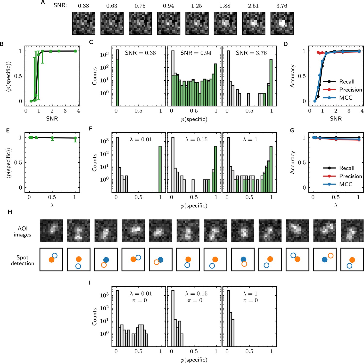
We first examined the accuracy of target-specific spot detection in simulated data sets with decreasing SNR (Supplementary file 3). By eye, spots can be readily discerned at SNR >1 but cannot be clearly seen at SNR <1 (Figure 4A). Tapqir gives similar or better performance: if an image contains a target-specific spot, Tapqir correctly assigns it a target-specific spot probability $p (s p e c i f i c)$ that is on average close to one as long as SNR is adequate (i.e., SNR >1) (Figure 4B). In contrast, mean $p (s p e c i f i c)$ sharply decreases at SNR <1, consistent with the subjective impression that no spot is recognized under those conditions. In particular, images that contain a target-specific spot are almost always assigned a high $p (s p e c i f i c)$ for high SNR data and almost always assigned low $p (s p e c i f i c)$ for low SNR data (Figure 4C, green). At marginal SNR ≈ 1, these images are assigned a broad distribution of $p (s p e c i f i c)$ values, accurately reflecting the uncertainty in classifying such data. Just as importantly, images with no target-specific spot are almost always assigned $p (s p e c i f i c)$ < 0.5, correctly reflecting the absence of the spot (Figure 4C, gray).

Figure 4 with 1 supplement see all

Download asset Open asset

Tapqir performance on simulated data with different SNRs or different non-specific binding densities.

(**A–D**) Analysis of simulated data over a range of SNR. SNR was varied in the simulations by changing spot intensity $h$ while keeping other parameters constant (Supplementary file 3). (A) Example images showing the appearance of the same target-specific spot simulated with increasing SNR. (B) Mean of Tapqir-calculated target-specific spot probability $p (s p e c i f i c)$ (with 95% CI; see Materials and methods) for the subset of images where target-specific spots are known to be present. (C) Histograms of $p (s p e c i f i c)$ for selected simulations with SNR indicated. Data are shown as stacked bars for images known to have (green, 15%) or not have (gray, 85%) target-specific spots. Count is zero for bins where bars are not shown. (D) Accuracy of Tapqir image classification with respect to presence/absence of a target-specific spot. Accuracy was assessed by MCC, recall, and precision (see Results and Materials and methods sections). (**E–G**) Same as in (**B–D**) but for the data simulated over a range of non-specific binding densities $λ$ at fixed SNR = 3.76 (Supplementary file 1). (H) Spot recognition in AOI images containing closely spaced target-specific and non-specific spots. Images were selected from the $λ$ = 1 data set in (**E–G**). AOI images and spot detection are plotted as in Figure 3, with spot numbers 1 (blue) and 2 (orange) assigned arbitrarily and spots predicted to be target-specific shown as filled circles. (I) Same as in (C) but for the data simulated over a range of non-specific binding densities $λ$ with no target-specific binding ( $π$ = 0) (Supplementary file 4).

Ideally, we want to correctly identify target-specific binding when it occurs but also to avoid incorrectly identifying target-specific binding when it does not occur. To quantify Tapqir’s classification accuracy, we next examined binary image classification statistics. Binary classification predictions were obtained by thresholding $p (s p e c i f i c)$ at 0.5. We then calculated two complementary statistics: recall and precision (Fawcett, 2006; Figure 4D; see Materials and methods). Recall is defined as the fraction of true target-specific spots that are correctly predicted. Recall is high at high SNR and decreases at lower SNR. Recall is a binary analog of the mean $p (s p e c i f i c)$ for the subset of images containing target-specific spots; as expected the two quantities have similar dependencies on SNR (compare Figure 4B and D, black). Precision is the fraction of predicted target-specific spots that are correctly predicted. Precision is near one at all SNR values tested (Figure 4D, red); this shows that the algorithm rarely misclassifies an image as containing a target-specific spot when none is present.

In order to quantify the effects of both correctly and incorrectly classified images in a single statistic, we used the binary classification predictions to calculate the Matthews Correlation Coefficient (MCC) (Matthews, 1975; see Materials and methods). The MCC is equivalent to the Pearson correlation coefficient between the predicted and true classifications, giving 1 for a perfect match, 0 for a random match, and –1 for complete disagreement. The MCC results (Figure 4D, blue) suggest that the overall performance of Tapqir is excellent at SNR ≥ 1: the program rarely misses target-specific spots that are in reality present and rarely falsely reports a target-specific spot when none is present.

The analyses of Figure 4B–D examined Tapqir performance on data in which the rate of target-nonspecific binding is moderate ( $λ$ = 0.15 non-specific spots per AOI image on average). We next examined the effects of increasing the non-specific rate. In particular, we used simulated data (Supplementary file 1) with high SNR = 3.76 to test the classification accuracy of Tapqir at different non-specific binding densities up to $λ$ = 1, a value considerably higher than typical of usable experimental data (the experimental data sets in Table 1 have $λ$ ranging from 0.04 to 0.30). In analysis of these data sets, a few images with target-specific spots are misclassified as not having a specific spot ( $p (s p e c i f i c)$ near zero) or as being ambiguous ( $p (s p e c i f i c)$ near 0.5) (Figure 4F, green bars), and a few images with target-nonspecific spots are misclassified as having specific spot ( $p (s p e c i f i c)$ near or above 0.5) (Figure 4F, gray bars), but these misclassifications only occurred at the unrealistically high $λ$ value. Even in the simulation with this highest $λ$ value, Tapqir accurately identified target-specific spots (Figure 4E and F) and returned excellent binary classification statistics (Figure 4G).

A weakness of some existing image-based CoSMoS spot discrimination methods is that target-nonspecific binding adjacent to a target-specific spot can interfere with correctly identifying the latter as target-specific. The very high recall values obtained at $λ$ = 1 (Figure 4G) confirm that there are few such misidentifications by Tapqir even at high non-specific binding densities. This good performance is likely facilitated by the feature of the Tapqir model that explicitly includes the possibility that both a specifically and a non-specifically bound spot may occur simultaneously in the same AOI. Consistent with this interpretation, we see effective detection of the specific and non-specific spots even in example AOIs in which the two spots are so closely spaced that they are not completely resolved (Figure 4H). In contrast, tests of existing CoSMoS image classification methods show that images with target-nonspecific spots are prone to misclassification. As discussed previously (Friedman and Gelles, 2015), methods based on thresholding of integrated AOI intensities are prone to incorrectly classify target-nonspecific spots as target-specific. Conversely, an existing ‘spot-picker’ method based on empirical binary classification of 2-D AOI images (Friedman and Gelles, 2015) is much more likely than Tapqir to fail to detect target specific spots when there is a nearby non-specific spot (Figure 4—figure supplement 1). This contributes to the superior overall performance we see for Tapqir vs. spot-picker on the $λ$ = 1 data set (recall 0.993 vs 0.919; precision 0.943 vs 0.873; MCC 0.961 vs 0.874).

To further evaluate whether Tapqir is prone to misidentifying target-nonspecific spots as specific, we simulated data sets with no target-specific binding at both low and high non-specific binding densities (Supplementary file 4). Analysis of such data (Figure 4I) shows that no target-specific binding (i.e., $p (s p e c i f i c)$ > 0.6) was detected even under the highest non-specific binding density, demonstrating that Tapqir is robust to false-positive target-specific spot detection even under these extreme conditions.

Since target-nonspecific spots are built into the cosmos model, there is no need to choose excessively small AOIs in an attempt to exclude non-specific spots from analysis. We found that reducing AOI size (from 14 × 14 to 6 x 6 pixels) did not appreciably affect analysis accuracy on simulated data, when the width ( $w$ ) of the spots was equal to 1.4 pixels (Table 2). In analysis of experimental data, smaller AOI sizes caused occasional changes in calculated $p (s p e c i f i c)$ values reflecting apparent missed detection of a few spots (Figure 3—figure supplement 4). Out of caution, we therefore used 14 × 14 pixel AOIs routinely, even though the larger AOIs somewhat reduced computation speed (Table 2 and Figure 3—figure supplement 4).

Table 2

The effect of AOI size on classification accuracy*.

AOI dimension^†, P (pixels)	MCC	Compute time^‡
14	0.951	2 h 10 m
10	0.948	1 h 25 m
6	0.939	1 h 20 m

*

Tapqir was applied to the same simulated data set (height1000 parameter set in Supplementary file 3; SNR = 1.25) using different AOI sizes.
†

The width ( $w$ ) of the simulated spots (one standard deviation of the 2-D Gaussian) is equal to 1.4 pixels.
‡

Unattended calculation time on an AMD Ryzen Threadripper 2990WX with an Nvidia GeForce RTX 2080Ti GPU using CUDA version 11.5.

Kinetic and thermodynamic analysis of molecular interactions

The most widespread application of CoSMoS experiments is to measure rate and equilibrium constants for the binding interaction of the target and binder molecules being studied. We next tested whether these constants can be accurately determined using Tapqir-calculated posterior predictions.

We first simulated CoSMoS data sets (Supplementary file 5) that reproduced the behavior of a one-step association/dissociation reaction mechanism (Figure 5A and B, blue). Simulated data were analyzed with Tapqir yielding $p (s p e c i f i c)$ values for each frame (e.g., Figure 5B, green). We wanted to estimate rate constants using the full information contained in the $p (s p e c i f i c)$ probabilities, so we did not threshold $p (s p e c i f i c)$ for this analysis. Instead, from each single-AOI $p (s p e c i f i c)$ time record we constructed a family of binary time records (Figure 5B, black) by Monte Carlo sampling according to the $p (s p e c i f i c)$ time series. Each family member has well-defined target-specific binder-present and binder-absent intervals $Δ t_{o n}$ and $Δ t_{o f f}$ , respectively. Each of these time records was then analyzed with a two-state hidden Markov model (HMM) (see Materials and methods), producing a distribution of inferred rate constants from which we calculated mean values and their uncertainties (Figure 5C and D). Comparison of the simulated and inferred values shows that both $k_{o n}$ and $k_{o f f}$ rate constants are accurate within 30% at nonspecific binding densities typical of experimental data ( $λ$ ≤ 0.5). At higher nonspecific binding densities, rare interruptions caused by false-positive and false-negative spot detection shorten $Δ t_{o n}$ and $Δ t_{o f f}$ distributions, leading to moderate systematic overestimation of the association and dissociation rate constants.

Figure 5

Download asset Open asset

Tapqir analysis of association/dissociation kinetics and thermodynamics.

(A) Chemical scheme for a one-step association/dissociation reaction at equilibrium with pseudo-first-order binding and dissociation rate constants $k_{o n}$ and $k_{o f f}$ , respectively. (B) A simulation of the reaction in (A) and scheme for kinetic analysis of the simulated data with Tapqir. The simulation used SNR = 3.76, $k_{o n}$ = 0.02 s⁻¹, $k_{o f f}$ = 0.2 s⁻¹, and a high target-nonspecific binding frequency $λ$ = 1 (Supplementary file 5, data set kon0.02lamda1). Full dataset consists of 100 AOI locations and 1,000 frames each for on-target data and off-target control data. Shown is a short extract of on-target data from a single AOI location in the simulation. Plots show simulated presence/absence of the target-specific spot (blue) and Tapqir-calculated estimate of corresponding target-specific spot probability $p (s p e c i f i c)$ (green). Two thousand binary traces (e.g., black records) were sampled from the $p (s p e c i f i c)$ posterior distribution and used to infer $k_{o n}$ and $k_{o f f}$ using a two-state hidden Markov model (HMM) (see Materials and methods). Each sample trace contains well-defined time intervals corresponding to target-specific spot presence and absence (e.g., $Δ t_{o n}$ and $Δ t_{o f f}$ ). (**C,D,E**) Kinetic and equilibrium constants from simulations (Supplementary file 5) using a range of $k_{o n}$ values and target-nonspecific spot frequencies $λ$ , with constant $k_{o f f}$ = 0.2 s⁻¹. (C) Values of $k_{o n}$ used in simulations (blue) and mean values (and 95% CIs, black) inferred by HMM analysis from the 2000 posterior samples. Some error bars are smaller than the points and thus not visible. (D) Same as (C) but for $k_{o f f}$ . (E) Binding equilibrium constants $K_{e q} = k_{o n} / k_{o f f}$ used in simulation (blue) and inferred from Tapqir-calculated π as $K_{e q} = π / (1 - π)$ (black).

From the same simulated data, we calculated the equilibrium constant $K_{e q}$ and its uncertainty. This calculation does not require a time-dependent model and can be obtained directly from the posterior distribution of the average specific-binding probability $π$ . The estimated equilibrium constants are highly accurate even at excessively high values of $λ$ (Figure 5E). The high accuracy results from the fact that equilibrium constant measurements are in general much less affected than kinetic measurements by occasional false positives and false negatives in spot detection.

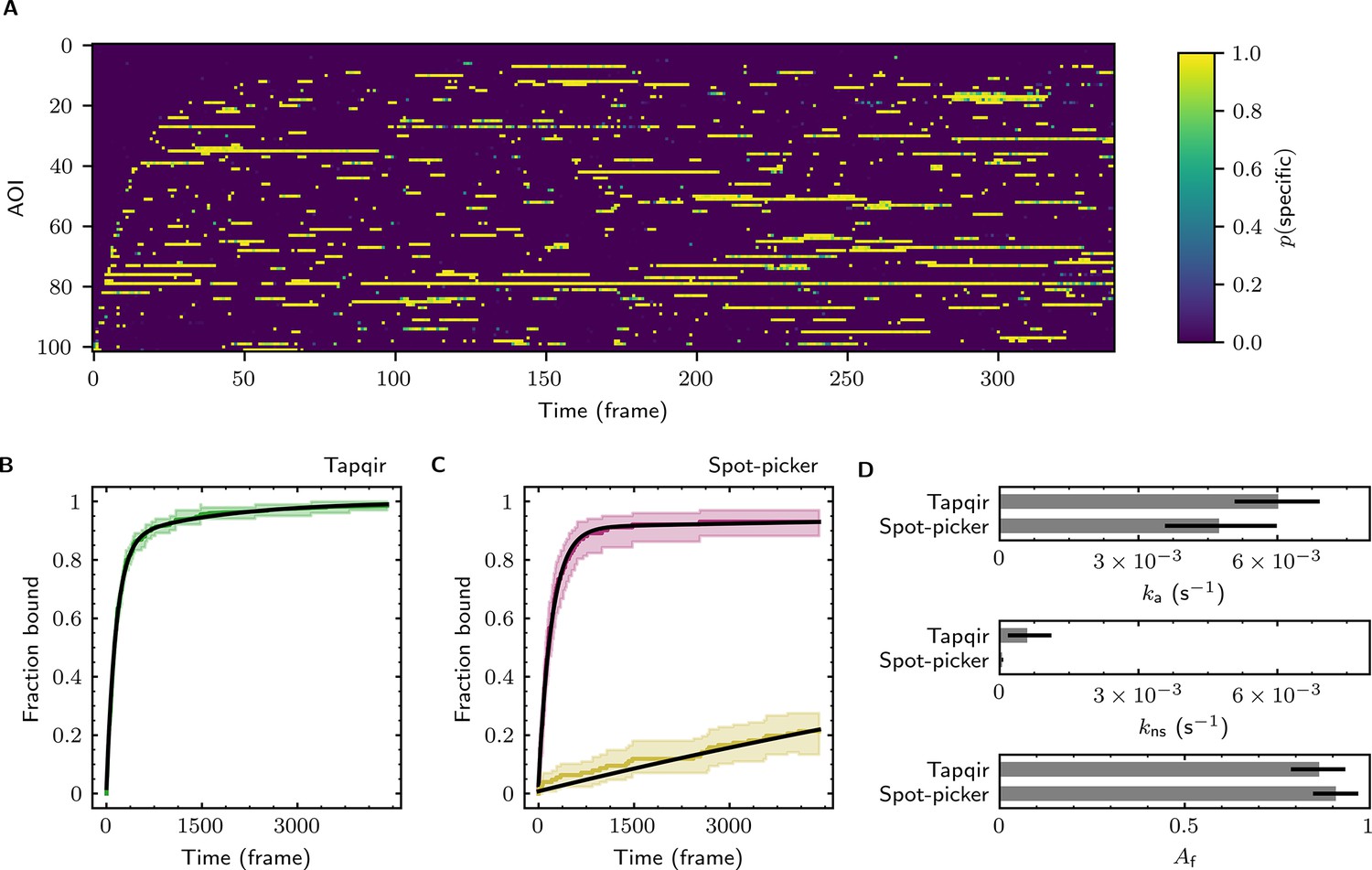
The forgoing analysis shows that Tapqir can accurately recover kinetic and thermodynamic constants from simulated CoSMoS data. However, experimental CoSMoS data sets can be more diverse. In addition to having different SNR and non-specific binding frequency values, they also may have non-idealities in spot shape (caused by optical aberrations) and in noise (caused by molecular diffusion in and out of the TIRF evanescent field). In order to see if Tapqir analysis is robust to these and other properties of real experimental data, we analyzed several CoSMoS data sets taken from different experimental projects. Analysis of each data set took a few hours of computation time on a GPU-equipped desktop computer or cloud computing service (Table 1). We first visualized the results as probabilistic rastergrams (Figure 6A, Figure 6—figure supplement 1A, Figure 6—figure supplement 2A, and Figure 6—figure supplement 3A), in which each horizontal line represents the time record from a single AOI. Unlike the binary spot/no-spot rastergrams in previous studies (e.g., Friedman et al., 2013; Rosen et al., 2020) we plotted the Tapqir-calculated spot probability $p (s p e c i f i c)$ using a color scale. This representation allows a more nuanced understanding of the data. For example, Figure 6A reveals that while the long-duration spot detection events typically are assigned a high probability (yellow), some of the shortest duration events have an intermediate $p (s p e c i f i c)$ (green) indicating that the assignment of these as target-specific is uncertain.

Figure 6 with 3 supplements see all

Download asset Open asset

Extraction of target-binder association kinetics from example experimental data.

Data are from Data set B (SNR = 3.77, $λ$ = 0.1575; see Table 1). (A) Probabilistic rastergram representation of Tapqir-calculated target-specific spot probabilities $p (s p e c i f i c)$ (color scale). AOIs were ordered by decreasing times-to-first-binding. For clarity, only every thirteenth frame is plotted. (B) Time-to-first-binding distribution using Tapqir. Plot shows the cumulative fraction of AOIs that exhibited one or more target-specific binding events by the indicated frame number (green) and fit curve (black). Shading indicates uncertainty. (C) Time-to-first-binding distribution using an empirical spot-picker method Friedman et al., 2013. The spot-picker method jointly fits first spots observed in off-target control AOIs (yellow) and in on-target AOIs (purple) yielding fit curves (black). (D) Values of kinetic parameters $k_{a}$ , $k_{n s}$ , and $A_{f}$ (see text) derived from fits in (B) and (C). Uncertainties reported in (**B, C, D**) represent 95% credible intervals for Tapqir and 95% confidence intervals for spot-picker (see Materials and methods).

To demonstrate the utility of Tapqir for kinetic analysis of real experimental data, we measured binder association rate constants in previously published experimental data sets (Table 1). We employed our previous strategy (Friedman and Gelles, 2012; Friedman and Gelles, 2015) of analyzing the duration of the binder-absent intervals that preceded the first binding event. Such time-to-first binding analysis improves the accuracy of association rate constant estimates relative to those obtained by analyzing all $Δ t_{o f f}$ values by minimizing the effects of target molecules occupied by photobleached binders, dye blinking and false negative dropouts that occur within a continuous binder dwell interval. To perform a time-to-first-binding analysis using Tapqir, we used the posterior sampling method (as in Figure 5B, black records) to determine the initial $Δ t_{o f f}$ in each AOI record. These data were fit to a kinetic model (Friedman and Gelles, 2012; Friedman and Gelles, 2015) in which only a fraction of target molecules $A_{f}$ were binding competent and which includes both exponential target-specific association with rate constant $k_{a}$ , as well as exponential non-specific association with rate constant $k_{n s}$ (Figure 6B, Figure 6—figure supplement 1B, Figure 6—figure supplement 2B, and Figure 6—figure supplement 3B). The Tapqir-derived fits showed excellent agreement with the kinetic model.

To further assess the utility of the Tapqir method, we used experimental data sets and compared the Tapqir association kinetics results with those from the previously published empirical binary ‘spot-picker’ method (Friedman and Gelles, 2015; Figure 6C, Figure 6—figure supplement 1C, Figure 6—figure supplement 2C, and Figure 6—figure supplement 3C). The values of the association rate constant $k_{a}$ obtained using these two methods are in good agreement with each other (Figure 6D, Figure 6—figure supplement 1D, Figure 6—figure supplement 2D, and Figure 6—figure supplement 3D). We emphasize that while Tapqir is fully objective, achieving these results with the spot-picker method required optimization by subjective adjustment of spot detection thresholds. We noted some differences between the two methods in the non-specific association rate constants $k_{n s}$ . Differences are expected because these parameters are defined differently in the different non-specific binding models used in Tapqir and spot-picker (see Materials and methods).

Discussion

A broad range of physical processes contribute to the formation of CoSMoS images. These include camera and photon noise, target-specific and non-specific binding, and time- and position-dependent variability in fluorophore imaging and image background. Unlike prior CoSMoS analysis methods, Tapqir considers these aspects of imaging in a single, holistic model. This cosmos model explicitly includes the uncertainties due to photon noise, camera gain, and spatial variability in intensity offset. The model also includes the possibility of multiple binder molecule fluorescence spots being present in the vicinity of the target, including both target-specific binding and target-nonspecific interactions of binder molecules with the coverslip surface. This explicit modeling of target-nonspecific spots makes it possible to include off-target control data as a part of the experimental data set. Similarly, all AOIs and frames in the data set are simultaneously fit to the global model in a way that allows for realistic frame-to-frame and AOI-to-AOI variability in image formation caused by variations in laser intensity, fluctuations in background, and other non-idealities. The global analysis based on a single, unified model enables the final results (e.g., kinetic and thermodynamic parameters) to be estimated in a way that is cognizant of the known sources of uncertainty in the data.

Previous approaches to CoSMoS data analysis, including our spot-picker method (Friedman and Gelles, 2015), did not employ a holistic modeling approach and instead relied on a multi-step process that includes a separate binary classification step. These prior methods require subjective setting of classification thresholds. Because they are not fully objective, such methods cannot reliably account for uncertainties in spot classification, which compromises error estimates in the analysis pipeline downstream of spot classification. One recent approach (Smith et al., 2019; Smith et al., 2015), which like spot-picker and Tapqir analyzes 2-D images instead of integrated intensities, used a Bayesian kinetic analysis but a frequentist hypothesis test (a generalized likelihood ratio test) for spot detection. The frequentist method lacks a key advantage of Tapqir’s model-based Bayesian approach that here enables prediction of target-specific spot presence probabilities $p (s p e c i f i c)$ for each image, rather than a binary ‘spot/no spot’ classification. In general, previous approaches in essence assume that spot classifications are correct, and thus the uncertainties in the derived molecular properties (e.g., equilibrium constants) are systematically underestimated because the errors in spot classification, which can be large, are not accounted for. By performing a probabilistic spot classification, Tapqir enables reliable inference of molecular properties, such as thermodynamic and kinetic parameters, and allows statistically well-justified estimation of parameter uncertainties. This more inclusive error estimation likely accounts for the generally larger kinetic parameter error bars obtained from Tapqir compared to those from the existing spot-picker analysis method (Figure 6, Figure 6—figure supplement 1, Figure 6—figure supplement 2, and Figure 6—figure supplement 3). Even though existing analysis methods take advantage of subjective tuning by a human analyst, our comparisons show that Tapqir performs at least comparably to (Figure 6, Figure 6—figure supplement 1, Figure 6—figure supplement 2, and Figure 6—figure supplement 3) and under some conditions much better than (Figure 4—figure supplement 1) the existing spot-picker method.

The Tapqir cosmos model includes parameters of mechanistic interest, such as the average probability of target-specific binding, as well as ‘nuisance’ parameters that are not of primary interest but nevertheless essential for image modeling. In previous image-based methods for CoSMoS analysis (e.g., Friedman and Gelles, 2015; Smith et al., 2019), nuisance parameters were either measured in separate experiments (e.g., gain was determined from calibration data), set heuristically (e.g., a subjective choice of user-set thresholds for spot intensity and proximity in colocalization detection), or determined at a separate analysis step (e.g., rate of non-specific binding). In contrast, Tapqir directly learns parameters from the full set of experimental data, thus eliminating the need for additional experiments, subjective adjustment of tuning parameters, and post-processing steps.

Bayesian analysis has been used previously to analyze data from single-molecule microscopy experiments (e.g., Kinz-Thompson et al., 2021 and references cited therein). A key feature of Bayesian analysis is that the extent of prior knowledge of all model parameters is explicitly incorporated. Where appropriate, cosmos uses relatively uninformative priors that only weakly specify information about the value of the corresponding parameters. In these cases, cosmos mostly infers parameter values from the data. In contrast, some priors are more informative. For example, binder molecule spots near the target molecule are more likely to be target-specific rather than target-nonspecific, so we use this known feature of the experiment by encoding the likely position of target-specific binding as a data-based prior. This tactic effectively enables probabilistic classification of spots as either target-specific or target-nonspecific, which would be difficult using other inference methodologies, while still accommodating data sets with different accuracies of mapping between binder and target channels.

Tapqir is implemented in Pyro, a Python-based probabilistic programming language (PPL) (Bingham et al., 2019). Probabilistic programming is a relatively new paradigm in which probabilistic models are expressed in a high-level language that allows easy formulation, modification, and automated inference (van de Meent et al., 2018). In this work we focused on developing an image model for colocalization detection in a relatively simple binder-target single-molecule experiment. However, Tapqir can be used with more complex models. For example, the cosmos model could be naturally extended to multi-state and multi-color analysis. Furthermore, with the development of more efficient sequential hidden Markov modeling algorithms (Särkkä and García-Fernández, 2019; Obermeyer et al., 2019b) Tapqir can potentially be extended to directly incorporate kinetic processes, allowing direct inference of kinetic mechanisms and rate constants.

Tapqir is free, open-source software. Tapqir is available at https://github.com/gelles-brandeis/tapqir. The results presented here were obtained using release 1.0 of the program (https://github.com/gelles-brandeis/tapqir/releases/tag/v1.0). The Tapqir documentation, which contains tutorials on program use, is at https://tapqir.readthedocs.io/en/stable/. Source data including Figures, Figure supplements, Supplementary files, manuscript text, and the scripts and data used to generate them are available at https://github.com/ordabayevy/tapqir-overleaf.

Materials and methods

Notation

Request a detailed protocol

In the Materials and methods section, we adopt a mathematical notation for multi-dimensional arrays from the field of machine learning (Chiang et al., 2021). The notation uses named axes and incorporates implicit broadcasting of arrays when their shapes are different.

Extracting image data

Request a detailed protocol

Raw input data into Tapqir consists of (1) binder channel images ( $D^{r a w}$ ), each $W \times H$ pixels in size, for each time point (Figure 1B, right) and (2) lists of locations, corrected for microscope drift if necessary (Friedman and Gelles, 2015), of target molecules and of off-target control locations (Friedman and Gelles, 2015) within the raw images. For simplicity, we use the same notation ( $x^{t a r g e t, r a w}$ , $y^{t a r g e t, r a w}$ ) both for target molecule locations and off-target control locations. Tapqir extracts a $P \times P$ AOI around each target and off-target location and returns (1) the extracted data set $D$ consisting of a set of $P \times P$ grayscale images, collected at $N$ on-target AOI sites and $N_{c}$ off-target AOI sites for a range of $F$ frames (Figure 1C and D; Figure 7), and (2) new target (and off-target) locations ( $x^{t a r g e t}$ , $y^{t a r g e t}$ ) adjusted relative to extracted images $D$ where $x^{t a r g e t}$ and $y^{t a r g e t}$ both lie within the $(P / 2 - 1, P / 2)$ central range of the image. For the data presented in this article, we used $P$ = 14. Cartesian pixel indices (i, $j$ ) are integers but also represent the center point of a pixel on the image plane. While experimental intensity measurements are integers, we treat them as continuous values in our analysis.

Figure 7

Download asset Open asset

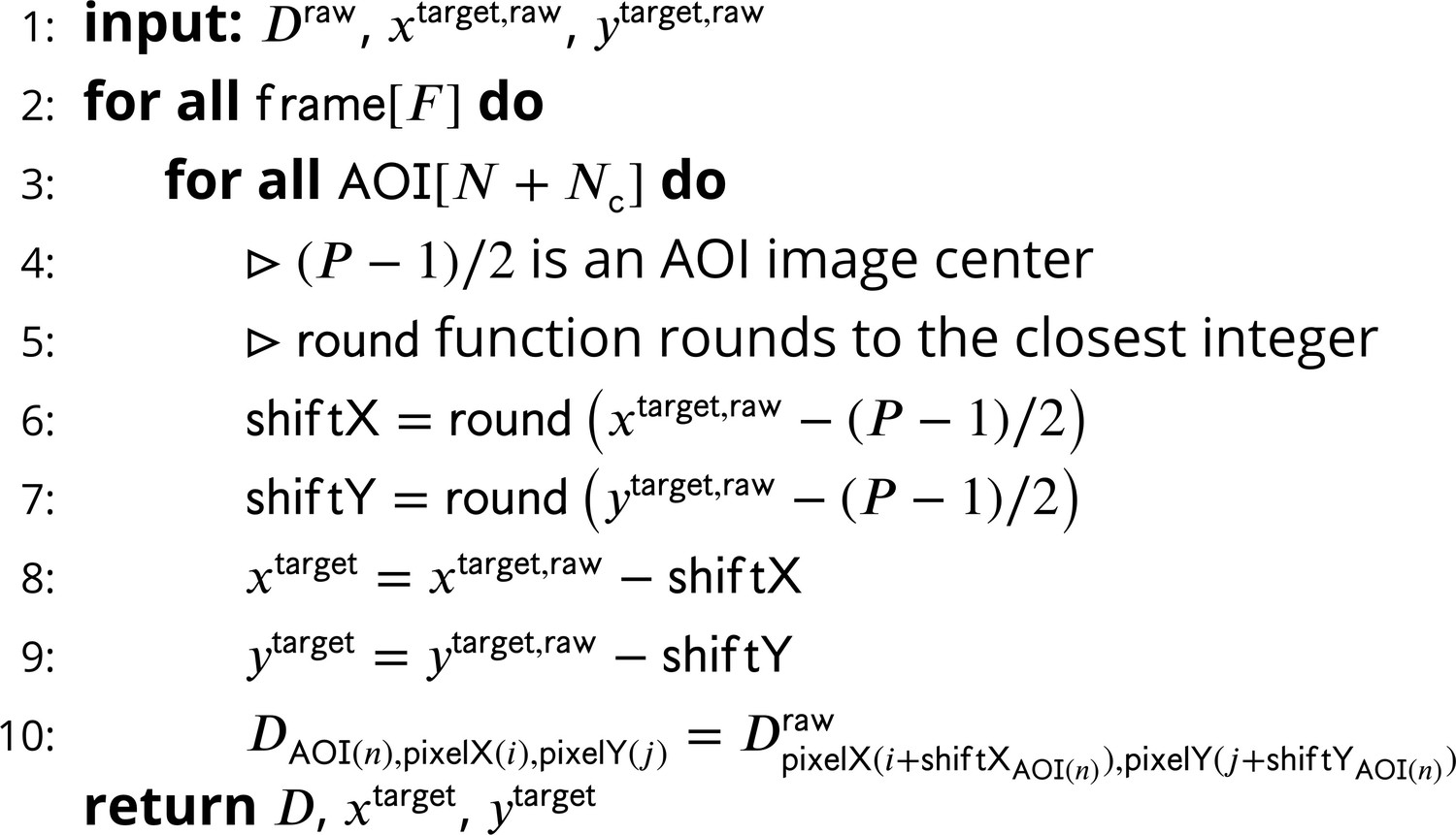
Extraction of AOI images from raw images.

Figure 7—source data 1 Original text for Figure 7.: https://cdn.elifesciences.org/articles/73860/elife-73860-fig7-data1-v2.pdf
Download elife-73860-fig7-data1-v2.pdf

The cosmos model

Our intent is to model CoSMoS image data by accounting for the significant physical aspects of image formation, such as photon noise and binding of target-specific and target-nonspecific molecules to the microscope slide surface. A graphical representation of the Tapqir model for CoSMoS data similar to that in Figure 2D but including probability distributions and other additional detail is shown in Figure 2—figure supplement 1. The corresponding generative model represented as pseudocode is shown in Figure 8. All variables with short descriptions and their domains are listed in Table 3. Below, we describe the model in detail starting with the observed data and the likelihood function and then proceed with model parameters and their prior distributions.

Figure 8

Download asset Open asset

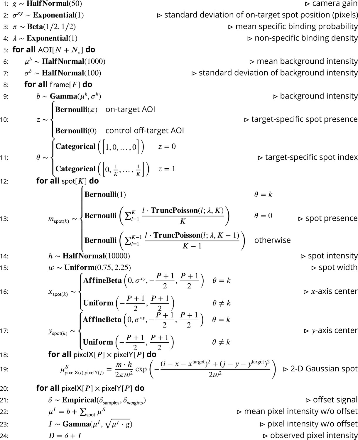
Pseudocode representation of *cosmos* model.

Figure 8—source data 1 Original text for Figure 8.: https://cdn.elifesciences.org/articles/73860/elife-73860-fig8-data1-v2.pdf
Download elife-73860-fig8-data1-v2.pdf

Table 3

Variables used in the Tapqir model.

Symbol	Meaning	Domain
$K$	Maximum number of spots per image	$ℕ$
$N$	Number of on-target AOIs	$ℕ$
$N_{c}$	Number of off-target control AOIs	$ℕ$
$F$	Number of frames	$ℕ$
$P$	Size of the AOI image in pixels	$ℕ$
$g$	Camera gain	$R_{> 0}$
$σ^{x y}$	Proximity	$(0, (P + 1) / \sqrt{12})$
$π$	Average target-specific binding probability	$[0, 1]$
$λ$	Target-nonspecific binding density	$R_{> 0}$
$μ^{b}$	Mean background intensity across AOI	$R_{> 0}^{A O I [N]}$
$σ^{b}$	Standard deviation of background intensity across AOI	$R_{> 0}^{A O I [N]}$
$b$	Background intensity	$R_{> 0}^{A O I [N] \times f r a m e [F]}$
$z$	Target-specific spot presence	${0, 1}^{A O I [N] \times f r a m e [F]}$
$θ$	Target-specific spot index	${0, 1, \dots, K}^{A O I [N] \times f r a m e [F]}$
$m$	Spot presence indicator	${0, 1}^{s p o t [K] \times A O I [N] \times f r a m e [F]}$
$h$	Integrated spot intensity	$R_{> 0}^{s p o t [K] \times A O I [N] \times f r a m e [F]}$
$w$	Spot width	$[0.75, 2.25]^{s p o t [K] \times A O I [N] \times f r a m e [F]}$
$x$	Center of the spot on the $x$ -axis	$R^{s p o t [K] \times A O I [N] \times f r a m e [F]}$
$y$	Center of the spot on the $y$ -axis	$R^{s p o t [K] \times A O I [N] \times f r a m e [F]}$
$μ^{S}$	2-D Gaussian spot	$R_{> 0}^{s p o t [K] \times A O I [N] \times f r a m e [F] \times p i x e l X [P] \times p i x e l Y [P]}$
$μ^{I}$	Ideal image w/o offset	$R_{> 0}^{A O I [N] \times f r a m e [F] \times p i x e l X [P] \times p i x e l Y [P]}$
$δ$	Offset signal	$R_{> 0}^{A O I [N] \times f r a m e [F] \times p i x e l X [P] \times p i x e l Y [P]}$
$I$	Observed image w/o offset signal	$R_{> 0}^{A O I [N] \times f r a m e [F] \times p i x e l X [P] \times p i x e l Y [P]}$
$D$	Observed image ( $I + δ$ )	$R_{> 0}^{A O I [N] \times f r a m e [F] \times p i x e l X [P] \times p i x e l Y [P]}$
$x^{t a r g e t}$	Target molecule position on the $x$ -axis	$[P / 2 - 1, P / 2]^{A O I [N] \times f r a m e [F]}$
$y^{t a r g e t}$	Target molecule position on the $y$ -axis	$[P / 2 - 1, P / 2]^{A O I [N] \times f r a m e [F]}$
i	Pixel index on the $x$ -axis	${0, \dots, (P - 1)}^{p i x e l X [P]}$
$j$	Pixel index on the $y$ -axis	${0, \dots, (P - 1)}^{p i x e l X [P]}$
$W$	Width of the raw microscope images in pixels	$ℕ$
$H$	Height of the raw microscope image in pixels	$ℕ$
$D^{r a w}$	Raw microscope images	$R_{> 0}^{f r a m e [F] \times p i x e l X [H] \times p i x e l Y [W]}$
$x^{t a r g e t, r a w}$	Target molecule position in raw images on the $x$ -axis	$[- 0.5, H - 0.5]^{A O I [N] \times f r a m e [F]}$
$y^{t a r g e t, r a w}$	Target molecule position in raw images on the $y$ -axis	$[- 0.5, W - 0.5]^{A O I [N] \times f r a m e [F]}$

Image likelihood

Request a detailed protocol

We model the image data $D$ as the sum of a photon-independent offset $δ$ introduced by the camera and the noisy photon-dependent pixel intensity values $I$ :

D = δ + I

In our model, each pixel in the photon-dependent image $I$ has a variance which is equal to the mean intensity $μ^{I}$ of that pixel multiplied by the camera gain $g$ , which is the number of camera intensity units per photon. This formulation is appropriate for cameras that use charge-coupled device (CCD) or electron-multiplier CCD (EMCCD) sensors. (The experimental CoSMoS datasets we analyzed (Table 1) were collected with EMCCD cameras.) It accounts for both photon shot noise and additional noise introduced by EMCCD camera amplification (van Vliet et al., 1998) and is expressed using a continuous Gamma distribution:

I \sim G a m m a (μ^{I}, \sqrt{μ^{I} \cdot g})

The Gamma distribution was chosen because we found it to effectively model the image noise, which includes both Poissonian (shot noise) and non-Poissonian contributions. The Gamma distribution used here is parameterized by its mean and standard deviation. The functional forms of the Gamma distribution and all other distributions we use in this work are given in Table 4.

Table 4

Probability distributions used in the model.

Distribution	PDF
$x \sim A f f i n e B e t a (μ, ν, a, b)$	$\frac{y^{α - 1} (1 - y)^{β - 1}}{B (α, β)} w h e r e α = \frac{ν (μ - a)}{b - a}, β = \frac{ν (b - μ)}{b - a}, a n d y = \frac{x - a}{b - a}$
$x \sim B e r n o u l l i (π)$	$π^{x} {(1 - π)}^{1 - x}$
$x \sim B e t a (α, β)$	$\frac{x^{α - 1} {(1 - x)}^{β - 1}}{B (α, β)}$
$x \sim C a t e g o r i c a l (p)$	$\prod_{i = 1}^{k} p_{i}^{[x = i]}$
$x \sim E m p i r i c a l (z, p)$	$\prod_{i = 1}^{k} p_{i}^{[x = z_{i}]}$
$x \sim E x p o n e n t i a l (λ)$	$λ e^{- λ x}$
$x \sim G a m m a (μ, σ)$	$\frac{β^{α}}{Γ (α)} x^{α - 1} e^{- β x} w h e r e α = \frac{μ^{2}}{σ^{2}} a n d β = \frac{μ}{σ^{2}}$
$x \sim H a l f N o r m a l (σ)$	$\frac{\sqrt{2}}{σ \sqrt{π}} \exp (- \frac{x^{2}}{2 σ^{2}}) f o r x > 0$
$k \sim T r u n c P o i s s o n (λ, K)$	${\begin{cases} 1 - e^{- λ} \sum_{i = 0}^{K - 1} \frac{λ^{i}}{i!} & i f k = K \\ \frac{λ^{k} e^{- λ}}{k!} & o t h e r w i s e \end{cases}$
$x \sim U n i f o r m (a, b)$	$\frac{1}{b - a} f o r x \in [a, b]$

A competing camera technology based on scientific complementary metal-oxide semiconductor (sCMOS) sensors produces images that have also successfully been modeled as having a combination of Poissonian and non-Poissonian (Gaussian, in this case) noise sources. However, sCMOS images have noise characteristics that are considerably more complicated than CCD/EMCCD images, because every pixel has its own characteristic intensity offset, Gaussian noise variance, and amplification gain. Additional validation will be required to determine whether the existing cosmos model requires modification or inclusion of additional prior information (e.g., pixel-by-pixel calibration data as in Huang et al., 2013) to optimize its performance with sCMOS CoSMoS data.

Image model

Request a detailed protocol

The idealized noise-free image $μ^{I}$ is represented as the sum of a background intensity $b$ and the intensities from fluorescence spots modeled as 2-D Gaussians $μ^{S}$ :

μ^{I} = b + \sum_{s p o t} μ^{S}

For simplicity, we allow at most $K$ number of spots in each frame of each AOI. (In this article, we always use $K$ equal to 2.) The presence of a given spot in the image is encoded in the binary spot existence parameter $m$ , where $m$ = 1 when the corresponding spot is present and $m$ = 0 when it is absent.

The intensities for a 2-D Gaussian spot at each pixel coordinate (i, $j$ ) is given by:

μ_{p i x e l X (i), p i x e l Y (j)}^{S} = \frac{m \cdot h}{2 π w^{2}} \exp (- \frac{(i - x - x^{t a r g e t})^{2} + (j - y - y^{t a r g e t})^{2}}{2 w^{2}})

with spot parameters total integrated intensity $h$ , width $w$ , and center ( $x$ , $y$ ) relative to the target (or off-target control) location ( $x^{t a r g e t}$ , $y^{t a r g e t}$ ).

Our primary interest is whether a target-specific spot is absent or present in a given AOI. We encode this information using a binary state parameter $z$ with 0 and 1 denoting target-specific spot absence and presence, respectively. To indicate which of the $K$ spots is target-specific, we use the index parameter $θ$ which ranges from 0 to $K$ . When a target-specific spot is present ( $z$ = 1), $θ \in {1, \dots, K}$ specifies the index of the target-specific spot, while $θ$ = 0 indicates that no target-specific spot is present ( $z$ = 0). For example, ${m_{s p o t (1)} = 1, m_{s p o t (2)} = 1, z = 1, θ = 2}$ means that both spots are present and spot 2 is target-specific. A combination like ${m_{s p o t (1)} = 0, m_{s p o t (2)} = 1, z = 1, θ = 1}$ is impossible (i.e., has zero probability) since spot 1 cannot be absent and target-specific at the same time. For off-target control data, in which no spots are target-specific by definition, $z$ and $θ$ are always set to zero.

Prior distributions

Request a detailed protocol

The prior distributions for the model parameters are summarized in Figure 2—figure supplement 1 and detailed below. Unless otherwise indicated we assume largely uninformative priors (such as the Half-Normal distribution with large mean).

Background intensity $b$ follows a Gamma distribution:

b \sim G a m m a (μ^{b}, σ^{b})

where the mean $μ^{b} \in R_{> 0}^{A O I [N]}$ and standard deviation $σ^{b} \in R_{> 0}^{A O I [N]}$ of the background intensity describe the irregularity in the background intensity in time and across the field of view of the microscope. Priors for $μ^{b}$ and $σ^{b}$ are uninformative:

μ^{b} \sim H a l f N o r m a l (1000)

σ^{b} \sim H a l f N o r m a l (100)

The target-specific presence parameter $z$ has a Bernoulli prior parameterized by the average target-specific binding probability $π$ for on-target AOIs and zero probability for control off-target AOIs:

z \sim {\begin{cases} B e r n o u l l i (π) & on-target AOI \\ 0 & control off-target AOI \end{cases}

The prior distribution for the index of the target-specific spot $θ$ is conditional on $z$ . When no specifically bound spot is present (i.e., $z$ = 0), $θ$ always equals 0. Since spot indices are arbitrarily assigned, when the target-specific spot is present (i.e., $z$ = 1) $θ$ can take any value between 1 and $K$ with equal probability. We represent the prior for $θ$ as a Categorical distribution of the following form:

θ \sim {\begin{cases} 0 & z = 0 \\ C a t e g o r i c a l ([\begin{matrix} 0, \frac{1}{K}, \dots, \frac{1}{K} \end{matrix}]) & z = 1 \end{cases}

The average target-specific binding probability $π$ has an uninformative Jeffreys prior (Gelman et al., 2013) given by a Beta distribution:

π \sim B e t a (1 / 2, 1 / 2)

The prior distribution for the spot presence indicator $m$ is conditional on $θ$ . When $θ$ corresponds to spot index $k$ , i.e., $θ = k$ , then $m_{s p o t (k)}$ = 1. When $θ$ does not correspond to a spot index $k$ , that is, $θ \neq k$ , then either spot $k$ is target-nonspecific or a spot corresponding to $k$ does not exist. Consequently, for $θ \neq k$ we assign $m_{s p o t (k)}$ to either 0 or 1 with a probability dependent on the non-specific binding density $λ \in R_{> 0}$ :

m_{s p o t} (k) \sim {\begin{cases} 1 & θ = k \\ B e r n o u l l i (\sum_{l = 1}^{K} \frac{l \cdot T r u n c P o i s s o n (l; λ, K)}{K}) & θ = 0 \\ B e r n o u l l i (\sum_{l = 1}^{K - 1} \frac{l \cdot T r u n c P o i s s o n (l; λ, K - 1)}{K - 1}) & otherwise \end{cases}

The mean non-specific binding density $λ$ is expected to be much less than two non-specifically bound spots per frame per AOI; therefore, we use an Exponential prior of the form

λ \sim E x p o n e n t i a l (1)

The prior distribution for the integrated spot intensity $h$ is chosen to fall off at a value much greater than typical spot intensity values

h \sim H a l f N o r m a l (10000)

In CoSMoS experiments, the microscope/camera hardware is typically designed to set the width $w$ of fluorescence spots to a typical value in the range of 1–2 pixels (Ober et al., 2015). We use a Uniform prior confined to the range between 0.75 and 2.25 pixels:

w \sim U n i f o r m (0.75, 2.25)

Priors for spot position ( $x$ , $y$ ) depend on whether the spot represents target-specific or non-specific binding. Non-specific binding to the microscope slide surface can occur anywhere within the image and therefore has a uniform distribution (Figure 2—figure supplement 2, red). Spot centers may fall slightly outside the AOI image yet still affect pixel intensities within the AOI. Therefore the range for ( $x$ , $y$ ) is extended one pixel wider than the size of the image, which allows a spot center to fall slightly beyond the AOI boundary.

In contrast to non-specifically bound molecules, specifically bound molecules are colocalized with the target molecule with a precision that can be better than one pixel and that depends on various factors including the microscope point-spread function and magnification, accuracy of registration between binder and target image channels, and accuracy of drift correction. For target-specific binding, we use an Affine-Beta prior with zero mean position relative to the target molecule location ( $x^{t a r g e t}$ , $y^{t a r g e t}$ ), and a ‘proximity’ parameter $σ^{x y}$ which is the standard deviation of the Affine-Beta distribution (Figure 2—figure supplement 2, green). We chose the Affine-Beta distribution because it models a continuous parameter defined on a bounded interval.

x_{s p o t (k)}, y_{s p o t (k)} \sim {\begin{cases} A f f i n e B e t a (0, σ^{x y}, - \frac{P + 1}{2}, \frac{P + 1}{2}) & θ = k (target-specific) \\ U n i f o r m (- \frac{P + 1}{2}, \frac{P + 1}{2}) & θ \neq k (target-nonspecific) \end{cases}

We give the proximity parameter $σ^{x y}$ a diffuse prior, an Exponential with a characteristic width of one pixel:

σ^{x y} \sim E x p o n e n t i a l (1)

Tests on data simulated with increasing proximity parameter values $σ^{x y}$ (true) (i.e., with decreasing precision of spatial mapping between the binder and target image channels) confirm that the cosmos model accurately learns $σ^{x y}$ (fit) from the data (Figure 3—figure supplement 3D; Table 5). This was the case even if we substituted a less-informative $σ^{x y}$ prior (Uniform vs. Exponential; Table 5).

Table 5

The effect of mapping precision on classification accuracy*.

$σ^{x y}$ (true)	$σ^{x y}$ (fit) [95% CI]	MCC	$σ^{x y}$ Prior
0.2	0.21 [0.20, 0.22]	0.989	$E x p o n e n t i a l (1)$
1	0.96 [0.90, 1.02]	0.939	$E x p o n e n t i a l (1)$
1.5	1.49 [1.40, 1.59]	0.890	$E x p o n e n t i a l (1)$
2	1.96 [1.84, 2.09]	0.834	$E x p o n e n t i a l (1)$
2	1.97 [1.84, 2.09]	0.834	$U n i f o r m (0, (P + 1) / \sqrt{12})$

*

Data were simulated over a range of proximity parameter $σ^{x y}$ values at fixed $π = 0.15$ and $λ = 0.15$ (Supplementary file 6).

The CoSMoS technique is premised on colocalization of the binder spots with the known location of the target molecule. Consequently, for any analysis method, classification accuracy declines when the images in the target and binder channels are less accurately mapped. For the Tapqir cosmos model, low mapping precision has little effect on classification accuracy at typical non-specific binding densities ( $λ$ = 0.15; see MCC values in Table 5).

Gain $g$ depends on the settings of the amplifier and electron multiplier (if present) in the camera. It has a positive value and is typically in the range between 5 and 50. We use a Half-Normal prior with a broad distribution encompassing this range:

g \sim H a l f N o r m a l (50)

The prior distribution for the offset signal $δ$ is empirically measured from the output of camera sensor regions that are masked from incoming photons. Collected data from these pixels are transformed into a density histogram with intensity step size of 1. The resulting histogram typically has a long right hand tail of low density. For computational efficiency, we shorten this tail by binning together pixel intensity values from the upper 0.5% percentile. Since $D = δ + I$ (Equation 1) and photon-dependent intensity $I$ is positive, all $D$ values have to be larger than the smallest offset intensity value. If that is not the case we add a single value $\min (D) - 1$ to the offset empirical distribution which has a negligible effect on the distribution. Bin values $δ_{s a m p l e s}$ and their weights $δ_{w e i g h t s}$ are used to construct an Empirical prior:

δ \sim E m p i r i c a l (δ_{s a m p l e s}, δ_{w e i g h t s})

All simulated and experimental data sets in this work were analyzed using the prior distributions and hyperparameter values given above, which are compatible with a broad range of experimental conditions (Table 1). Many of the priors are uninformative and we anticipate that these will work well with images taken on variety of microscope hardware. However, it is possible that highly atypical microscope designs (e.g., those with effective magnifications that are sub-optimal for CoSMoS) might require adjustment of some fixed hyperparameters and distributions (those in Eqs. 6a, 6b, 11, 12, 13, 15, and 16). For example, if the microscope point spread function is more than 2 pixels wide, it may be necessary to increase the range of the $w$ prior in Eq. 13. The Tapqir documentation (https://tapqir.readthedocs.io/en/stable/) gives instructions for changing the hyperparameters.

Joint distribution

Request a detailed protocol

The joint distribution of the data and all parameters is the fundamental distribution necessary to perform a Bayesian analysis. Let $ϕ$ be the set of all model parameters. The joint distribution can be expressed in a factorized form:

\begin{aligned} p (D, ϕ) = & p (g) p (σ^{x y}) p (π) p (λ) \prod_{A O I} [p (μ^{b}) p (σ^{b}) \prod_{f r a m e} [p (b | μ^{b}, σ^{b}) p (z | π) p (θ | z) \cdot \\ \prod_{s p o t} [p (m | θ, λ) p (h) p (w) p (x | σ^{x y}, θ) p (y | σ^{x y}, θ)] \prod_{\begin{matrix} p i x e l X \\ p i x e l Y \end{matrix}} p (δ) p (D | μ^{I}, g, δ)]] \end{aligned}

The Tapqir generative model is a stochastic function that describes a properly normalized joint distribution for the data and all parameters (Figure 8). In Pyro this is called ‘the model’.

Inference

Request a detailed protocol

For a Bayesian analysis, we want to obtain the posterior distribution for parameters $ϕ$ given the observed data $D$ . There are three discrete parameters $z$ , $θ$ , and $δ$ that can be marginalized out exactly so that they do not appear expilictly in either the joint posterior distribution or the likelihood function. Computationally efficient marginalization is implemented using Pyro’s enumeration strategy (Obermeyer et al., 2019a) and KeOps’ kernel operations on the GPU without memory overflows (Charlier et al., 2021). Let $ϕ^{'} = ϕ - {z, θ, δ}$ be the rest of the parameters. We obtain posterior distributions of $ϕ^{'}$ using Bayes’ rule:

p (ϕ^{'} | D) = \frac{\sum_{z, θ, δ} p (D, ϕ)}{\int_{ϕ} p (D, ϕ) d ϕ} = \frac{p (D, ϕ^{'})}{\int_{ϕ} p (D, ϕ) d ϕ} = \frac{p (D | ϕ^{'}) p (ϕ^{'})}{\int_{ϕ} p (D, ϕ) d ϕ}

Note that the integral in the denominator of this expression is necessary to calculate the posterior distribution, but it is usually analytically intractable. However, variational inference provides a robust method to approximate the posterior distribution $p (ϕ^{'} ∣ D)$ with a parameterized variational distribution $q (ϕ^{'})$ (Bishop, 2006).

p (ϕ^{'} | D) ≃ q (ϕ^{'})

$q (ϕ^{'})$ has the following factorization:

\begin{aligned} q (ϕ^{'}) = & q (g) q (σ^{x y}) q (π) q (λ) \cdot \\ \prod_{A O I} [q (μ^{b}) q (σ^{b}) \prod_{f r a m e} [q (b) \prod_{s p o t} [q (m) q (h | m) q (w | m) q (x | m) q (y | m)]]] \end{aligned}

The variational distribution $q (ϕ^{'})$ is provided as pseudocode for a generative stochastic function (Figure 9). In Pyro this is called ‘the guide’. Variational inference is sensitive to initial values of variational parameters. In Figure 9, step 1 we provide the initial values of variational parameters used in our analyses.

Figure 9

Download asset Open asset

Pseudocode representation of *cosmos* guide.

Figure 9—source data 1 Original text for Figure 9.: https://cdn.elifesciences.org/articles/73860/elife-73860-fig9-data1-v2.pdf
Download elife-73860-fig9-data1-v2.pdf

Calculation of spot probabilities

Request a detailed protocol

Variational inference directly optimizes $q (m) \equiv m_{p r o b}$ (see Eq. 21 and Figure 9), which approximates $p (m | D)$ . To obtain the marginal posterior probabilities $p (z, θ | D)$ , we use a Monte Carlo sampling method:

\begin{array}{ll} p (z, θ | D) & = \int_{ϕ^{'}} p (z, θ, ϕ^{'} | D) d ϕ^{'} \\ = \int_{ϕ^{'}} p (z, θ | ϕ^{'}, D) p (ϕ^{'} | D) d ϕ^{'} \\ = \int_{ϕ^{'}} p (z, θ | ϕ^{'}, D) p (ϕ^{'} | D) d ϕ^{'} \\ = \int_{ϕ^{'}} \frac{p (z, θ, ϕ^{'}, D)}{\sum_{z, θ} p (z, θ, ϕ^{'}, D)} p (ϕ^{'} | D) d ϕ^{'} \\ ≃ \frac{1}{S} \sum_{s = 1}^{S} \frac{p (z, θ, ϕ_{s}^{'}, D)}{\sum_{z, θ} p (z, θ, ϕ_{s}^{'}, D)} where ϕ_{s}^{'} \sim q (ϕ^{'}) \end{array}

In our calculations, we used $S$ = 25 as the number of Monte Carlo samples. Marginal probabilities $p (z | D)$ and $p (θ | D)$ are calculated as:

p (z | D) = \sum_{θ} p (z, θ | D)

p (θ | D) = \sum_{z} p (z, θ | D)

The probability, $p (s p e c i f i c)$ , that a target-specific fluorescence spot is present in a given image by definition is:

p (s p e c i f i c) \equiv p (z = 1 | D)

For simplicity in the main text and figures we suppress the conditional dependency on $D$ in $p (θ | D)$ and $p (m | D)$ and instead write them as $p (θ)$ and $p (m)$ , respectively.

Tapqir implementation

Request a detailed protocol

The model and variational inference method outlined above are implemented as a probabilistic program in the Python-based probabilistic programming language (PPL) Pyro (Foerster et al., 2018; Bingham et al., 2019; Obermeyer et al., 2019a). We use a variational approximation because exact inference is not analytically tractable for a model as complex as cosmos. As currently implemented in Pyro, variational inference is significantly faster than Monte Carlo inference methods. In Tapqir, the objective that is being optimized is the evidence lower bound (ELBO) estimator that provides unbiased gradient estimates upon differentiation. At each iteration of inference procedure we choose a random subset of AOIs and frames (mini-batch), compute a differentiable ELBO estimate based on this mini-batch and update the variational parameters via automatic differentiation. We use PyTorch’s Adam optimizer (Kingma and Ba, 2014) with the learning rate of $5 \times 10^{- 3}$ and keep other parameters at their default values.

Credible intervals and confidence intervals

Request a detailed protocol

Credible intervals were calculated from posterior distribution samples as the highest density region (HDR), the narrowest interval with probability mass 95% using the pyro.ops.stats.hpdi Pyro function. Confidence intervals were calculated from bootstrap samples as the 95% HDR.

Data simulation

Request a detailed protocol

Simulated data were produced using the generative model (Figure 8). Each simulation has a subset of parameters ( $π, λ$ , $g$ , $σ^{x y}$ , $b$ , $h$ , $w, δ$ ) set to desired values while the remaining parameters ( $z, θ$ , $m$ , $x$ , $y$ ) and resulting noisy images ( $D$ ) are sampled from distributions. The fixed parameter values and data set sizes for all simulations are provided inSupplementary file 1; Supplementary file 2; Supplementary file 3; Supplementary file 4; Supplementary file 5; Supplementary file 6.

For kinetic simulations (Figure 5, Supplementary file 5), $z$ was modeled using a discrete Markov process with the initial probability and the transition probability matrices:

p (z_{f r a m e (0)} | k_{o n}, k_{o f f}) = C a t e g o r i c a l ([\begin{matrix} \frac{k_{o f f}}{k_{o n} + k_{o f f}} & \frac{k_{o n}}{k_{o n} + k_{o f f}} \end{matrix}])

p (z_{f r a m e (f)} | z_{f r a m e (f - 1)}, k_{o n}, k_{o f f}) = C a t e g o r i c a l ([\begin{matrix} 1 - k_{o n} & k_{o n} \\ k_{o f f} & 1 - k_{o f f} \end{matrix}])

where $k_{o n}$ and $k_{o f f}$ are transition probabilities that numerically approximate the pseudo-first-order binding and first-order dissociation rate constants in units of $s^{- 1}$ , respectively, assuming 1 s/frame. We assumed that the Markov process is at equilibrium and initialized the chain with the equilibrium probabilities.

Posterior predictive sampling

Request a detailed protocol

For posterior predictive checking, sampled images ( $\tilde{D}$ ) were produced using Tapqir’s generative model (Figure 8) where model parameters were sampled from the posterior distribution $p (ϕ | D)$ , which was approximated by the variational distribution $q (ϕ)$ :

\begin{aligned} \tilde{D} \sim p (\tilde{D} | D) & = \int_{ϕ} p (\tilde{D} | ϕ) p (ϕ | D) d ϕ \\ ≃ \int_{ϕ} p (\tilde{D} | ϕ) q (ϕ) d ϕ \end{aligned}

Signal-to-noise ratio

Request a detailed protocol

We define SNR as:

S N R = m e a n (\frac{s i g n a l}{\sqrt{σ_{o f f s e t}^{2} + σ_{b a c k g r o u n d}^{2}}})

where $σ_{b a c k g r o u n d}^{2} = b \cdot g$ the variance of the background intensity, $σ_{o f f s e t}^{2}$ the variance of the offset intensity, and the mean is taken over all target-specific spots. For experimental data, $s i g n a l$ is calculated as

s i g n a l = \sum_{\begin{matrix} p i x e l X \\ p i x e l Y \end{matrix}} (D - b_{m e a n} - δ_{m e a n}) \cdot w e i g h t

where $w e i g h t$ is

w e i g h t = \frac{1}{2 π \cdot w^{2}} \exp (- \frac{(i - x - x^{t a r g e t})^{2} + (j - y - y^{t a r g e t})^{2}}{2 \cdot w^{2}})

For simulated data theoretical $s i g n a l$ is directly calculated as:

s i g n a l = \sum_{\begin{matrix} p i x e l X \\ p i x e l Y \end{matrix}} h \cdot {w e i g h t}^{2}

Classification accuracy statistics

Request a detailed protocol

As a metric of classification accuracy we use three commonly used statistics – recall, precision, and Matthews Correlation Coefficient (Matthews, 1975)

R e c a l l = \frac{T P}{T P + F N}

P r e c i s i o n = \frac{T P}{T P + F P}

M C C = \frac{T P \cdot T N - F P \cdot F N}{\sqrt{(T P + F P) (T P + F N) (T N + F P) (T N + F N)}}

where TP is true positives, TN is true negatives, FP is false positives, and FN is false negatives.

Kinetic and thermodynamic analysis

Request a detailed protocol

To estimate simple binding/dissociation kinetic parameters (Figure 5C and D), we sample binary time records $z$ from the inferred $p (s p e c i f i c)$ time records for all AOIs. For a two-state hidden Markov model, the maximum-likelihood estimates of $k_{o n}$ and $k_{o f f}$ are given by:

{\hat{k}}_{o n}, {\hat{k}}_{o f f} = \underset{k_{o n}, k_{o f f}}{argmax} \prod_{A O I} [p (z_{f r a m e (0)} | k_{o n}, k_{o f f}) \prod_{f = 1}^{F - 1} p (z_{f r a m e (f)} | z_{f r a m e (f - 1)}, k_{o n}, k_{o f f})]

Repeating this procedure 2,000 times gave the distributions of $k_{o n}$ and $k_{o f f}$ from which we compute mean and 95% credible interval.

Similarly, to estimate mean and 95% CI of $K_{e q}$ (Figure 5E) we sampled π from $q (π)$ and for each sampled value of $π$ calculated $K_{e q}$ as:

K_{e q} = \frac{π}{1 - π}

To calculate time-to-first binding kinetics from the Tapqir-derived $p (s p e c i f i c)$ (Figure 6B, Figure 6—figure supplement 1B, Figure 6—figure supplement 2B, and Figure 6—figure supplement 3B), 2,000 binary time records $z$ were sampled from the $p (s p e c i f i c)$ time record for each AOI. For each sampled time record initial absent intervals were measured and analyzed using Equation 7 in Friedman and Gelles, 2015, yielding distributions of $k_{a}$ , $k_{n s}$ , and $A_{f}$ . Mean value and 95% credible intervals were calculated from these distributions. Initial absent intervals from ‘spot-picker’ analysis (Figure 6C, Figure 6—figure supplement 1C, Figure 6—figure supplement 2C, and Figure 6—figure supplement 3C) were analyzed as described in Friedman and Gelles, 2015, except that on-target and off-target data were here analyzed jointly instead of being analyzed sequentially (Friedman and Gelles, 2015). Note that the $k_{n s}$ values determined using the two methods are not directly comparable for several reasons, including that the non-specific binding frequencies are effectively measured over different areas. For Tapqir, the target area is approximately $π {(σ^{x y})}^{2}$ (which is between 0.3 and 0.8 pixels² in the different experimental data sets) and for spot-picker the area is subjectively chosen as $π \cdot {1.5}^{2} = 7$ pixels².

Data availability

All data generated or analyzed for this study will be available at https://github.com/ordabayevy/tapqir-overleaf. That repository also includes all figures, figure supplements, and the scripts and data used to generate them. It also contains the supplemental data files and preprint manuscript text.

The following data sets were generated

(2022) Github
ID ordabayevy/tapqir-overleaf. Simulated and experimental data used for "Bayesian machine learning analysis of single-molecule fluorescence colocalization images".

https://github.com/ordabayevy/tapqir-overleaf

References

1. Bingham E
2. Chen JP
3. Jankowiak M
4. Obermeyer F
5. Pradhan N
6. Karaletsos T
7. Singh R
8. Szerlip P
9. Horsfall P
10. Goodman ND
(2019)
Pyro: Deep universal probabilistic programming

Journal of Machine Learning Research: JMLR 20:1–6.
- Google Scholar
Book
1. Bishop CM
(2006)
Pattern Recognition and Machine Learning

New York: Springer.
- Google Scholar
(2012) Rocket launcher mechanism of collaborative actin assembly defined by single-molecule imaging
Science (New York, N.Y.) 336:1164–1168.
https://doi.org/10.1126/science.1218062
- PubMed
- Google Scholar
1. Charlier B
2. Feydy J
3. Glaunès JA
4. Collin FD
5. Durif G
(2021)
Kernel operations on the GPU, with autodiff, without memory overflows

Journal of Machine Learning Research: JMLR 22:1–6.
- Google Scholar
1. Chen J
2. Dalal RV
3. Petrov AN
4. Tsai A
5. O’Leary SE
6. Chapin K
7. Cheng J
8. Ewan M
9. Hsiung PL
10. Lundquist P
11. Turner SW
12. Hsu DR
13. Puglisi JD
(2014) High-throughput platform for real-time monitoring of biological processes by multicolor single-molecule fluorescence
PNAS 111:664–669.
https://doi.org/10.1073/pnas.1315735111
- PubMed
- Google Scholar
Preprint
1. Chiang D
2. Rush AM
3. Barak B
(2021) Named Tensor Notation
arXiv.

https://arxiv.org/abs/2102.13196
- Google Scholar
1. Fawcett T
(2006) An introduction to ROC analysis
Pattern Recognition Letters 27:861–874.
https://doi.org/10.1016/j.patrec.2005.10.010
- Google Scholar
Preprint
(2018) DiCE: The Infinitely Differentiable Monte-Carlo Estimator
arXiv.

https://arxiv.org/abs/1802.05098
- Google Scholar
(2006) Viewing dynamic assembly of molecular complexes by multi-wavelength single-molecule fluorescence
Biophysical Journal 91:1023–1031.
https://doi.org/10.1529/biophysj.106.084004
- PubMed
- Google Scholar
1. Friedman LJ
2. Gelles J
(2012) Mechanism of transcription initiation at an activator-dependent promoter defined by single-molecule observation
Cell 148:679–689.
https://doi.org/10.1016/j.cell.2012.01.018
- PubMed
- Google Scholar
(2013) RNA polymerase approaches its promoter without long-range sliding along DNA
PNAS 110:9740–9745.
https://doi.org/10.1073/pnas.1300221110
- PubMed
- Google Scholar
1. Friedman LJ
2. Gelles J
(2015) Multi-wavelength single-molecule fluorescence analysis of transcription mechanisms
Methods (San Diego, Calif.) 86:27–36.
https://doi.org/10.1016/j.ymeth.2015.05.026
- PubMed
- Google Scholar
(2014) Single-molecule studies of polymerase dynamics and stoichiometry at the bacteriophage T7 replication machinery
PNAS 111:4073–4078.
https://doi.org/10.1073/pnas.1402010111
- PubMed
- Google Scholar
Book
1. Gelman A
2. Carlin JB
3. Stern HS
4. Dunson DB
5. Vehtari A
6. Rubin DB
(2013) Chapman and Hall/CRC Texts in Statistical Science
Philadelphia: CRC Press.
https://doi.org/10.1201/b16018
- Google Scholar
1. Huang F
2. Hartwich TMP
3. Rivera-Molina FE
4. Lin Y
5. Duim WC
6. Long JJ
7. Uchil PD
8. Myers JR
9. Baird MA
10. Mothes W
11. Davidson MW
12. Toomre D
13. Bewersdorf J
(2013) Video-rate nanoscopy using sCMOS camera-specific single-molecule localization algorithms
Nature Methods 10:653–658.
https://doi.org/10.1038/nmeth.2488
- PubMed
- Google Scholar
(2014) Protein-guided RNA dynamics during early ribosome assembly
Nature 506:334–338.
https://doi.org/10.1038/nature13039
- PubMed
- Google Scholar
Preprint
1. Kingma DP
2. Ba J
(2014) Adam: A Method for Stochastic Optimization
arXiv.

https://arxiv.org/abs/1412.6980
- Google Scholar
(2021) Bayesian Inference: The Comprehensive Approach to Analyzing Single-Molecule Experiments
Annual Review of Biophysics 50:191–208.
https://doi.org/10.1146/annurev-biophys-082120-103921
- PubMed
- Google Scholar
(2013) Biased Brownian ratcheting leads to pre-mRNA remodeling and capture prior to first-step splicing
Nature Structural & Molecular Biology 20:1450–1457.
https://doi.org/10.1038/nsmb.2704
- PubMed
- Google Scholar
1. Larson J
2. Kirk M
3. Drier EA
4. O’Brien W
5. MacKay JF
6. Friedman LJ
7. Hoskins AA
(2014) Design and construction of a multiwavelength, micromirror total internal reflectance fluorescence microscope
Nature Protocols 9:2317–2328.
https://doi.org/10.1038/nprot.2014.155
- PubMed
- Google Scholar
1. Lu Y
2. Lee B
3. King RW
4. Finley D
5. Kirschner MW
(2015a) Substrate degradation by the proteasome: a single-molecule kinetic analysis
Science (New York, N.Y.) 348:1250834.
https://doi.org/10.1126/science.1250834
- PubMed
- Google Scholar
1. Lu Y
2. Wang W
3. Kirschner MW
(2015b) Specificity of the anaphase-promoting complex: a single-molecule study
Science (New York, N.Y.) 348:1248737.
https://doi.org/10.1126/science.1248737
- PubMed
- Google Scholar
1. Matthews BW
(1975) Comparison of the predicted and observed secondary structure of T4 phage lysozyme
Biochimica et Biophysica Acta 405:442–451.
https://doi.org/10.1016/0005-2795(75)90109-9
- PubMed
- Google Scholar
1. Noriega TR
2. Chen J
3. Walter P
4. Puglisi JD
(2014) Real-time observation of signal recognition particle binding to actively translating ribosomes
eLife 3:e04418.
https://doi.org/10.7554/eLife.04418
- PubMed
- Google Scholar
1. Ober RJ
2. Tahmasbi A
3. Ram S
4. Lin Z
5. Ward ES
(2015) Quantitative Aspects of Single Molecule Microscopy
IEEE Signal Processing Magazine 32:58–69.
https://doi.org/10.1109/MSP.2014.2353664
- PubMed
- Google Scholar
Preprint
1. Obermeyer F
2. Bingham E
3. Jankowiak M
4. Chiu J
5. Pradhan N
6. Rush A
7. Goodman N
(2019a) Tensor Variable Elimination for Plated Factor Graphs
arXiv.

https://arxiv.org/abs/1902.03210
- Google Scholar
Preprint
1. Obermeyer F
2. Bingham E
3. Jankowiak M
4. Phan D
5. Chen JP
(2019b) Functional Tensors for Probabilistic Programming
arXiv.

https://arxiv.org/abs/1910.10775
- Google Scholar
(2013) Dynamic recognition of the mRNA cap by Saccharomyces cerevisiae eIF4E
Structure (London, England 21:2197–2207.
https://doi.org/10.1016/j.str.2013.09.016
- PubMed
- Google Scholar
1. Peng S
2. Wang W
3. Chen C
(2018) Breaking the Concentration Barrier for Single-Molecule Fluorescence Measurements
Chemistry (Weinheim an Der Bergstrasse, Germany) 24:1002–1009.
https://doi.org/10.1002/chem.201704065
- PubMed
- Google Scholar
1. Rosen GA
2. Baek I
3. Friedman LJ
4. Joo YJ
5. Buratowski S
6. Gelles J
(2020) Dynamics of RNA polymerase II and elongation factor Spt4/5 recruitment during activator-dependent transcription
PNAS 117:32348–32357.
https://doi.org/10.1073/pnas.2011224117
- PubMed
- Google Scholar
1. Roy R
2. Hohng S
3. Ha T
(2008) A practical guide to single-molecule FRET
Nature Methods 5:507–516.
https://doi.org/10.1038/nmeth.1208
- PubMed
- Google Scholar
1. Salomon WE
2. Jolly SM
3. Moore MJ
4. Zamore PD
5. Serebrov V
(2015) Single-Molecule Imaging Reveals that Argonaute Reshapes the Binding Properties of Its Nucleic Acid Guides
Cell 162:84–95.
https://doi.org/10.1016/j.cell.2015.06.029
- PubMed
- Google Scholar
Preprint
1. Särkkä S
2. García-Fernández ÁF
(2019) Temporal Parallelization of Bayesian Smoothers
arXiv.

https://arxiv.org/abs/1905.13002
- Google Scholar
(2013) Alternative spliceosome assembly pathways revealed by single-molecule fluorescence microscopy
Cell Reports 5:151–165.
https://doi.org/10.1016/j.celrep.2013.08.026
- PubMed
- Google Scholar
(2013) Three-color single molecule imaging shows WASP detachment from Arp2/3 complex triggers actin filament branch formation
eLife 2:e01008.
https://doi.org/10.7554/eLife.01008
- PubMed
- Google Scholar
1. Smith CS
2. Stallinga S
3. Lidke KA
4. Rieger B
5. Grunwald D
(2015) Probability-based particle detection that enables threshold-free and robust in vivo single-molecule tracking
Molecular Biology of the Cell 26:4057–4062.
https://doi.org/10.1091/mbc.E15-06-0448
- PubMed
- Google Scholar
1. Smith CS
2. Jouravleva K
3. Huisman M
4. Jolly SM
5. Zamore PD
6. Grunwald D
(2019) An automated Bayesian pipeline for rapid analysis of single-molecule binding data
Nature Communications 10:272.
https://doi.org/10.1038/s41467-018-08045-5
- PubMed
- Google Scholar
1. Tetone LE
2. Friedman LJ
3. Osborne ML
4. Ravi H
5. Kyzer S
6. Stumper SK
7. Mooney RA
8. Landick R
9. Gelles J
(2017) Dynamics of GreB-RNA polymerase interaction allow a proofreading accessory protein to patrol for transcription complexes needing rescue
PNAS 114:E1081–E1090.
https://doi.org/10.1073/pnas.1616525114
- PubMed
- Google Scholar
1. Ticau S
2. Friedman LJ
3. Ivica NA
4. Gelles J
5. Bell SP
(2015) Single-molecule studies of origin licensing reveal mechanisms ensuring bidirectional helicase loading
Cell 161:513–525.
https://doi.org/10.1016/j.cell.2015.03.012
- PubMed
- Google Scholar
1. Tsai A
2. Kornberg G
3. Johansson M
4. Chen J
5. Puglisi JD
(2014) The dynamics of SecM-induced translational stalling
Cell Reports 7:1521–1533.
https://doi.org/10.1016/j.celrep.2014.04.033
- PubMed
- Google Scholar
Preprint
1. van de Meent JW
2. Paige B
3. Yang H
4. Wood F
(2018) An Introduction to Probabilistic Programming
arXiv.

https://arxiv.org/abs/1809.10756
- Google Scholar
1. van Oijen AM
(2011) Single-molecule approaches to characterizing kinetics of biomolecular interactions
Current Opinion in Biotechnology 22:75–80.
https://doi.org/10.1016/j.copbio.2010.10.002
- PubMed
- Google Scholar
Book
(1998)
Digital fluorescence imaging using cooled CCD array cameras invisible

In: Celis JE, editors. Cell Biology. New York: Academic Press. pp. 109–120.
- Google Scholar
(2015) Ribosomal initiation complex-driven changes in the stability and dynamics of initiation factor 2 regulate the fidelity of translation initiation
Journal of Molecular Biology 427:1819–1834.
https://doi.org/10.1016/j.jmb.2014.12.025
- PubMed
- Google Scholar
1. Warnasooriya C
2. Rueda D
(2014) Single-molecule fluorescence-based studies on the dynamics, assembly and catalytic mechanism of the spliceosome
Biochemical Society Transactions 42:1211–1218.
https://doi.org/10.1042/BST20140105
- PubMed
- Google Scholar
(2007) Gaussian approximations of fluorescence microscope point-spread function models
Applied Optics 46:1819–1829.
https://doi.org/10.1364/ao.46.001819
- PubMed
- Google Scholar
1. Zhang Y
2. Feng Y
3. Chatterjee S
4. Tuske S
5. Ho MX
6. Arnold E
7. Ebright RH
(2012) Structural basis of transcription initiation
Science (New York, N.Y.) 338:1076–1080.
https://doi.org/10.1126/science.1227786
- PubMed
- Google Scholar

Decision letter

Ruben L Gonzalez

Reviewing Editor; Columbia University, United States
José D Faraldo-Gómez

Senior Editor; National Heart, Lung and Blood Institute, National Institutes of Health, United States
Colin Kinz-Thompson

Reviewer; Rutgers, United States

Our editorial process produces two outputs: i) public reviews designed to be posted alongside the preprint for the benefit of readers; ii) feedback on the manuscript for the authors, including requests for revisions, shown below. We also include an acceptance summary that explains what the editors found interesting or important about the work.

Decision letter after peer review:

Thank you for submitting your article "Bayesian machine learning analysis of single-molecule fluorescence colocalization images" for consideration by eLife. Your article has been reviewed by 3 peer reviewers, one of whom is a member of our Board of Reviewing Editors, and the evaluation has been overseen by José Faraldo-Gómez as the Senior Editor. The following individual involved in review of your submission has agreed to reveal their identity: Colin Kinz-Thompson (Reviewer #2).

The reviewers have discussed their reviews with one another, and the Reviewing Editor has drafted this to help you prepare a revised submission.

Essential revisions:

1) The γ-distributed noise model used in Tapqir captures quite a lot of physics and, given the analyses in Figures 3-6, clearly works, but might be limited to certain types of cameras used in the fluorescence microscopy (e.g., EMCCDs). For instance, sCMOS cameras have pixel-dependent amplification and noise profiles, rather than a single gain parameter, and are sometimes approximately modeled as normal distributions with both mean and variance having intensity-dependent and intensity-independent contributions that are different for each pixel on the camera. The authors should therefore address the question of whether Tapqir can also be used with data collected from different cameras and, specifically, sCMOS cameras.

2) Little information is included about the role of AOI selection. The authors should address the question of how precisely do AOI positions need to be determined and how accurate must the mapping be. Moreover, it appears that the authors use a very large AOI (14x14 pixels, page 18). The authors should therefore address what the dependency is of the analysis on the AOI size and the relative sizes of the AOI and diffraction-limited spots. The authors should also address the question of whether Tapqir can only be used on well-separated, non-overlapping AOIs.

3) The authors should test how the strength of the prior on the location of a specific binder affects the performance of Tapqir. Specifically, it would be very informative to know how the performance of Tapqir degrades as this prior is weakened. In other words, the authors should determine how weak this prior be made before the performance of Tapquir is compromised.

4) The premise of Tapqir assumes that there is no significant "dark" population of tethered molecules on the slide. While this may hold true for the commercially synthesized DNA oligos used in the example data in Table 1, many single-molecule experiments involve a large population of dark, tethered molecules due to incomplete labeling (50% is not uncommon). In these cases, the appropriate control for non-specific binding is a separate experiment in which no molecules or control molecules are tethered to the slide surface. The authors should address the question of whether Tapqir be used in these instances.

5) The head-to-head comparison with "spot-picker" is a bit unconvincing--how commonly is spot-picker being used outside the Gelles lab? A head-to-head comparison with the previously published methods developed by Grunwald would be much more revealing--particularly concerning the utility of having event detection probabilities and the time each analysis method takes to run on the same GPU.

6) The authors offer a new approach to analyzing single-molecule fluorescence colocalization data, yet they don't leverage the full strength of priors in stringing together experiments. Specifically, in their analyses, they mostly end up in a place where their software is recapitulating old analyses and not really leveraging the probabilities they have. The authors, therefore, need to make a clearer case for using the calculated event probabilities. In addition, if they made a subjective decision about what probability cut off to use to identify events for inclusion in the kinetic modeling then that seems to go counter to the objective-based analysis of Tapqir. Can the kinetic modeling include all of the events, weighted by their probabilities?

7) The authors should also respond to the additional concerns raised by the individual reviewers, included below.

Reviewer #1 (Public Review):

"Bayesian machine learning analysis of single-molecule fluorescence colocalization images" by Ordabayev, et al. reports the development, benchmarking, and testing of a Bayesian machine learning-based method, which the authors name Tapqir, for analyzing single-molecule fluorescence colocalization data. Unlike currently available, more conventional analysis methods, Tapqir attempts to holistically model the microscopy images that are recorded during a colocalization experiment. Tapir uses a physics-based, global model with parameters describing all of the features of the experiment that are expected to contribute to the recorded microscopy images, including shot noise of the spots and background, camera noise, size and shape of the spots, and specific- and non-specific binders. Based on benchmarking on simulated data with widely varying properties (e.g., signal-to-noise; amounts, rates, and locations of specific and non-specific binders; etc.), Tapqir generally does as well and, in some cases, better than currently existing methods. The authors also test Tapqir on real microscopy images with similarly varying properties from studies that have been previously published by their research group and demonstrate that their Tapqir-based analysis is able to faithfully reproduce the previously published results, which were obtained using the more conventional analysis methods available at the time the data were originally published. This is a well-designed and executed study, Tapqir represents a conceptual and practical advance in the analysis of single-molecule fluorescence colocalization experiments, and its performance has been comprehensively and rigorously benchmarked on simulated data and tested on real data. The conclusions of this study are well supported by the data, but some of the limitations of the method need to be clarified and discussed in more depth, as outlined below.

1. Given that the AOI is centered at the target molecule and there is a strong prior for the binder also being located at the center of the AOI, the performance of Tapqir is dependent on several variables of the microscopy/optical system (e.g., the microscope point-spread function, magnification, accurate alignment of target and binder imaging channels, accurate drift correction, etc.). Although this caveat is mentioned and some of these factors are listed in the main text of the manuscript, the authors could have expanded this discussion in order to clarify the extent to which the performance of Tapqir depends on these factors.

2. The Tapqir model has many parameters, each with its own prior. The majority of these priors are designed to be uninformative and/or weak and the only very strong prior is the probability that a specific binder is located at or very near the center of the AOI. The authors could have tested and commented on how the strength of the prior on the location of a specific binder affects the performance of Tapqir.

3. Given the priors and variational parameters they report, the authors show that Tapqir performs robustly and seems to require no experiment-to-experiment optimization. This is expected to be the case for the simulated data, since they were simulated using the same model that Tapqir uses to perform the analysis. With regard to the real data, however, it is quite likely that this is due to the fact that the analyzed data all come from the same laboratory and, therefore, likely the same microscope(s). It would have therefore been very useful if the authors would have listed and discussed which microscope settings, experimental conditions, and/or other considerations, beyond those described in point 1 above, would result in a need for re-optimization of the priors and/or variational parameters.

4. Based on analysis of the simulated data shown in Figure 5, where the ground truth is known, the use of Tapqir to infer kinetics is less accurate that the use of Tapqir to infer equilibrium binding constants. The authors do a great job of discussing possible reasons for this. In the case of the real data analyzed in Figure 6 and in Figure 6 —figure supplements 1 and 2, the kinetic results obtained using Tapqir have different means and generally larger error bars than those obtained using Spot-Picker. To more comprehensively assess the performance of Tapqir versus Spot-Picker, the authors could have used the association and dissociation rates to calculate the corresponding equilibrium binding constants and then compared these kinetically calculated equilibrium binding constants to the population-calculated equilibrium binding constants that the authors calculate and report in the bottom plot in Panel D of Figure 6 and Figure 6 —figure supplements 1 and 2. This would provide some information on the accuracy of the kinetics in that the closer the kinetically and population-calculated equilibrium binding constants are to each other, the more accurately the kinetics have been estimated. Performing this type of analysis for the kinetics obtained using Tapqir and Spot-Picker would have allowed a more comprehensive comparison of the two methods.

Reviewer #1 (Recommendations for the authors):

This is a well-designed and executed study, Tapqir represents a conceptual and practical advance in the analysis of single-molecule fluorescence colocalization experiments, and its performance has been comprehensively and rigorously benchmarked on simulated data and tested on real data. Moreover, the conclusions of this study are well supported by the data. Given all of this, I would recommend publication of this study as a Tools and Resources article in eLife, assuming that the authors address the weaknesses I identified in my Public Review as well as the following extensions of those weaknesses.

1. I think the authors should to expand the discussion of how the performance of Tapqir depends on the microscope point-spread function, magnification, accurate alignment of target and binder imaging channels, accurate drift correction, etc. Specifically, if possible, they should describe how a 1-2 pixel offset in the x- or y dimensions between the target and binder imaging channels arising from differences in any of these parameters would affect the performance of Tapqir. This is especially important given the strength of the prior the authors have assigned to the location of the specific binder at the center of the AOI.

2. The authors should list and discuss what microscope settings, experimental conditions, and/or other considerations, beyond the microscope/optical described in point 1 above, would result in a need for re-optimization of the priors and/or variational parameters. For example, in Lines 509-510, the authors state that most microscopes used for colocalization experiments are set up such that diffraction-limited spots occupy 1-2 pixels in the x- and y dimensions on the camera detector. If a microscope is instead set up to spread the spot over 3, 4, or more pixels in each dimension, are there any priors or variational parameters that should be re-optimized? Are there any other such considerations?

4. The authors should comment on whether the kinetic parameters obtained by Tapqir and reported in Figure 6 and in Figure 6 —figure supplements 1 and 2 are actually more accurate and/or precise than those obtained by Spot-Picker. For example, if the association and dissociation rates were used to calculate the equilibrium binding constants, how would these kinetically calculated equilibrium binding constants compare to the population-calculated equilibrium constant that the authors calculate and report in Figure 6 and in Figure 6 —figure supplements 1 and 2? Are the kinetically calculated and population-calculated equilibrium binding constants in closer agreement for the Tapqir-analyzed data versus the Spot-Picker-analyzed data? If one is better than the other, why do the authors think that is?

Reviewer 2 (Public Review):

The work by Ordabayev et al. details a Bayesian inference-based data analysis method for colocalization single molecule spectroscopy (CoSMoS) experiments used to investigate biochemical and biophysical mechanisms. By using this probabilistic framework, their method is able to quantify the colocalization probabilities for individual molecules while accounting for the uncertainty in individual binding events, and accounting for camera and optical noise and even non-specific binding. The software implementation of this method, called Tapqir, uses a Python-based probabilistic programming language (PPL) called pyro to automate and speed-up the optimization of a variational Bayes approximation to the posterior probability distribution. Overall, Tapqir is a powerful new way to analyze CoSMoS data.

Tapqir works by analyzing small regions (14x14 pixels) of fluorescence microscopy images surrounding previously identified areas of interest (AOI). The collection of images of these AOIs through time are then analyzed collectively using a probabilistic model that accounts for each time frame of each AOI and is able to determine whether up to K "binders" (K=2 here) are present and which of them is specifically bound. This approach of directly modeling the contents of the image data is relatively novel, and few other examples exist. The details of the probabilistic model used incorporate an impressive amount of physical insight (e.g., camera gain) without overparameterization.

The γ-distributed noise model used in Tapqir captures quite a lot of physics and, given the analyses in Figures 3-6, clearly works, but might be limited to certain types of cameras used in the fluorescence microscopy (e.g., EMCCDs). For instance, sCMOS cameras have pixel-dependent amplification and noise profiles, rather than a single gain parameter, and are sometimes approximately modeled as normal distributions with both mean and variance having an intensity-dependent and independent contribution that is different for each pixel on the camera. It is unclear how Tapqir performs on different cameras.

The variational Bayes solution used by Tapqir provides many computational benefits, such as numerical tractability using pyro and speed. It is possible that the exact posterior, e.g., as obtained using a Markov chain Monte Carlo method, would be insignificantly different with the amount of data typical for CoSMoS experiments; however, this difference is not explored in the current work.

The intrinsic use of prior probability distributions in any Bayesian inference algorithm is extremely powerful, and in Tapqir offers the opportunity to "chain together" subsequent analyses by using the marginalized posteriors from one experiment as the basis for the priors for subsequent experiments (e.g., in \σ^{xy}) for extremely high accuracy inference. While the manuscript discusses setting and leveraging the power of priors, it does not explore the power of such "chaining" and the positive effects upon accuracy.

A significant number of CoSMoS experiments use multiple, distinct color fluorophores to probe the colocalization of different species to the target. The current work focuses only upon analyzing data with a single color-channel. Extensions to multiple independent wavelengths are computationally trivial, given the automated variational inference ability of PPLs such as pyro, and would increase the impact of the work in the field.

Tapqir analysis provides time series of the probability of a specific binding event, p(specific), for each target analyzed (c.f., Figure 5B), and kinetic parameters are extracted from these time series using secondary analyses that are distinct from Tapqir itself.

The method reported here is well designed, sound, and its utility is well supported by the analyses of simulated and experimental data sets reported here. Tapqir is a cutting-edge image analysis approach, and its proper treatment of the uncertainty inherent to CoSMoS experiments will certainly make an impact upon the analysis of CoSMoS data. However, many of the (necessary) assumptions about the data (e.g., fluorescence microscopy) and desired information (e.g., off-target vs on-target binding) are quite specific to CoSMoS experiments and therefore limit the direct applicability of Tapqir for the analysis of other single-molecule microscopy techniques. With that in mind, the direct Bayesian inference-based analysis of image data, as opposed to integrated time series, as demonstrated here is very powerful, and may encourage and inspire related methods to be developed.

Reviewer #2 (Recommendations for the authors):

– Some of the language in the introduction is a little imprecise (e.g., "binders", "green RNA", "blue DNA spot", "integrating binder fluorescence", "real fluorescent spots"), and could be more explicit to improve clarity.

– Line 63: The concentration barrier could be described more in depth for the eLife readership.

– Line 74-76: Additional description of these effects, perhaps mathematically or through other citations, would help the readers understand the fundamental differences between analyzing image data and intensity data.

– Line 82-83: Describing how and/or the magnitude of the failure that not accounting for spot confidence creates would be useful for the reader to understand the requirement for Tapqir

– Line 84-86: The method described doesn't get a name, but the software does get a name. I think giving the method a descriptive name (e.g., an acronym) would help clarify the discussion and distinction between the approach of probabilistic modeling of the data and using pyro and the chosen priors etc. to do so.

– More referencing of Bayesian image analysis methods for microscopy data, at least in the introduction, (e.g., Bayesian Analysis of Blinking and Bleaching (B3), maybe some super-resolution methods, etc.) would help create the appropriate context for Tapqir.

– A discussion of the benefits of variational as opposed to exact inference is missing and would be useful for the reader.

– Line ~139: It is unclear if the image models or PSFs are integrated over pixel boundaries (i.e., as in Smith et al., "Fast, single-molecule localization that achieves theoretically minimum uncertainty" DOI: 10.1038/nmeth.1449). If not, what effect does this have on the modeling?

– Line 155-161: A discussion of EMCCD versus sCMOS noise differences, or even which one is more applicable to Tapqir, would be helpful here.

– Line 181: It is unclear what the "hierarchichal Bayesian analysis" refers to. I could not find an explanation in the Methods.

– Figure 3: What is the criteria for not having {x,y,h} included on the plot (e.g., at t=101)? I could not find it. Maybe p(m=0)>.5?

– Figure 3: This figure should also include w along with x,y, and h. Is it relatively constant? Does it vary quite a bit?

– Figure 3-supplement 1 A: It was unclear to me why at frame 103, the spot was detected as spot 2 and not spot 1 with equal probability. Isn't there a degeneracy between the two spots? Is this broken by \theta? Regardless of the answer, perhaps a more in-depth discussion of this point would be useful.

– Figure 3-supplement 3 D: How does this plot compare to the theoretical minimum uncertainty of localizing a single molecule (i.e., the Cramer-Rao lower bound) at these photon fluxes? Shouldn't it bottom out at some point?

– Line 214: "… rich enough to accurately capture …" is a very nice way to convey the utility of the model. I think you should use it more often.

– Figure 5C-E: the rate constants are systematically overestimated -- even at the slowest rates. Why? Might these rates constants actually transition probabilities? I did not see a k=-ln(1-P)/dt equation in the Methods section.

– Line 353: Generally, Tapqir is only quantitatively compared to spot-picker, when there is also the Carlas et al., method that could be used for comparison.

– Figure 6B and supplements: Why were no off target controls ever analyzed to be included in the plot B as the yellow curve in C. If nothing else, it would be very useful to show the Tapqir is very accurate.

– Table 1: The computation times are reasonable for a high quality analysis, but are done on a very fast desktop computer (Threadripper with a 2080). It would be useful to show the performance on a less powerful computer as well (e.g., a low-powered laptop) for a least one dataset or perhaps a partial dataset. That way, potential users can judge whether they need to seek out better computational resources before trying Tapqir.

Reviewer #3 (Public Review):

In this manuscript, the authors seek to improve the reproducibility and eliminate sources of bias in the analysis of single molecule colocalization fluorescence data. These types of data (i.e., CoSMoS data) have been obtained from a number of diverse biological systems and represent unique challenges for data analysis in comparison with smFRET. A key source of bias is what constitutes a binding event and if those events are colocalized or not with a surface-tethered molecule of interest. To solve these issues, the authors propose a Bayesian-based method in which each image is analyzed individually and locally around areas of interest (AOIs) identified from the surface tethered molecules. A strength of the research is that the approach eliminates many sources of bias (i.e., thresholding) in analysis, models realistic image features (noise), can be automated and carried out by novice users "hands-free", and returns a probability score for each event. The performance of the method is superb under a number of conditions and with varying levels of signal-to-noise. The analysis on a GPU is fairly quick-overnight-in comparison with by-hand analysis of the traces which can take days or longer. Tapqir has the potential to be the go-to software package for analysis of single molecule colocalization data.

The weaknesses of this work involve concerns about the approach and its usefulness to the single-molecule community at large as wells as a lack of information about how users implement and use the Tapqir software. For the first item, there are a number of common scenarios encountered in colocalization analysis that may exclude use of Tapqir including use of CMOS rather than EM-CCD cameras, significant numbers of tethered molecules on the surface that are dark/non-fluorescent, a high density/overlapping of AOIs, and cases where event intensity information is critical (i.e., FRET detection or sequential binding and simultaneous occupancy of multiple fluorescent molecules at the same AOI). In its current form, the use of Tapqir may be limited to only certain scenarios with data acquired by certain types of instruments.

Second, for adoption by non-expert users information is missing in the main text about practical aspects of using the Tapqir software including a description of inputs/outputs, the GUI (I believe Taqpir runs at the command line but the output is in a GUI), and if Tapqir integrates the kinetic modeling or not. Given that a competing approach has already been published by the Grunwald lab, it would be useful to compare these methods directly in both their accuracy, usefulness of the outputs, and calculation times. Along these lines, the utility of calculating event probability statistics (Figure 6A) is not well fleshed-out. This is a key distinguishing feature between Tapqir and methods previously published by Grunwald et al. In the case of Tapqir, the probability outputs are not used to their fullest in the determination of kinetic parameters. Rather a subjective probability threshold is chosen for what events to include. This may introduce bias and degrade the objective Tapqir pipeline used to identify these same events.

Finally, the manuscript could be improved by clearly distinguishing between the fundamental approach of Bayesian image analysis from the Tapqir software that would be used to carry this out. A section devoted to describing the Tapqir interface and the inputs/outputs would be valuable. In the manuscript's current form, the lack of information on the interface along with the potential requirement for a GPU and need for the use of a relatively new programming language (Pyro) may hamper adoption and interest in colocalization methods by general audiences.

Reviewer #3 (Recommendations for the authors):

1. It is unclear if intensity information is used by Tapqir or if it can be used. This can be useful for including more priors about the experiment (i.e., "real" events would be above a certain threshold due to FRET or presence of multiple fluorophores) or for using Tapqir to analyze experiments in which multiple fluorophore-labeled molecules bind simultaneously and sequentially to the same AOI. As presented, it would seem that Tapqir is "blind" to these types of multiple binding events.

2. A concern for adoption of Tapqir and appreciation of this work by general audiences involves the presentation of the method and software. I think that these should be disentangled from one another and that Tapqir should only be used to refer to the software used to carry out this approach. The manuscript, and the colocalization field, may be better served if a section were included that explicitly describes how to use Tapqir to implement this analysis including the necessary inputs, hardware (how much time would this take if a GPU isn't used?), and outputs/GUI. Ultimately, Tapqir needs to be user-friendly to be adopted and the requirement for a GPU and the Pyro programming language may be significant barriers. A potential model for the authors to consider is the eLife paper describing cisTEM software (https://elifesciences.org/articles/35383) that efficiently describes both the process, benchmarking, and software/user experience.

3. With respect to inputs, the need for use of imscroll to identify AOIs, drift correct, and carry out mapping should be clarified. Is imscroll output essential for Tapqir input?

https://doi.org/10.7554/eLife.73860.sa1

Author response

Essential revisions:

1) The γ-distributed noise model used in Tapqir captures quite a lot of physics and, given the analyses in Figures 3-6, clearly works, but might be limited to certain types of cameras used in the fluorescence microscopy (e.g., EMCCDs). For instance, sCMOS cameras have pixel-dependent amplification and noise profiles, rather than a single gain parameter, and are sometimes approximately modeled as normal distributions with both mean and variance having intensity-dependent and intensity-independent contributions that are different for each pixel on the camera. The authors should therefore address the question of whether Tapqir can also be used with data collected from different cameras and, specifically, sCMOS cameras.

We agree that this point should be addressed. We have expanded the discussion of the Image likelihood component of our model (lines 481 – 502) to emphasize that (1) all data sets we analyze are experimental or simulated EMCCD images, (2) sCMOS images have the different noise characteristics alluded to by the reviewers, and (3) optimal sCMOS image analysis might require a modified model, possibly including the ability to use per-pixel calibration data as a prior as was done in super-resolution work (now cited) that uses sCMOS data.

sCMOS cameras have in recent years become very popular for some kinds of single-molecule imaging (e.g., PALM/STORM or live-cell single-particle tracking). However, for the low-background/low-signal in vitro single-molecule TIRF that is our target application for the approach described in the manuscript, EMCCD is still preferable over sCMOS for many, but not all, imaging conditions (see https://andor.oxinst.com/learning/view/article/what-is-the-best-detector-for-single-molecule-studies). Thus, we think there will be plenty of interest in the approach we describe in the manuscript even if the program functions better with EMCCD than with sCMOS images.

Going forward to develop and test an sCMOS-targeted version of the model, as we have done for EMCCD, will require revised model and code, but will also necessitate accurately simulating sCMOS CoSMoS images, obtaining experimental sCMOS CoSMoS images reflecting a broad range of realistic experimental conditions, and using the simulated and experimental images to test the new model. These may well be useful things to do in the future but would be a considerable step beyond the scope of the present manuscript.

2) Little information is included about the role of AOI selection. The authors should address the question of how precisely do AOI positions need to be determined and how accurate must the mapping be. Moreover, it appears that the authors use a very large AOI (14x14 pixels, page 18). The authors should therefore address what the dependency is of the analysis on the AOI size and the relative sizes of the AOI and diffraction-limited spots. The authors should also address the question of whether Tapqir can only be used on well-separated, non-overlapping AOIs.

To address these questions, we added new data to the manuscript in Table 2, Table 5, and Figure 3 —figure supplement 4. The question about mapping accuracy is now discussed in the Methods (lines 565 – 574):

“Tests on data simulated with increasing proximity parameter values σ^xy (true) (i.e., with decreasing precision of spatial mapping between the binder and target image channels) confirm that the cosmos model accurately learns σ^xy (fit) from the data (Figure3—figure supplement 3D; Table 5). This was the case even if we substituted a less-informative σ^xy prior (Uniform vs. Exponential; Table 5).

We also added to the Results section (lines 302 -308) the following discussion of the effect of AOI size:

“Since target-nonspecific spots are built into the cosmos model, there is no need to choose excessively small AOIs in an attempt to exclude non-specific spots from analysis. We found that reducing AOI size (from 14 x 14 to 6 x 6 pixels) did not appreciably affect analysis accuracy on simulated data (Table 2). In analysis of experimental data, smaller AOI sizes caused occasional changes in calculated p(specific) values reflecting apparent missed detection of a few spots (Figure 3—figure supplement 4). Out of caution, we therefore used 14 x 14 pixel AOIs routinely, even though the larger AOIs somewhat reduced computation speed (Table 2 and Figure 3—figure supplement 4).”

The method does not require non-overlapping AOIs – we used partially overlapping AOIs in the experimental data analyzed in the manuscript. Even though our analysis used larger AOI sizes (and hence, more overlap) than the spot-picker method, there was good agreement in the results, indicating that overlap does not cause any undue problems.

3) The authors should test how the strength of the prior on the location of a specific binder affects the performance of Tapqir. Specifically, it would be very informative to know how the performance of Tapqir degrades as this prior is weakened. In other words, the authors should determine how weak this prior be made before the performance of Tapquir is compromised.

In our model, the position of a target-specific spot relative to the target position has a prior distribution illustrated as the green curve in Figure 2—figure supplement 2. Importantly, the peak in this distribution does not have an a priori set width. Instead, the width of the peak is a model hyperparameter, σ^xy, that is learned from the image data set without user intervention. To make sure that this point is understood, we expanded and clarified the relevant Methods section (the four paragraphs starting at line 549) and modified the legend of Figure 2—figure supplement 2.

To address the reviewers’ specific question, we constructed simulated data sets with different mapping precision values and analyzed them; the results are presented in the (new) Table 5 and discussed (lines 570 – 574):

“The CoSMoS technique is premised on colocalization of the binder spots with the known location of the target molecule. Consequently, for any analysis method, classification accuracy declines when the images in the target and binder channels are less accurately mapped. For the Tapqir cosmos model, low mapping precision has little effect on classification accuracy at typical non-specific binding densities (λ = 0.15; see MCC values in Table 5).”

4) The premise of Tapqir assumes that there is no significant "dark" population of tethered molecules on the slide. While this may hold true for the commercially synthesized DNA oligos used in the example data in Table 1, many single-molecule experiments involve a large population of dark, tethered molecules due to incomplete labeling (50% is not uncommon). In these cases, the appropriate control for non-specific binding is a separate experiment in which no molecules or control molecules are tethered to the slide surface. The authors should address the question of whether Tapqir be used in these instances.

The reviewers suggest a “no target molecules in sample” (NTIS) control instead of the “no fluorescent target molecules in control AOIs” (NFTICA) design that we illustrate in Figure 1. Both types can be used as a Tapqir control dataset without any modification of the program or model. We have edited the Figure 1 caption to explain that either type is acceptable. The reviewers are correct that, all else being equal, NTIS may be better if the target molecules are incompletely labeled. However, in practice experimenters usually know the fraction of molecules that are labeled and reduce the fluorescent target molecule surface density to hold the fraction of spots with two or more coincident target molecules (fluorescent or not) below a chosen threshold (typically 1 % or less), negating the possible advantage of NTIS (but at the expense of collecting less data per sample). On the other hand, NFTICA has the practical advantage that it is a control internal to the sample and is thus immune to problems caused by temporal or sample-to-sample variability (e.g., of surface properties).

5) The head-to-head comparison with "spot-picker" is a bit unconvincing--how commonly is spot-picker being used outside the Gelles lab? A head-to-head comparison with the previously published methods developed by Grunwald would be much more revealing--particularly concerning the utility of having event detection probabilities and the time each analysis method takes to run on the same GPU.

Both the spot-picker binary classification method and the Grunwald binary classification method have been used outside of the lab in which they originated. It’s difficult to gauge exact usage of freely available software, but PubMed says that the spot-picker paper [Friedman and Gelles Methods 2015] has been cited 38 times, 26 of which by papers that do not have Gelles as a co-author, while the Grunwald paper [Smith, … Zamore and Grunwald Nat. Commun. 2019] (which in fairness was published much more recently) has been cited 7 times, 6 of which do not have Zamore as co-author.

The reviewers do not explain why comparing with the Grunwald method would be preferable to comparing with spot-picker. To be sure there is no misunderstanding, the following are the same for the two methods and therefore are not reasons to prefer one or the other of these methods for the comparison in Figure 6 (see also Discussion lines 392-415):

1. Like Tapqir, both spot-picker and Grunwald methods analyze 2-D images, not integrated intensities.

2. Unlike Tapqir, neither spot-picker nor Grunwald is fully objective; both require subjective selection of classification thresholds by an expert analyst in order to tune the algorithm performance for analysis of a particular dataset.

3. Neither spot-picker nor Grunwald is a Bayesian method. “Bayesian” in the Grunwald paper title refers to a separate analytical method (described in the same paper) for evaluating the number of binder molecules colocalized with a target spot; this method is not relevant to a comparison with the model presented in the manuscript.

4. Unlike Tapqir, neither spot-picker nor Grunwald estimate classification probabilities. Instead, they simply assign binary spot/no-spot classifications that do not convey to downstream analyses the extent of uncertainty in each classification.

5. Neither spot-picker nor Grunwald has been validated previously using simulated image data. Consequently, the validity of image classification has not been established for either.

The comparison of Figure 6 and supplements (lines 365-375) does not claim to and is not intended to show that Tapqir is better than spot-picker for real experimental data; we cannot make such a claim for any method because we do not know the true kinetic process that generated our data. Instead, our comparison uses experimental data sets with a broad range of characteristics (Table 1) to show that Tapqir yields similar association rate constants to those produced by spot-picker even though the former is objective and automatic while the latter requires subjective tuning by an expert analyst. Our choice to use spot-picker over Grunwald for this comparison was dictated by the fact that among the co-authors we have such an expert in the use of spot-picker, whereas we lack comparable expertise with Grunwald. We have no doubt that Grunwald would also produce results similar to the other methods in the hands of an expert user who is able to subjectively adjust classification parameters.

6) The authors offer a new approach to analyzing single-molecule fluorescence colocalization data, yet they don't leverage the full strength of priors in stringing together experiments. Specifically, in their analyses, they mostly end up in a place where their software is recapitulating old analyses and not really leveraging the probabilities they have. The authors, therefore, need to make a clearer case for using the calculated event probabilities. In addition, if they made a subjective decision about what probability cut off to use to identify events for inclusion in the kinetic modeling then that seems to go counter to the objective-based analysis of Tapqir. Can the kinetic modeling include all of the events, weighted by their probabilities?

This comment seems to be premised on a misunderstanding of our manuscript. While we used a cut-off of p(specific) > 0.5 for the binary classification statistics (e.g., Figure 4D and G), all of the kinetic analyses in the manuscript use the full time series of calculated probability values with no arbitrary cut-off. This was accomplished using the posterior sampling method that is illustrated in Figure 5B and described in lines 318-324. We have revised the latter to clarify this point.

We address the specific point about use of priors in stinging together experiments in a response to Reviewer #2 (Public Review) below.

7) The authors should also respond to the additional concerns raised by the individual reviewers, included below.

Please see responses below.

Reviewer #1 (Public Review):

"Bayesian machine learning analysis of single-molecule fluorescence colocalization images" by Ordabayev, et al. reports the development, benchmarking, and testing of a Bayesian machine learning-based method, which the authors name Tapqir, for analyzing single-molecule fluorescence colocalization data. Unlike currently available, more conventional analysis methods, Tapqir attempts to holistically model the microscopy images that are recorded during a colocalization experiment. Tapir uses a physics-based, global model with parameters describing all of the features of the experiment that are expected to contribute to the recorded microscopy images, including shot noise of the spots and background, camera noise, size and shape of the spots, and specific- and non-specific binders. Based on benchmarking on simulated data with widely varying properties (e.g., signal-to-noise; amounts, rates, and locations of specific and non-specific binders; etc.), Tapqir generally does as well and, in some cases, better than currently existing methods. The authors also test Tapqir on real microscopy images with similarly varying properties from studies that have been previously published by their research group and demonstrate that their Tapqir-based analysis is able to faithfully reproduce the previously published results, which were obtained using the more conventional analysis methods available at the time the data were originally published. This is a well-designed and executed study, Tapqir represents a conceptual and practical advance in the analysis of single-molecule fluorescence colocalization experiments, and its performance has been comprehensively and rigorously benchmarked on simulated data and tested on real data. The conclusions of this study are well supported by the data, but some of the limitations of the method need to be clarified and discussed in more depth, as outlined below.

1. Given that the AOI is centered at the target molecule and there is a strong prior for the binder also being located at the center of the AOI, the performance of Tapqir is dependent on several variables of the microscopy/optical system (e.g., the microscope point-spread function, magnification, accurate alignment of target and binder imaging channels, accurate drift correction, etc.). Although this caveat is mentioned and some of these factors are listed in the main text of the manuscript, the authors could have expanded this discussion in order to clarify the extent to which the performance of Tapqir depends on these factors.

The revised manuscript includes new data on and expanded discussion of this point. Please see our response to Essential Revision 2.

2. The Tapqir model has many parameters, each with its own prior. The majority of these priors are designed to be uninformative and/or weak and the only very strong prior is the probability that a specific binder is located at or very near the center of the AOI. The authors could have tested and commented on how the strength of the prior on the location of a specific binder affects the performance of Tapqir.

The revised manuscript includes new data on and expanded discussion of this point. Please see response to Essential Revision 3.

3. Given the priors and variational parameters they report, the authors show that Tapqir performs robustly and seems to require no experiment-to-experiment optimization. This is expected to be the case for the simulated data, since they were simulated using the same model that Tapqir uses to perform the analysis. With regard to the real data, however, it is quite likely that this is due to the fact that the analyzed data all come from the same laboratory and, therefore, likely the same microscope(s). It would have therefore been very useful if the authors would have listed and discussed which microscope settings, experimental conditions, and/or other considerations, beyond those described in point 1 above, would result in a need for re-optimization of the priors and/or variational parameters.

We now address this point in the Materials and methods as follows (lines 587-595):

“All simulated and experimental data sets in this work were analyzed using the prior distributions and hyperparameter values given above, which are compatible with a broad range of experimental conditions (Table 1). Many of the priors are uninformative and we anticipate that these will work well with images taken on variety of microscope hardware. However, it is possible that highly atypical microscope designs (e.g., those with effective magnifications that are sub-optimal for CoSMoS) might require adjustment of some fixed hyperparameters and distributions (those in Eqs. 6a, 6b, 11, 12, 13, 15, and 16). For example, if the microscope point spread function is more than 2 pixels wide, it may be necessary to increase the range of the w prior in Eq. 13. The Tapqir documentation

4. Based on analysis of the simulated data shown in Figure 5, where the ground truth is known, the use of Tapqir to infer kinetics is less accurate that the use of Tapqir to infer equilibrium binding constants. The authors do a great job of discussing possible reasons for this. In the case of the real data analyzed in Figure 6 and in Figure 6 —figure supplements 1 and 2, the kinetic results obtained using Tapqir have different means and generally larger error bars than those obtained using Spot-Picker. To more comprehensively assess the performance of Tapqir versus Spot-Picker, the authors could have used the association and dissociation rates to calculate the corresponding equilibrium binding constants and then compared these kinetically calculated equilibrium binding constants to the population-calculated equilibrium binding constants that the authors calculate and report in the bottom plot in Panel D of Figure 6 and Figure 6 —figure supplements 1 and 2. This would provide some information on the accuracy of the kinetics in that the closer the kinetically and population-calculated equilibrium binding constants are to each other, the more accurately the kinetics have been estimated. Performing this type of analysis for the kinetics obtained using Tapqir and Spot-Picker would have allowed a more comprehensive comparison of the two methods.

This comment seems to reflect a misunderstanding. Figure 6 and its figure supplements do not report any dissociation kinetics or binding equilibrium constants. Instead, they report k_a (pseudo first-order association rate constant), k_ns (non-specific binding association rate constant), and A_f (the active faction, i.e., the fraction of target molecules capable of association with binder). k_a and A_f values from the two methods agree within experimental uncertainty for all four data sets analyzed. k_ns values differ, but as we point out (lines 373-375):

“We noted some differences between the two methods in the non-specific association rate constants k_ns. Differences are expected because these parameters are defined differently in the different nonspecific binding models used in Tapqir and spot-picker (see Materials and methods).”

(There is additional discussion of this point in Materials and methods lines 686-690.) The reviewer is correct that the estimated uncertainties (i.e., error bars in panels D) in k_a and A_f are generally larger for Tapqir than for spot-picker. This is expected, for the reasons that we explain (lines 402-411):

“In general, previous approaches in essence assume that spot classifications are correct, and thus the uncertainties in the derived molecular properties (e.g., equilibrium constants) are systematically underestimated because the errors in spot classification, which can be large, are not accounted for. By performing a probabilistic spot classification, Tapqir enables reliable inference of molecular properties, such as thermodynamic and kinetic parameters, and allows statistically well-justified estimation of parameter uncertainties. This more inclusive error estimation likely accounts for the generally larger kinetic parameter error bars obtained from Tapqir compared to those from the existing spot-picker analysis method (Figure 6, Figure 6—figure supplement 1, Figure 6—figure supplement 2, and Figure 6—figure supplement 3). ”

Reviewer #1 (Recommendations for the authors):

This is a well-designed and executed study, Tapqir represents a conceptual and practical advance in the analysis of single-molecule fluorescence colocalization experiments, and its performance has been comprehensively and rigorously benchmarked on simulated data and tested on real data. Moreover, the conclusions of this study are well supported by the data. Given all of this, I would recommend publication of this study as a Tools and Resources article in eLife, assuming that the authors address the weaknesses I identified in my Public Review as well as the following extensions of those weaknesses.

This is a well-designed and executed study, Tapqir represents a conceptual and practical advance in the analysis of single-molecule fluorescence colocalization experiments, and its performance has been comprehensively and rigorously benchmarked on simulated data and tested on real data. Moreover, the conclusions of this study are well supported by the data. Given all of this, I would recommend publication of this study as a Tools and Resources article in eLife, assuming that the authors address the weaknesses I identified in my Public Review as well as the following extensions of those weaknesses.

1. I think the authors should to expand the discussion of how the performance of Tapqir depends on the microscope point-spread function, magnification, accurate alignment of target and binder imaging channels, accurate drift correction, etc. Specifically, if possible, they should describe how a 1-2 pixel offset in the x- or y dimensions between the target and binder imaging channels arising from differences in any of these parameters would affect the performance of Tapqir. This is especially important given the strength of the prior the authors have assigned to the location of the specific binder at the center of the AOI.

The revised manuscript includes new data on and expanded discussion of this point. Please see response to Essential Revision 3.

2. The authors should list and discuss what microscope settings, experimental conditions, and/or other considerations, beyond the microscope/optical described in point 1 above, would result in a need for re-optimization of the priors and/or variational parameters. For example, in Lines 509-510, the authors state that most microscopes used for colocalization experiments are set up such that diffraction-limited spots occupy 1-2 pixels in the x- and y dimensions on the camera detector. If a microscope is instead set up to spread the spot over 3, 4, or more pixels in each dimension, are there any priors or variational parameters that should be re-optimized? Are there any other such considerations?

This is now addressed. Please see response to Reviewer #1 (Public Review) point 3.

4. The authors should comment on whether the kinetic parameters obtained by Tapqir and reported in Figure 6 and in Figure 6 —figure supplements 1 and 2 are actually more accurate and/or precise than those obtained by Spot-Picker. For example, if the association and dissociation rates were used to calculate the equilibrium binding constants, how would these kinetically calculated equilibrium binding constants compare to the population-calculated equilibrium constant that the authors calculate and report in Figure 6 and in Figure 6 —figure supplements 1 and 2? Are the kinetically calculated and population-calculated equilibrium binding constants in closer agreement for the Tapqir-analyzed data versus the Spot-Picker-analyzed data? If one is better than the other, why do the authors think that is?

We do not calculate dissociation rate constants or equilibrium constants in Figure 6 and its figure supplements; please see the discussion of this in response to Reviewer #1 (Public Review) point 4. As the reviewer points out, we know the “ground truth” for the simulated data of Figure 5 but not for the experimental data of Figure 6. Consequently, it is not possible assess the accuracy of analysis of the latter. Precision is already estimated; please see the discussion of error bars in response to Reviewer #1 (Public Review) point 4.

Reviewer 2 (Public Review):

The work by Ordabayev et al. details a Bayesian inference-based data analysis method for colocalization single molecule spectroscopy (CoSMoS) experiments used to investigate biochemical and biophysical mechanisms. By using this probabilistic framework, their method is able to quantify the colocalization probabilities for individual molecules while accounting for the uncertainty in individual binding events, and accounting for camera and optical noise and even non-specific binding. The software implementation of this method, called Tapqir, uses a Python-based probabilistic programming language (PPL) called pyro to automate and speed-up the optimization of a variational Bayes approximation to the posterior probability distribution. Overall, Tapqir is a powerful new way to analyze CoSMoS data.

Tapqir works by analyzing small regions (14x14 pixels) of fluorescence microscopy images surrounding previously identified areas of interest (AOI). The collection of images of these AOIs through time are then analyzed collectively using a probabilistic model that accounts for each time frame of each AOI and is able to determine whether up to K "binders" (K=2 here) are present and which of them is specifically bound. This approach of directly modeling the contents of the image data is relatively novel, and few other examples exist. The details of the probabilistic model used incorporate an impressive amount of physical insight (e.g., camera gain) without overparameterization.

We thank the reviewer for these positive comments.

The γ-distributed noise model used in Tapqir captures quite a lot of physics and, given the analyses in Figures 3-6, clearly works, but might be limited to certain types of cameras used in the fluorescence microscopy (e.g., EMCCDs). For instance, sCMOS cameras have pixel-dependent amplification and noise profiles, rather than a single gain parameter, and are sometimes approximately modeled as normal distributions with both mean and variance having an intensity-dependent and independent contribution that is different for each pixel on the camera. It is unclear how Tapqir performs on different cameras.

Please see our response to Essential Revisions point 1.

The variational Bayes solution used by Tapqir provides many computational benefits, such as numerical tractability using pyro and speed. It is possible that the exact posterior, e.g., as obtained using a Markov chain Monte Carlo method, would be insignificantly different with the amount of data typical for CoSMoS experiments; however, this difference is not explored in the current work.

We agree. However, since we have not done any analyses using MCMC, there is nothing in particular that we can say about it in the context of CoSMoS data analysis. Implementation of an MCMC approach using our model will be easier in the future because the pyro developers are currently working to optimize the implementations of MCMC methods in their software.

The intrinsic use of prior probability distributions in any Bayesian inference algorithm is extremely powerful, and in Tapqir offers the opportunity to "chain together" subsequent analyses by using the marginalized posteriors from one experiment as the basis for the priors for subsequent experiments (e.g., in \σ^{xy}) for extremely high accuracy inference. While the manuscript discusses setting and leveraging the power of priors, it does not explore the power of such "chaining" and the positive effects upon accuracy.

Chaining is beneficial in principle. However, in practice it will help significantly only if the uncertainty in the posterior parameter values from the non-chained analysis is larger than the experiment-toexperiment variability in the “true” parameter values. For σ^xy we obtain very narrow credence intervals without chaining (Table 1). In our judgement, these are unlikely to be made more accurate by using prior information from another experiment where such factors as microscope focus adjustment may be slightly different.

A significant number of CoSMoS experiments use multiple, distinct color fluorophores to probe the colocalization of different species to the target. The current work focuses only upon analyzing data with a single color-channel. Extensions to multiple independent wavelengths are computationally trivial, given the automated variational inference ability of PPLs such as pyro, and would increase the impact of the work in the field.

Our current approach can be used to analyze multi-channel data simply by analyzing each channel independently. However, we agree that there would be advantages to joint analysis of multiple wavelength channels (especially if there is crosstalk between channels) and that implementing multichannel analysis is a logical extension of our study. It is straightforward (though not trivial, in our experience) to implement such multi-wavelength models. However, testing the functioning of candidate models and validating them using simulation and experimental data would require extensive work that in our view goes beyond what is reasonable to include in the present manuscript.

Tapqir analysis provides time series of the probability of a specific binding event, p(specific), for each target analyzed (c.f., Figure 5B), and kinetic parameters are extracted from these time series using secondary analyses that are distinct from Tapqir itself.

The method reported here is well designed, sound, and its utility is well supported by the analyses of simulated and experimental data sets reported here. Tapqir is a cutting-edge image analysis approach, and its proper treatment of the uncertainty inherent to CoSMoS experiments will certainly make an impact upon the analysis of CoSMoS data. However, many of the (necessary) assumptions about the data (e.g., fluorescence microscopy) and desired information (e.g., off-target vs on-target binding) are quite specific to CoSMoS experiments and therefore limit the direct applicability of Tapqir for the analysis of other single-molecule microscopy techniques. With that in mind, the direct Bayesian inference-based analysis of image data, as opposed to integrated time series, as demonstrated here is very powerful, and may encourage and inspire related methods to be developed.

Our approach is a powerful way to analyze CoSMoS data in part because it is specific to CoSMoS – it is premised on a physics-based model that incorporates known features of CoSMoS experiments. We agree that the general approach could be adapted to other image analysis applications.

Reviewer #2 (Recommendations for the authors):

– Some of the language in the introduction is a little imprecise (e.g., "binders", "green RNA", "blue DNA spot", "integrating binder fluorescence", "real fluorescent spots"), and could be more explicit to improve clarity.

We have edited the Introduction to improve clarity.

– Line 63: The concentration barrier could be described more in depth for the eLife readership.

The background noise problem discussed at line 63 (we don’t call it a barrier) has multiple causes, not all of which are well understood, which are only peripherally relevant to our manuscript. We think more discussion of the subject would be distracting and we instead cite the Peng and van Oijen papers which discuss the subject in more detail.

– Line 74-76: Additional description of these effects, perhaps mathematically or through other citations, would help the readers understand the fundamental differences between analyzing image data and intensity data.

The advantages of analyzing 2-D images rather than integrated intensity time series have been already discussed in the published literature by Friedman and Gelles, 2015 and Smith et al., 2019, both of which are cited (line 78).

– Line 82-83: Describing how and/or the magnitude of the failure that not accounting for spot confidence creates would be useful for the reader to understand the requirement for Tapqir

We believe that the description in the cited lines explains why accounting for spot confidence is important in principle. No previous analysis method has measured spot confidence, so there is no existing data prior to this manuscript that measures the failure magnitude.

– Line 84-86: The method described doesn't get a name, but the software does get a name. I think giving the method a descriptive name (e.g., an acronym) would help clarify the discussion and distinction between the approach of probabilistic modeling of the data and using pyro and the chosen priors etc. to do so.

We have edited the manuscript to adopt this recommendation. We now call the mathematical model “the cosmos model” and use “Tapqir” to refer to the software.

– More referencing of Bayesian image analysis methods for microscopy data, at least in the introduction, (e.g., Bayesian Analysis of Blinking and Bleaching (B3), maybe some super-resolution methods, etc.) would help create the appropriate context for Tapqir.

We added information mentioning prior use of Bayesian methods in single-molecule microscopy to the Discussion (line 426).

– A discussion of the benefits of variational as opposed to exact inference is missing and would be useful for the reader.

We added a brief discussion of this point (line 632).

– Line ~139: It is unclear if the image models or PSFs are integrated over pixel boundaries (i.e., as in Smith et al., "Fast, single-molecule localization that achieves theoretically minimum uncertainty" DOI: 10.1038/nmeth.1449). If not, what effect does this have on the modeling?

No, to reduce the amount of computation required, we use an approximation based on the intensity value at the center of the pixel. Use of the approximation is justified by the performance of our algorithm measured against simulated data (Figure 4, Figure 5, Figure 3 —figure supplement 2, and Figure 3, figure supplement 3).

– Line 155-161: A discussion of EMCCD versus sCMOS noise differences, or even which one is more applicable to Tapqir, would be helpful here.

This point is now addressed in the manuscript; please see our response to Essential Revisions point 1.

– Line 181: It is unclear what the "hierarchichal Bayesian analysis" refers to. I could not find an explanation in the Methods.

To clarify this point, we added (line 188) citation to Chapter 5 in Gelman et al., (2013), specifically indicating that it covers the topic of hierarchical models.

– Figure 3: What is the criteria for not having {x,y,h} included on the plot (e.g., at t=101)? I could not find it. Maybe p(m=0)>.5?

Yes, that is correct. We have edited the figure caption to make this clearer.

– Figure 3: This figure should also include w along with x,y, and h. Is it relatively constant? Does it vary quite a bit?

We have added w to Figure 3. It is relatively constant.

– Figure 3-supplement 1 A: It was unclear to me why at frame 103, the spot was detected as spot 2 and not spot 1 with equal probability. Isn't there a degeneracy between the two spots? Is this broken by \theta? Regardless of the answer, perhaps a more in-depth discussion of this point would be useful.

We explain in the Figure 3 caption: “Spot numbers 1 (blue) and 2 (orange) are assigned arbitrarily and may change from fame to frame.” We have added language to the Figure 3 —figure supplement 1 caption to re-emphasize that the spot 1 and 2 labels are arbitrary.

– Figure 3-supplement 3 D: How does this plot compare to the theoretical minimum uncertainty of localizing a single molecule (i.e., the Cramer-Rao lower bound) at these photon fluxes? Shouldn't it bottom out at some point?

σ^xy is not the precision in the position of the binder spot, it instead reflects the width of the distribution of binder spot position with respect to the target position across all AOIs and all frames. Nevertheless, the reviewer is correct that it should be greater than or equal to the localization uncertainty for an individual spot. However, even for the point in Figure 3 —figure supplement 3D with the smallest number of photons, the lower bound on localization certainty is 0.11 pixels. This value is much smaller than the range of values shown in the figure, so the “bottoming out” is not seen in the plot.

– Line 214: "… rich enough to accurately capture …" is a very nice way to convey the utility of the model. I think you should use it more often.

Thank you.

– Figure 5C-E: the rate constants are systematically overestimated -- even at the slowest rates. Why?

We explain this at lines 326-328: “At higher nonspecific binding rates, rare interruptions caused by false-positive and false-negative spot detection shorten Δt_on and Δt_off distributions, leading to moderate systematic overestimation of the association and dissociation rate constants.”

Might these rates constants actually transition probabilities? I did not see a k=-ln(1-P)/dt equation in the Methods section.

We have edited the manuscript to clarify that (lines 650-651) “…k_on and k_off are transition probabilities that numerically approximate the pseudo-first-order binding and first-order dissociation rate constants in units of s^-1, respectively, assuming 1 s/frame.”

– Line 353: Generally, Tapqir is only quantitatively compared to spot-picker, when there is also the Carlas et al., method that could be used for comparison.

Please see our response to Essential Revision 5.

– Figure 6B and supplements: Why were no off target controls ever analyzed to be included in the plot B as the yellow curve in C. If nothing else, it would be very useful to show the Tapqir is very accurate.

There is no equivalent to the yellow curve in the Tapqir analysis. Tapqir jointly analyzes the on- and off- target data sets, rather than analyzing them separately as in the approach used with spot-picker. The results in Figure 4I show that there are essentially no false positives seen in analyses of simulated datasets that are constructed to have no target-specific binding.

– Table 1: The computation times are reasonable for a high quality analysis, but are done on a very fast desktop computer (Threadripper with a 2080). It would be useful to show the performance on a less powerful computer as well (e.g., a low-powered laptop) for a least one dataset or perhaps a partial dataset. That way, potential users can judge whether they need to seek out better computational resources before trying Tapqir.

We have now added to Table 1 data showing that computation time on the Google Colab Pro cloud service is actually faster than that on our local GPU system. Colab Pro is readily accessible (available to anyone at $50/month) and user friendly. We have added to the user manual a tutorial that shows how to run a sample data set using Tapqir on Colab.

Reviewer #3 (Public Review):

In this manuscript, the authors seek to improve the reproducibility and eliminate sources of bias in the analysis of single molecule colocalization fluorescence data. These types of data (i.e., CoSMoS data) have been obtained from a number of diverse biological systems and represent unique challenges for data analysis in comparison with smFRET. A key source of bias is what constitutes a binding event and if those events are colocalized or not with a surface-tethered molecule of interest. To solve these issues, the authors propose a Bayesian-based method in which each image is analyzed individually and locally around areas of interest (AOIs) identified from the surface tethered molecules. A strength of the research is that the approach eliminates many sources of bias (i.e., thresholding) in analysis, models realistic image features (noise), can be automated and carried out by novice users "hands-free", and returns a probability score for each event. The performance of the method is superb under a number of conditions and with varying levels of signal-to-noise. The analysis on a GPU is fairly quick-overnight-in comparison with by-hand analysis of the traces which can take days or longer. Tapqir has the potential to be the go-to software package for analysis of single molecule colocalization data.

The weaknesses of this work involve concerns about the approach and its usefulness to the single-molecule community at large as wells as a lack of information about how users implement and use the Tapqir software. For the first item, there are a number of common scenarios encountered in colocalization analysis that may exclude use of Tapqir including use of CMOS rather than EM-CCD cameras, significant numbers of tethered molecules on the surface that are dark/non-fluorescent, a high density/overlapping of AOIs, and cases where event intensity information is critical (i.e., FRET detection or sequential binding and simultaneous occupancy of multiple fluorescent molecules at the same AOI). In its current form, the use of Tapqir may be limited to only certain scenarios with data acquired by certain types of instruments.

Concerns about application to CMOS, dark target molecules, and overlapping AOIs are addressed in the revised manuscript and in the responses to Essential Revisions 1, 2, and 4. The question of applying the approach to methods (e.g., smFRET) that require extraction of both colocalization and intensity data is discussed below; please see our response to Reviewer #3 (Recommendations for the authors) point 1.

Second, for adoption by non-expert users information is missing in the main text about practical aspects of using the Tapqir software including a description of inputs/outputs, the GUI (I believe Taqpir runs at the command line but the output is in a GUI), and if Tapqir integrates the kinetic modeling or not.

This information is given in the online Tapqir documentation, which is now cited in the manuscript. The kinetic analysis (as in Figure 6) is a simple Python script that is run after Tapqir; the instructions for using it are included in the documentation. Tapqir runs can be initiated using either a CLI or GUI. Output can be viewed in Tensorboard, in a Tapqir GUI, and/or passed to a Jupyter notebook or Python script for further analysis, plotting, etc.

Given that a competing approach has already been published by the Grunwald lab, it would be useful to compare these methods directly in both their accuracy, usefulness of the outputs, and calculation times.

Please see our response to Essential Revision 5.

Along these lines, the utility of calculating event probability statistics (Figure 6A) is not well fleshed-out. This is a key distinguishing feature between Tapqir and methods previously published by Grunwald et al. In the case of Tapqir, the probability outputs are not used to their fullest in the determination of kinetic parameters. Rather a subjective probability threshold is chosen for what events to include. This may introduce bias and degrade the objective Tapqir pipeline used to identify these same events.

This comment reflects a misunderstanding. No probability threshold is used in the kinetic analyses (Figures 5 and 6). Instead, we make full use of the p(specific) probability output using the posterior sampling strategy that is illustrated in Figure 5B and is described in the Results and in Materials and methods. We have edited the Results section to further emphasize this point.

Finally, the manuscript could be improved by clearly distinguishing between the fundamental approach of Bayesian image analysis from the Tapqir software that would be used to carry this out.

We have edited the manuscript to adopt this recommendation. We now call the mathematical model “the cosmos model” and use “Tapqir” to refer to the software.

A section devoted to describing the Tapqir interface and the inputs/outputs would be valuable. In the manuscript's current form, the lack of information on the interface along with the potential requirement for a GPU and need for the use of a relatively new programming language (Pyro) may hamper adoption and interest in colocalization methods by general audiences.

As described above, description of the interface and inputs/outputs is given in the online Tapqir documentation, which is now cited in the manuscript. As described above, users do not need to own a GPU, they can run the program on a readily available cloud computing service. Users do not need any knowledge of Pyro to use Tapqir; Pyro is merely used internally in the coding of Tapqir.

Reviewer #3 (Recommendations for the authors):

1. It is unclear if intensity information is used by Tapqir or if it can be used. This can be useful for including more priors about the experiment (i.e., "real" events would be above a certain threshold due to FRET or presence of multiple fluorophores) or for using Tapqir to analyze experiments in which multiple fluorophore-labeled molecules bind simultaneously and sequentially to the same AOI. As presented, it would seem that Tapqir is "blind" to these types of multiple binding events.

That is correct, at least to the extent that the cosmos model we describe in the manuscript does not incorporate phenomena where the spot intensity at a single target changes, such as when there is FRET or multiple binders. As we point out in the final paragraph of the Discussion, more elaborate versions of the cosmos model that incorporate these phenomena could be developed. This would entail implementation, optimization, and validation with simulations and real data of the new model, which is beyond the scope of the present manuscript.

2. A concern for adoption of Tapqir and appreciation of this work by general audiences involves the presentation of the method and software. I think that these should be disentangled from one another and that Tapqir should only be used to refer to the software used to carry out this approach. The manuscript, and the colocalization field, may be better served if a section were included that explicitly describes how to use Tapqir to implement this analysis including the necessary inputs, hardware (how much time would this take if a GPU isn't used?), and outputs/GUI. Ultimately, Tapqir needs to be user-friendly to be adopted and the requirement for a GPU and the Pyro programming language may be significant barriers. A potential model for the authors to consider is the eLife paper describing cisTEM software (https://elifesciences.org/articles/35383) that efficiently describes both the process, benchmarking, and software/user experience.

We have addressed these points above in responses to multiple parts of the Reviewer #3 (Public Review). It is perhaps worth emphasizing that, as detailed in the first section of Results (“Data Analysis Pipeline”), we do not describe in our manuscript a full data analysis pipeline like that in the cisTEM paper but only one module in that pipeline.

3. With respect to inputs, the need for use of imscroll to identify AOIs, drift correct, and carry out mapping should be clarified. Is imscroll output essential for Tapqir input?

As discussed in the “Data Analysis Pipeline” section of Results, there are variety of tools in current use to do the pre-processing steps of CoSMoS data analysis. Unfortunately, there is no standard file format for the output of the preprocessing results, and Tapqir currently reads only the format produced by imscroll. We hope to work with users of other preprocessing tools to develop and test code that will read some of the other formats in use.

https://doi.org/10.7554/eLife.73860.sa2

Article and author information

Author details

Yerdos A Ordabayev

Department of Biochemistry, Brandeis University, Waltham, United States

Contribution
Conceptualization, Investigation, Methodology, Software, Supervision, Validation, Visualization, Writing - original draft, Writing - review and editing

Competing interests
No competing interests declared

"This ORCID iD identifies the author of this article:" 0000-0002-1493-9364
Larry J Friedman

Department of Biochemistry, Brandeis University, Waltham, United States

Contribution
Conceptualization, Data curation, Investigation, Resources, Software, Writing - review and editing

Competing interests
No competing interests declared

"This ORCID iD identifies the author of this article:" 0000-0003-4946-8731
Jeff Gelles

Department of Biochemistry, Brandeis University, Waltham, United States

Contribution
Conceptualization, Funding acquisition, Supervision, Writing - review and editing

For correspondence
gelles@brandeis.edu

Competing interests
No competing interests declared

"This ORCID iD identifies the author of this article:" 0000-0001-7910-3421
Douglas L Theobald

Department of Biochemistry, Brandeis University, Waltham, United States

Contribution
Conceptualization, Funding acquisition, Methodology, Supervision, Writing - review and editing

For correspondence
dtheobald@brandeis.edu

Competing interests
No competing interests declared

"This ORCID iD identifies the author of this article:" 0000-0002-2695-8343

Funding

National Institute of General Medical Sciences (R01GM121384)

Jeff Gelles
Douglas L Theobald

National Institute of General Medical Sciences (R01GM081648)

Jeff Gelles

The funders had no role in study design, data collection and interpretation, or the decision to submit the work for publication.

Acknowledgements

This work was supported by grants R01GM121384 and R01GM081648 from the National Institute of General Medical Sciences, NIH. We thank Alex Okonechnikov for his work on an earlier version of this project. We thank Jane Kondev, Timothy M Lohman, and Timothy O Street for helpful comments on the manuscript.

Senior Editor

José D Faraldo-Gómez, National Heart, Lung and Blood Institute, National Institutes of Health, United States

Reviewing Editor

Ruben L Gonzalez, Columbia University, United States

Reviewer

Colin Kinz-Thompson, Rutgers, United States

Version history

Received: September 14, 2021
Preprint posted: October 1, 2021 (view preprint)
Accepted: March 19, 2022
Accepted Manuscript published: March 23, 2022 (version 1)
Version of Record published: June 9, 2022 (version 2)

Copyright

This article is distributed under the terms of the Creative Commons Attribution License, which permits unrestricted use and redistribution provided that the original author and source are credited.