Convergent mosaic brain evolution is associated with the evolution of novel electrosensory systems in teleost fishes
- Department of Biology, Washington University, United States
Figures
Figure 1
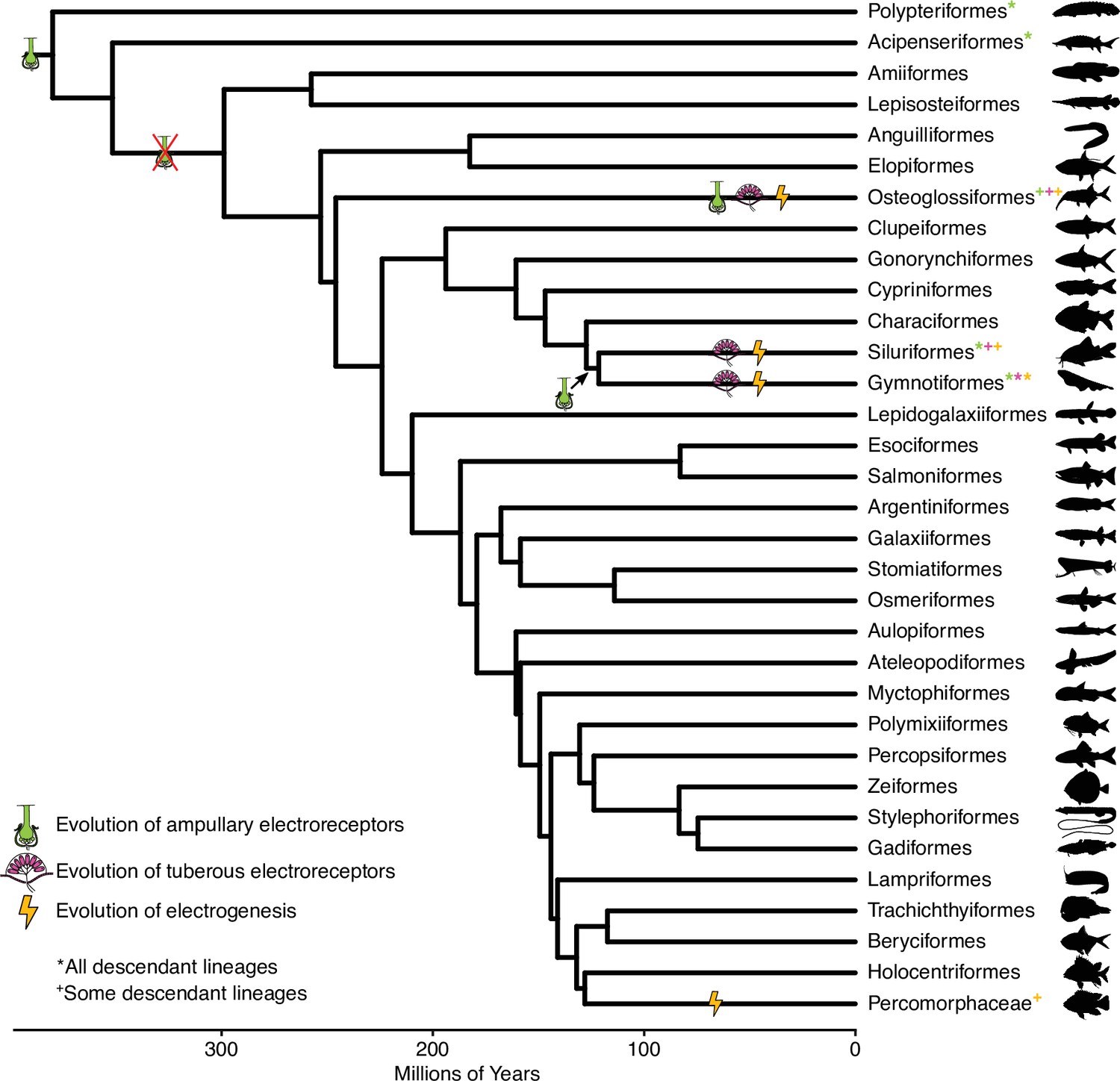
Chronogram of ray-finned fish orders, based on Hughes et al., 2018, showing the evolution of electrosensory phenotypes.
Symbols indicate independent origins of each electrosensory phenotype. * indicates all descendant lineages have that electrosensory phenotype while + indicates some descendant lineages have that electrosensory phenotype. Green, ampullary electroreceptors; magenta, tuberous electroreceptors; orange, electrogenesis.
© 2019, Various. Silhouettes are from http://phylopic.org/ and are available under CC BY 3.0, CC BY-SA 3.0, or CC BY-NC-SA 3.0 licenses. Reproduction of this figure must abide by the terms of these licenses. See Supplementary file 3 for individual image credits.
Figure 2 with 2 supplements
Brain morphology varies across species.
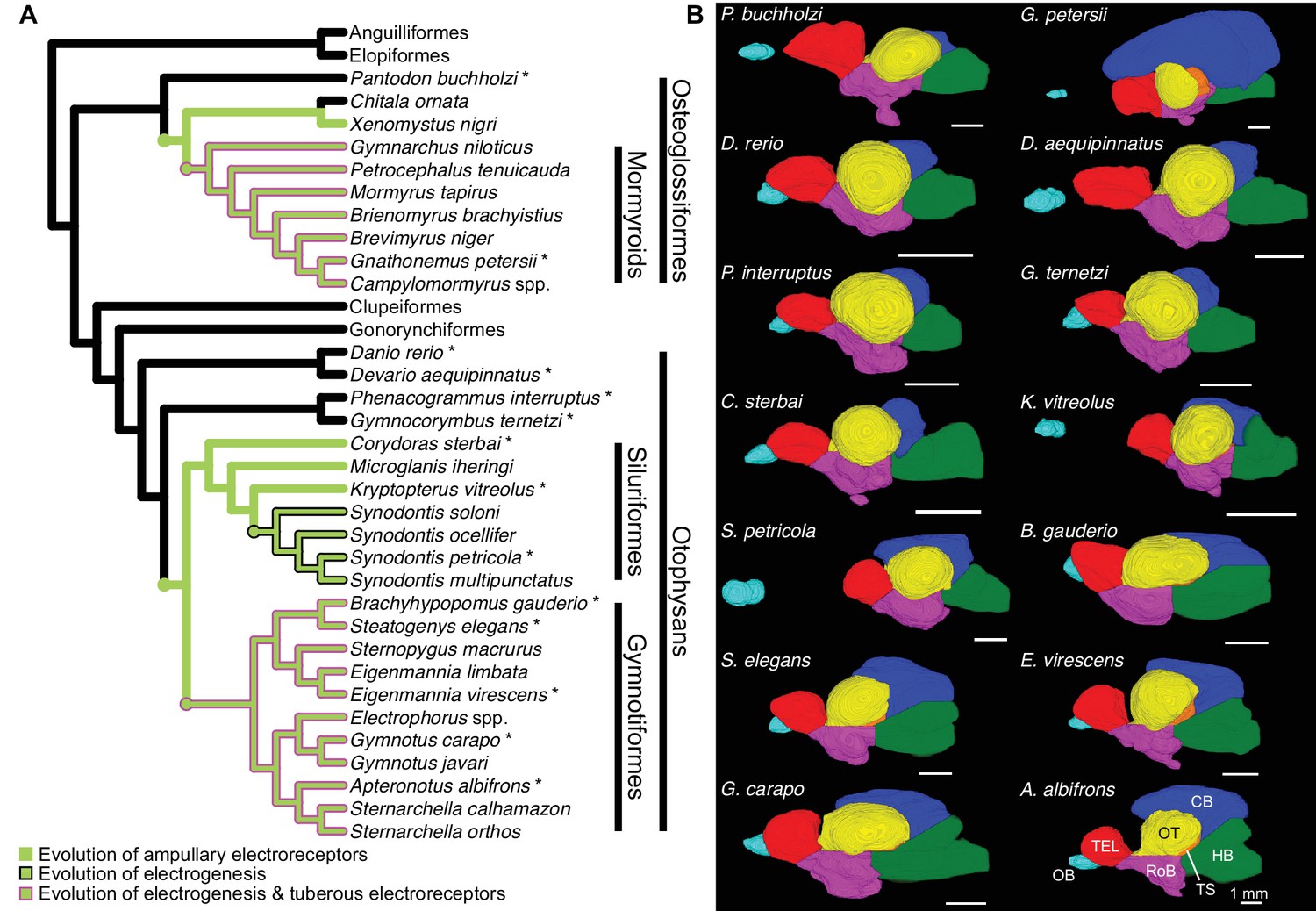
(A) Cladogram of the inferred phylogenetic relationships of species included in this study (N = 32) and the orders between them. Order level relationships are based on Hughes et al., 2018. Green branches represent presence of ampullary electroreceptors. Black outline represents electrogenic species while the magenta outline represents electrogenic species with tuberous electroreceptors. (B) Example 3D reconstructions of brains from this study; these species are indicated on the cladogram with an asterisk. Brains are oriented from a lateral view with anterior to the left and dorsal at the top. Brain regions are color coded: OB, olfactory bulbs (cyan); TEL, telencephalon (red); HB, hindbrain (green); OT, optic tectum (yellow); TS, torus semicircularis (orange); CB, cerebellum (blue); RoB, rest of brain (magenta). Scale bar = 1 mm.
Figure 2—figure supplement 1
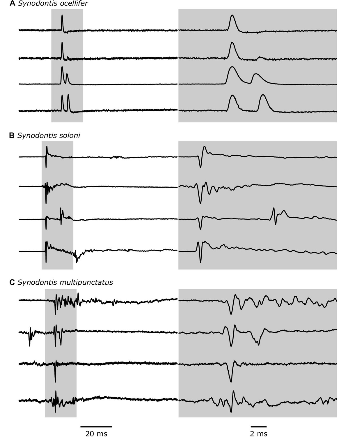
Electric discharges recorded from Synodontis spp.
Four example traces that highlight the diversity of recorded electric discharges for Synodontis ocellifer (A), Synodontis soloni (B), and Synodontis multipunctatus (C). The left column shows traces with a scale bar of 20 ms. The shaded gray area is shown in the right column at a shorter time scale (scale bar = 2 ms). Discharges are amplitude-normalized and oriented in the same direction, but head-positive polarity is unknown.
Figure 2—video 1
Example 3D reconstructions of brains from Figure 1B.
Brains are oriented from a lateral view with anterior to the left and dorsal at the top. Brain regions are color-coded: OB, olfactory bulbs (cyan); TEL, telencephalon (red); HB, hindbrain (green); OT, optic tectum (yellow); TS, torus semicircularis (orange); CB, cerebellum (blue); RoB, rest of brain (magenta). Scale bar = 1 mm.
Figure 3
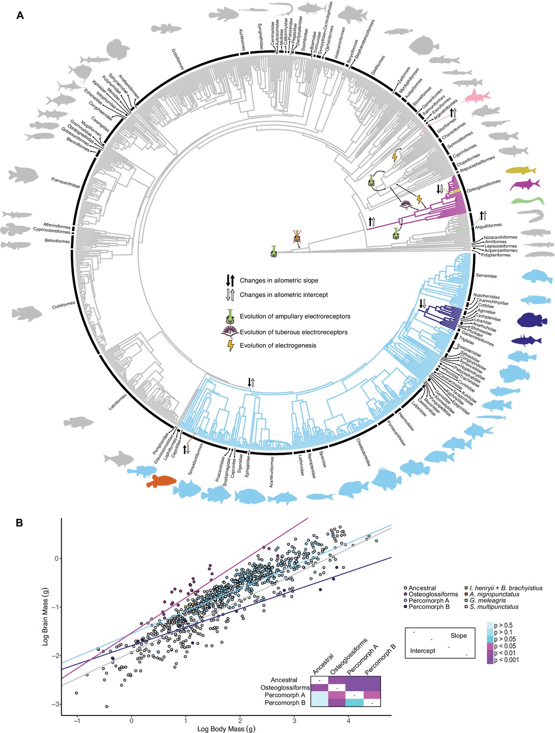
Mormyroids are more encephalized than gymnotiforms.
(A) Chronogram of ray-finned fishes based on Rabosky et al., 2018 showing shifts in the brain–body allometric relationship. Different branch colors indicate different allometric relationships. Direction of slope changes is indicated by black arrows, and direction of intercept changes is indicated by white arrows. Electrosensory phenotypes are indicated by symbols. Tree topology differs from the phylogenies in Figures 1–2, which highlights the well-established difficulty and discrepancies in resolving taxonomic relationships of ray-finned fishes. (B) Plot of log brain size by log body size. Points correspond to species means and are colored according to the identified grades in (A). Phylogenetic generalized least squares (PGLS) lines correspond to the distinct allometric relationships indicated in (A) and were determined for grades with at least three descendants. Inset shows a heatmap of the phylogenetically corrected pairwise post-hoc analysis of covariance (ANCOVA) results with a Bonferroni correction for differences in intercept below the diagonal and differences in slope above the diagonal. Significant differences are in shades of magenta/purple and nonsignificant differences are in shades of blue.
© 2019, Various. Silhouettes are from http://phylopic.org/ and are available under CC BY 3.0, CC BY-SA 3.0, or CC BY-NC-SA 3.0 licenses. Reproduction of this figure must abide by the terms of these licenses. See Supplementary file 3 for individual image credits.
-
Figure 3—source data 1
Ornstein–Uhlenbeck modeling (OUrjMCMC) and phylogenetic generalized least squares (PGLS) fitted brain–body allometries for each grade.
- https://cdn.elifesciences.org/articles/74159/elife-74159-fig3-data1-v2.xlsx
-
Figure 3—source data 2
Results (p-values) of phylogenetically corrected pairwise post-hoc tests with a Bonferroni correction for an analysis of covariance (ANCOVA) comparing phylogenetic generalized least squares (PGLS) relationships of brain size against body for each identified grade.
Differences in intercept are below the diagonal and differences in slope are above the diagonal. Significant differences are shown in bold.
- https://cdn.elifesciences.org/articles/74159/elife-74159-fig3-data2-v2.xlsx
-
Figure 3—source data 3
Model selection results for phylogenetic generalized least squares (PGLS) relationships systematically collapsing each putative grade to its ancestral grade.
The best-fit model is shown in bold.
- https://cdn.elifesciences.org/articles/74159/elife-74159-fig3-data3-v2.xlsx
-
Figure 3—source data 4
Ornstein–Uhlenbeck modeling (OUrjMCMC) estimated marginal likelihoods and model selection results for shifts in brain–body allometries associated with electrosensory phenotypes.
The best-fit model is shown in bold.
- https://cdn.elifesciences.org/articles/74159/elife-74159-fig3-data4-v2.xlsx
Figure 4 with 2 supplements
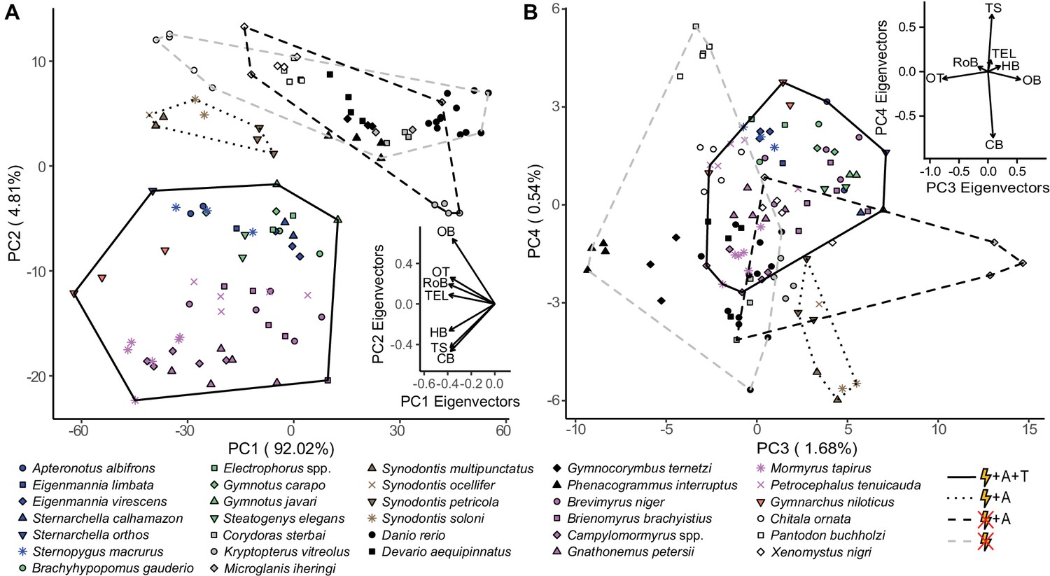
Species cluster distinctly in principal component (PC) space based on electrosensory phenotype.
Hindbrain, torus semicircularis, and cerebellum are loaded in the direction of electrogenic taxa for PC1 and PC2 (A), but not for PC3 and PC4 (B). Each point represents an individual, shapes correspond to species, and colors correspond to lineages: orange, wave mormyroid (N = 1); pink, pulse mormyroids (N = 6); white, outgroup osteoglossiforms (N = 3); blue, wave gymnotiforms (N = 6); green, pulse gymnotiforms (N = 5); brown, Synodontis siluriforms (N = 4); gray, non-electric siluriforms (N = 3); black, outgroup otophysans (N = 4). Minimum convex hulls correspond to electrosensory phenotypes: electrogenic + ampullary + tuberous electroreceptors (solid), electrogenic + only ampullary electroreceptors (dotted), only ampullary electroreceptors (black dashed), and non-electrosensory (gray dashed). Insets shows PC eigenvectors of each brain region. OB, olfactory bulbs; TEL, telencephalon; HB, hindbrain; OT, optic tectum; TS, torus semicircularis; CB, cerebellum; RoB, rest of brain.
-
Figure 4—source data 1
Phylogenetically corrected principal components analysis (pPCA) loadings for each non-normalized brain region.
OB, olfactory bulbs; TEL, telencephalon; HB, hindbrain; OT, optic tectum; TS, torus semicircularis; CB, cerebellum; RoB, rest of brain.
- https://cdn.elifesciences.org/articles/74159/elife-74159-fig4-data1-v2.xlsx
-
Figure 4—source data 2
Phylogenetically corrected principal components analysis (pPCA) phylogenetic generalized least squares (PGLS) model selection results for non-normalized data (N = 31).
PC1 was correlated with total brain volume, thus total brain volume was removed from all PC1 models. The best-fit model for each PC is shown in bold.
- https://cdn.elifesciences.org/articles/74159/elife-74159-fig4-data2-v2.xlsx
-
Figure 4—source data 3
Phylogenetic flexible discriminant analysis (pFDA) results table showing the regional coefficients for each discriminant axis and the means for each electrosensory phenotype group along each axis: electrogenic + tuberous and ampullary electroreceptors (E + A + T), electrogenic + only ampullary electroreceptors (E + A), and non-electric (Not E).
OB, olfactory bulbs; TEL, telencephalon; HB, hindbrain; OT, optic tectum; TS, torus semicircularis; CB, cerebellum; RoB, rest of brain.
- https://cdn.elifesciences.org/articles/74159/elife-74159-fig4-data3-v2.xlsx
Figure 4—figure supplement 1
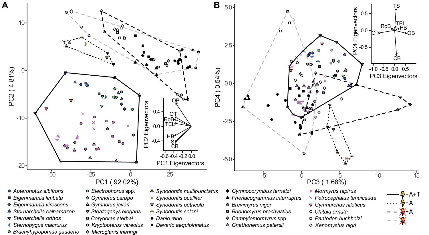
Species cluster distinctly in z-score normalized principal component (PC) space based on electrosensory phenotype.
Hindbrain, torus semicircularis, and cerebellum were loaded in the direction of electrogenic taxa for PC1 and PC2 (A), but not for PC3 and PC4 (B). Each point represents an individual, shapes correspond to species, and colors correspond to lineages: orange, wave mormyroid (N = 1); pink, pulse mormyroids (N = 6); white, outgroup osteoglossiforms (N = 3); blue, wave gymnotiforms (N = 6); green, pulse gymnotiforms (N = 5); brown, Synodontis siluriforms (N = 4); gray, non-electric siluriforms (N = 3); black, outgroup otophysans (N = 4). Minimum convex hulls correspond to electrosensory phenotypes: electrogenic + ampullary + tuberous electroreceptors (solid), electrogenic + only ampullary electroreceptors (dotted), only ampullary electroreceptors (black dashed), and non-electrosensory (gray dashed). Insets shows PC eigenvectors of each brain region. OB, olfactory bulbs; TEL, telencephalon; HB, hindbrain; OT, optic tectum; TS, torus semicircularis; CB, cerebellum; RoB, rest of brain.
Figure 4—figure supplement 2
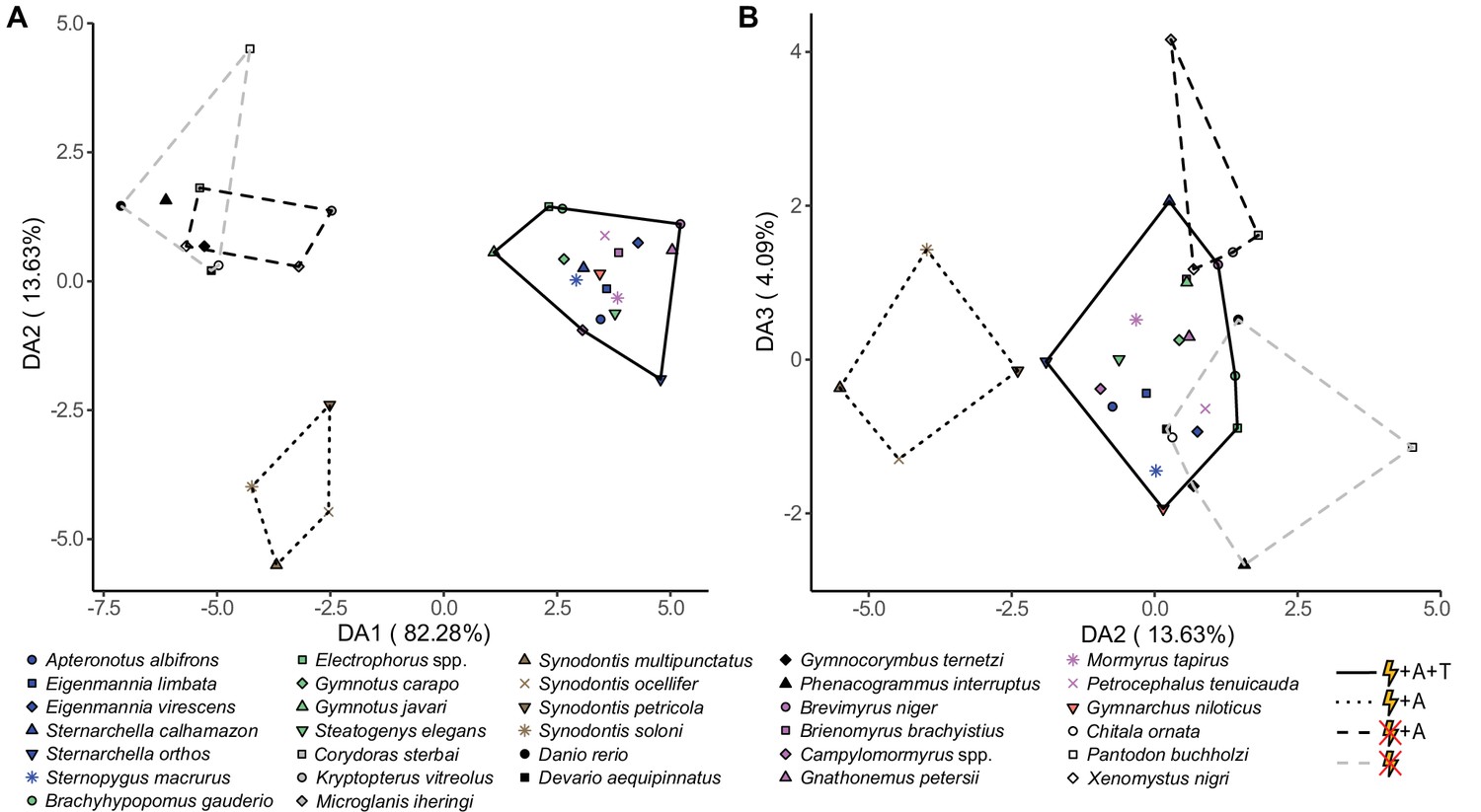
Species cluster distinctly in discriminant space based on electrosensory phenotype.
Points represent species means, shapes correspond to species, and colors correspond to lineages: orange, wave mormyroid (N = 1); pink, pulse mormyroids (N = 6); white, outgroup osteoglossiforms (N = 3); blue, wave gymnotiforms (N = 6); green, pulse gymnotiforms (N = 5); brown, Synodontis siluriforms (N = 4); gray, non-electric siluriforms (N = 3); black, outgroup otophysans (N = 4). Minimum convex hulls correspond to electrosensory phenotypes: electrogenic + ampullary + tuberous electroreceptors (solid), electrogenic + only ampullary electroreceptors (dotted), only ampullary electroreceptors (black dashed), and non-electrosensory (gray dashed).
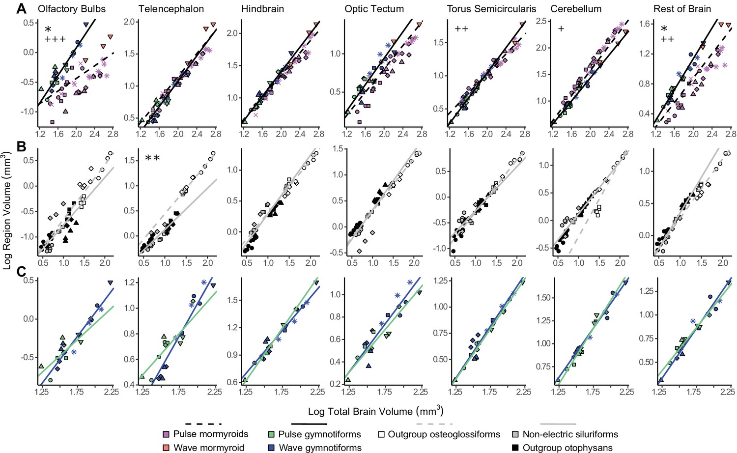
Figure 5 with 2 supplements

Mosaic increases in hindbrain, torus semicircularis, and cerebellum in electrogenic species with ampullary and tuberous electroreceptors.
Plots of log region volume against log total brain volume for olfactory bulbs (A), telencephalon (B), hindbrain (C), optic tectum (D), torus semicircularis (E), cerebellum (F), and rest of brain (G). Each point corresponds to an individual and shapes represent the same species as Figure 4. Phylogenetic generalized least squares (PGLS) lines were determined from species means and correspond to electrosensory phenotypes that cluster distinctly in Figure 4: electrogenic + ampullary + tuberous electroreceptors (pink, orange, green, blue points; solid line; N = 18), electrogenic + only ampullary electroreceptors (brown points; dotted line; N = 4), and non-electric (gray, white, black points; dashed line; N = 10). Inset shows a heatmap of the phylogenetically corrected pairwise post-hoc analysis of covariance (ANCOVA) results with a Bonferroni correction for differences in intercept below the diagonal and differences in slope above the diagonal for each brain region. Significant differences are in shades of magenta/purple, and nonsignificant differences are in shades of blue. Post-hoc tests were not performed when the ANCOVA revealed no significant differences (indicated by ‘n.s.’).
-
Figure 5—source data 1
Results of an analysis of covariance (ANCOVA) comparing phylogenetic generalized least squares (PGLS) relationships of region volume against total brain volume for each electrosensory phenotype: slope p, intercept p, and Pagel’s lambda (λ).
Significant differences are shown in bold. OB, olfactory bulbs; TEL, telencephalon; HB, hindbrain; OT, optic tectum; TS, torus semicircularis; CB, cerebellum; RoB, rest of brain.
- https://cdn.elifesciences.org/articles/74159/elife-74159-fig5-data1-v2.xlsx
-
Figure 5—source data 2
Results (p-values) of pairwise post-hoc tests with a Bonferroni correction for an analysis of covariance (ANCOVA) comparing phylogenetic generalized least squares (PGLS) relationships of region volume against total brain volume for each electrosensory phenotype: electrogenic + tuberous and ampullary electroreceptors (E + A + T), electrogenic + only ampullary electroreceptors (E + A), and non-electric (Not E).
Differences in intercept are below the diagonal, and differences in slope are above the diagonal for each brain region. Significant differences are shown in bold. Post-hoc tests were not performed when the ANCOVA revealed no significant differences (indicated by ‘n.s.’). OB, olfactory bulbs; TEL, telencephalon; HB, hindbrain; OT, optic tectum; TS, torus semicircularis; CB, cerebellum; RoB, rest of brain.
- https://cdn.elifesciences.org/articles/74159/elife-74159-fig5-data2-v2.xlsx
-
Figure 5—source data 3
Estimated effect sizes (Cohen’s d) of each contrast for an analysis of covariance (ANCOVA) comparing phylogenetic generalized least squares (PGLS) relationships of region volume against total brain volume for each electrosensory phenotype: electrogenic + tuberous and ampullary electroreceptors (E + A + T), electrogenic + only ampullary electroreceptors (E + A), and non-electric (Not E).
Post-hoc tests were not performed when the ANCOVA revealed no significant differences (indicated by ‘n.s.’). OB, olfactory bulbs; TEL, telencephalon; HB, hindbrain; OT, optic tectum; TS, torus semicircularis; CB, cerebellum; RoB, rest of brain.
- https://cdn.elifesciences.org/articles/74159/elife-74159-fig5-data3-v2.xlsx
-
Figure 5—source data 4
Results of an analysis of covariance (ANCOVA) comparing phylogenetic generalized least squares (PGLS) relationships of region volume against total brain–region volume for each electrosensory phenotype: slope p, intercept p, and Pagel’s lambda (λ).
Significant differences are shown in bold. OB, olfactory bulbs; TEL, telencephalon; HB, hindbrain; OT, optic tectum; TS, torus semicircularis; CB, cerebellum; RoB, rest of brain.
- https://cdn.elifesciences.org/articles/74159/elife-74159-fig5-data4-v2.xlsx
-
Figure 5—source data 5
Results (p-values) of pairwise post-hoc tests with a Bonferroni correction for an analysis of covariance (ANCOVA) comparing phylogenetic generalized least squares (PGLS) relationships of region volume against total brain–region volume for each electrosensory phenotype: electrogenic + tuberous and ampullary electroreceptors (E + A + T), electrogenic + only ampullary electroreceptors (E + A), and non-electric (Not E).
Differences in intercept are below the diagonal, and differences in slope are above the diagonal for each brain region. Significant differences are shown in bold. Post-hoc tests were not performed when the ANCOVA revealed no significant differences (indicated by ‘n.s.’). OB, olfactory bulbs; TEL, telencephalon; HB, hindbrain; OT, optic tectum; TS, torus semicircularis; CB, cerebellum; RoB, rest of brain.
- https://cdn.elifesciences.org/articles/74159/elife-74159-fig5-data5-v2.xlsx
-
Figure 5—source data 6
Estimated effect sizes (Cohen’s d) of each contrast for an analysis of covariance (ANCOVA) comparing phylogenetic generalized least squares (PGLS) relationships of region volume against total brain–region volume for each electrosensory phenotype: electrogenic + tuberous and ampullary electroreceptors (E + A + T), electrogenic + only ampullary electroreceptors (E + A), and non-electric (Not E).
Post-hoc tests were not performed when the ANCOVA revealed no significant differences (indicated by ‘n.s.’). OB, olfactory bulbs; TEL, telencephalon; HB, hindbrain; OT, optic tectum; TS, torus semicircularis; CB, cerebellum; RoB, rest of brain.
- https://cdn.elifesciences.org/articles/74159/elife-74159-fig5-data6-v2.xlsx
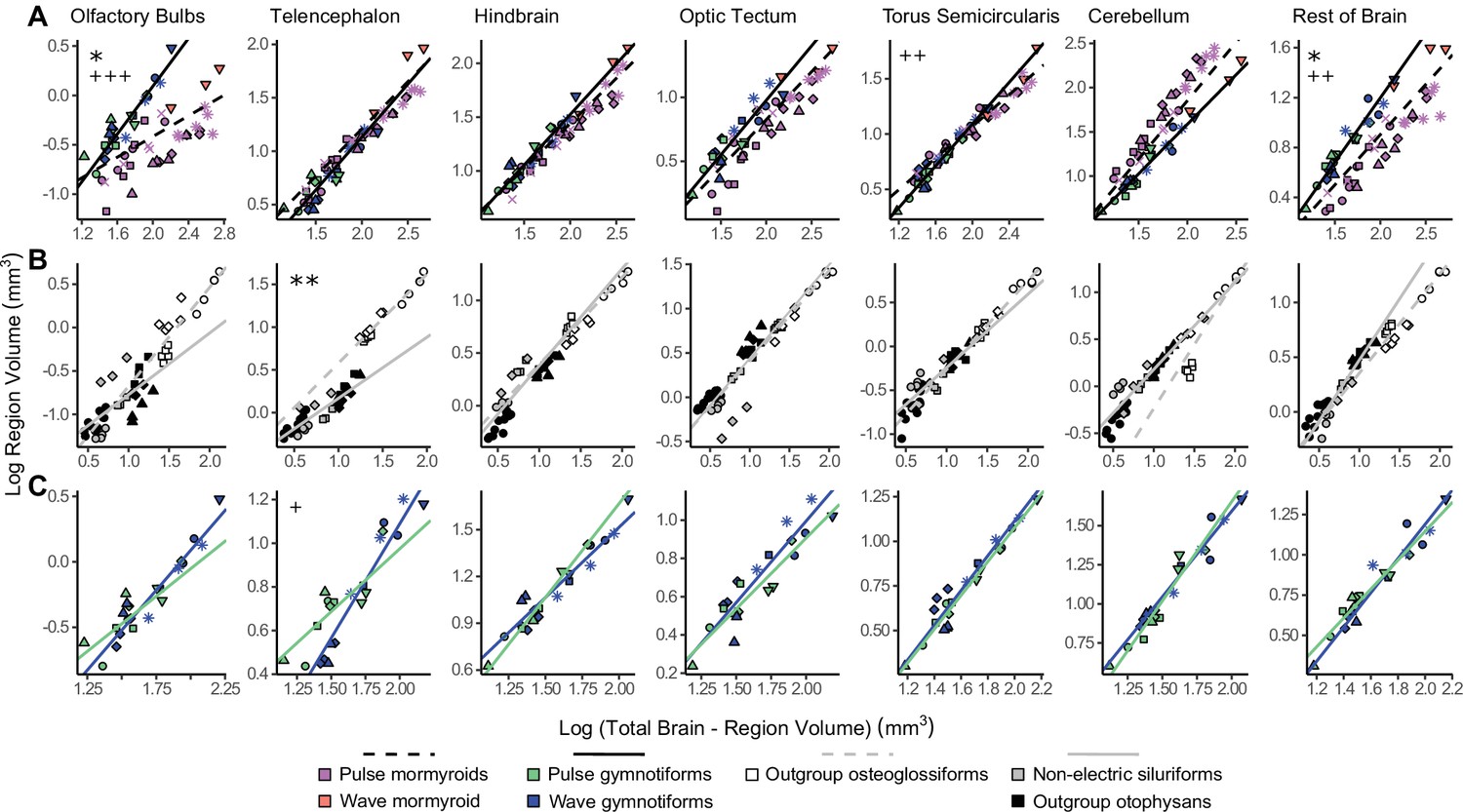
Figure 5—figure supplement 1

Apparent mosaic shifts in olfactory bulbs, hindbrain, optic tectum, torus semicircularis, cerebellum, and rest of brain between electrogenic species with ampullary and tuberous electroreceptors and non-electric species.
Plots of log region volume against log total brain–region volume for olfactory bulbs (A), telencephalon (B), hindbrain (C), optic tectum (D), torus semicircularis (E), cerebellum (F), and rest of brain (G). Each point corresponds to an individual and shapes represent the same species as Figure 4. Phylogenetic generalized least squares (PGLS) lines were determined from species means and correspond to electrosensory phenotypes that cluster distinctly in Figure 4: electrogenic + tuberous and ampullary electroreceptors (pink, orange, green, blue points; solid line; N = 18), electrogenic + only ampullary electroreceptors (brown points; dotted line; N = 4), and non-electric (gray, white, black points; dashed line; N = 10). Inset shows a heatmap of the phylogenetically corrected pairwise post-hoc ANCOVA results with a Bonferroni correction for differences in intercept below the diagonal and differences in slope above the diagonal for each brain region. Significant differences are in shades of magenta/purple, and nonsignificant differences are in shades of blue. Post-hoc tests were not performed when the ANCOVA revealed no significant differences (indicated by ‘n.s.’).
Figure 5—figure supplement 2
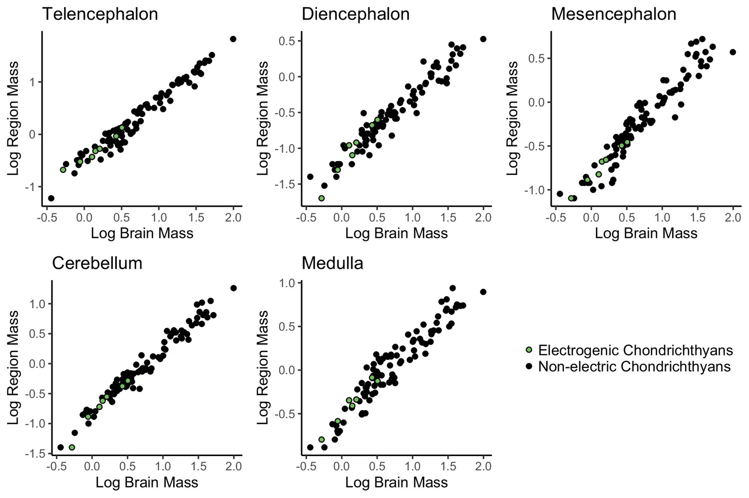
No evidence of mosaic shifts in cerebellum or medulla of electrogenic chondrichthyans.
Plots of log region mass against total brain mass, data from Mull et al., 2020. Each point is a species, electrogenic taxa are in green, and non-electric taxa are in black.
Figure 6
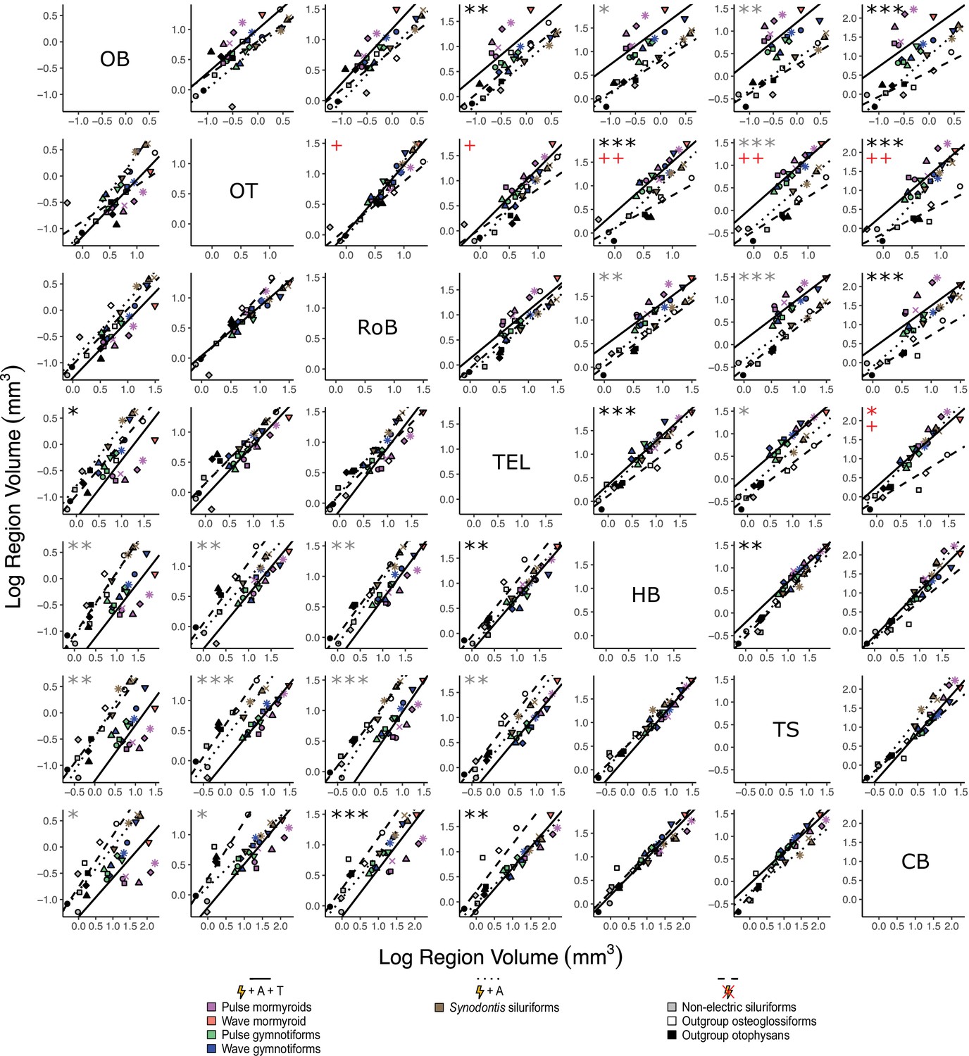
Matrix of scatterplots for each region-by-region comparison.
Columns indicate the region on the y-axis, and rows indicate the region on the x-axis. Points correspond to species means, and shapes represent the same species as Figure 4. Phylogenetic generalized least squares (PGLS) lines were determined from species means and correspond to electrosensory phenotypes that cluster distinctly in Figure 4: electrogenic + tuberous and ampullary electroreceptors (pink, orange, green, blue points; solid line; N = 18), electrogenic + only ampullary electroreceptors (brown points; dotted line; N = 4), and non-electric (gray, white, black points; dashed line; N = 10). Significant differences in intercept are marked with asterisks: *p<0.05, **p<0.01. Significant differences in slope are marked with pluses: +p<0.05, ++p<0.01, +++p<0.001. Significant differences between electrogenic + tuberous and ampullary electroreceptors taxa and non-electric taxa are marked in black. Significant differences between tuberous receptor taxa (E + A + T) and taxa lacking tuberous receptors (E + A and not E) are marked in gray. Significant differences between all electrogenic taxa (E + A + T and E + A) and non-electric taxa are marked in red. OB, olfactory bulbs; TEL, telencephalon; HB, hindbrain; OT, optic tectum; TS, torus semicircularis; CB, cerebellum; RoB, rest of brain.
-
Figure 6—source data 1
Matrix of region-by-region analysis of covariance (ANCOVA) results comparing phylogenetic generalized least squares (PGLS) relationships for each electrosensory phenotype: slope p (S), intercept p (I), and Pagel’s lambda (L).
Columns indicate the region on the y-axis, and rows indicate the region on the x-axis. Significant differences are shown in bold. OB, olfactory bulbs; TEL, telencephalon; HB, hindbrain; OT, optic tectum; TS, torus semicircularis; CB, cerebellum; RoB, rest of brain.
- https://cdn.elifesciences.org/articles/74159/elife-74159-fig6-data1-v2.xlsx
-
Figure 6—source data 2
Matrix of region-by-region analysis of covariance (ANCOVA) results comparing phylogenetic generalized least squares (PGLS) relationships for each electrosensory phenotype: electrogenic + tuberous and ampullary electroreceptors (E + A + T), electrogenic + only ampullary electroreceptors (E + A), and non-electric (Not E).
Columns indicate the region on the y-axis, and rows indicate the region on the x-axis. Numbers in each matrix cell are the results (p-values) of pairwise post-hoc tests with a Bonferroni correction. Differences in intercept are below the diagonal, and differences in slope are above the diagonal for each inset. Significant differences are shown in bold. Post-hoc tests were not performed when the ANCOVA revealed no significant differences (indicated by ‘n.s.’). OB, olfactory bulbs; TEL, telencephalon; HB, hindbrain; OT, optic tectum; TS, torus semicircularis; CB, cerebellum; RoB, rest of brain.
- https://cdn.elifesciences.org/articles/74159/elife-74159-fig6-data2-v2.xlsx
-
Figure 6—source data 3
Matrix of region-by-region analysis of covariance (ANCOVA) results comparing phylogenetic generalized least squares (PGLS) relationships for each electrosensory phenotype: electrogenic + tuberous and ampullary electroreceptors (E + A + T), electrogenic + only ampullary electroreceptors (E + A), and non-electric (Not E).
Columns indicate the region on the y-axis, and rows indicate the region on the x-axis. Numbers in each matrix cell are the estimated effect sizes (Cohen’s d) of each contrast. Post-hoc tests were not performed when the ANCOVA revealed no significant differences (indicated by ‘n.s.’). OB, olfactory bulbs; TEL, telencephalon; HB, hindbrain; OT, optic tectum; TS, torus semicircularis; CB, cerebellum; RoB, rest of brain.
- https://cdn.elifesciences.org/articles/74159/elife-74159-fig6-data3-v2.xlsx
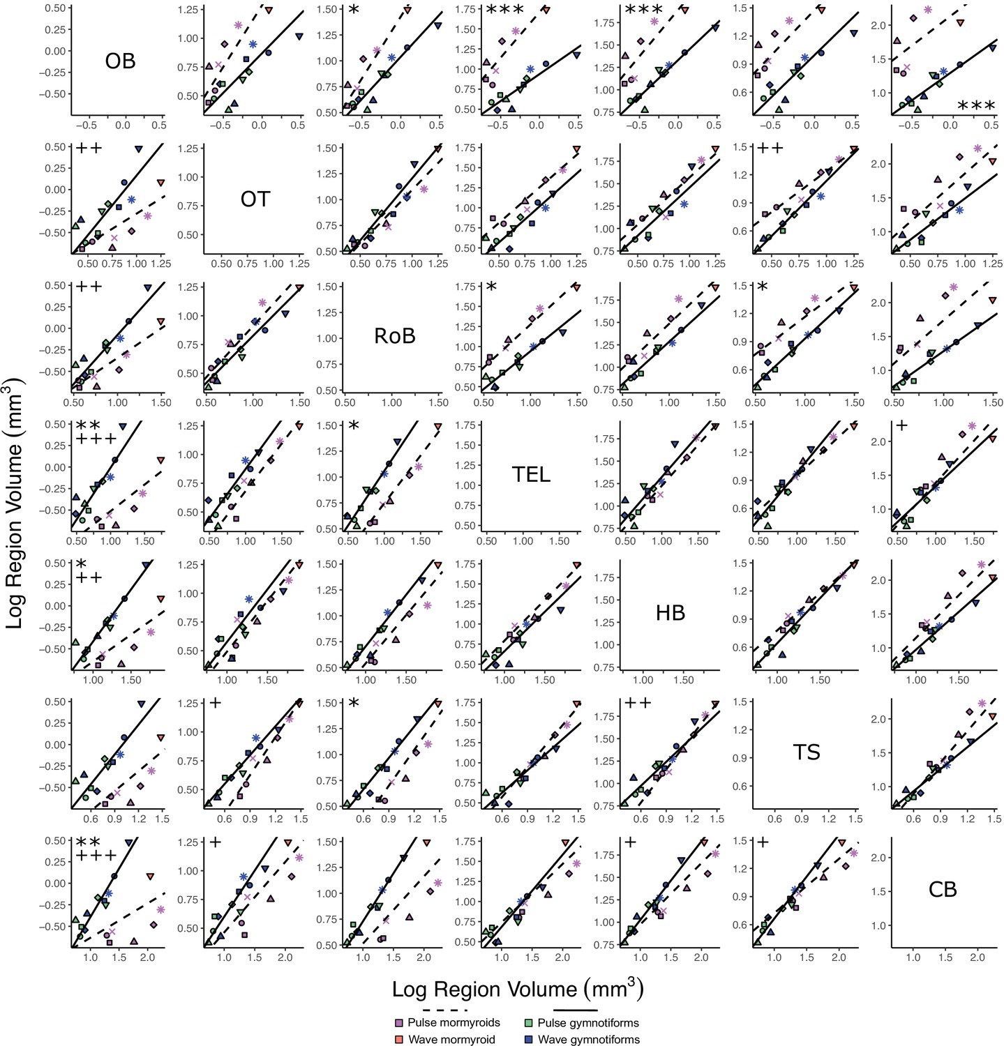
Figure 7 with 4 supplements
Lineage-specific mosaic shifts within phenotypes in olfactory bulbs, telencephalon, and rest of brain.
Plots of log brain region volumes by log total brain volume for (A) mormyroids (pink and orange points, dashed black lines, N = 7) vs. gymnotiforms (blue and green points, solid black line, N = 11); (B) non-electric osteoglossiforms (white points, dashed gray line, N = 3) vs. non-electric otophysans (gray and black points, solid gray line, N = 7); and (C) wave (blue, N = 6) vs. pulse (green, N = 5) gymnotiforms. Each point corresponds to an individual, and shapes represent the same species as Figure 4. Phylogenetic generalized least squares (PGLS) lines were determined from species means and compared using phylogenetically corrected analysis of covariances (ANCOVAs). Significant differences in intercept are marked with asterisks: *p<0.05, **p<0.01. Significant differences in slope are marked with pluses: +p<0.05, ++p<0.01, +++p<0.001.
-
Figure 7—source data 1
Lineage analysis of covariance (ANCOVA) results comparing phylogenetic generalized least squares (PGLS) relationships of region volume against total brain volume for each lineage: slope p, intercept p, Pagel’s lambda (λ), Cohen’s d.
Significant differences are shown in bold. OB, olfactory bulbs; TEL, telencephalon; HB, hindbrain; OT, optic tectum; TS, torus semicircularis; CB, cerebellum; RoB, rest of brain.
- https://cdn.elifesciences.org/articles/74159/elife-74159-fig7-data1-v2.xlsx
-
Figure 7—source data 2
Lineage analysis of covariance (ANCOVA) results comparing phylogenetic generalized least squares (PGLS) relationships of region volume against total brain–region volume for each lineage: slope p, intercept p, Pagel’s lambda (λ), Cohen’s d.
Significant differences are shown in bold. OB, olfactory bulbs; TEL, telencephalon; HB, hindbrain; OT, optic tectum; TS, torus semicircularis; CB, cerebellum; RoB, rest of brain.
- https://cdn.elifesciences.org/articles/74159/elife-74159-fig7-data2-v2.xlsx
-
Figure 7—source data 3
Matrix of region-by-region analysis of covariance (ANCOVA) results comparing phylogenetic generalized least squares (PGLS) relationships for mormyroids vs. gymnotiforms: slope p (S), intercept p (I), Pagel’s lambda (L), and Cohen’s d (D).
Columns indicate the region on the y-axis, and rows indicate the region on the x-axis. Significant differences are shown in bold. OB, olfactory bulbs; TEL, telencephalon; HB, hindbrain; OT, optic tectum; TS, torus semicircularis; CB, cerebellum; RoB, rest of brain.
- https://cdn.elifesciences.org/articles/74159/elife-74159-fig7-data3-v2.xlsx
-
Figure 7—source data 4
Matrix of region-by-region analysis of covariance (ANCOVA) results comparing phylogenetic generalized least squares (PGLS) relationships for non-electric osteoglossiforms vs. non-electric otophysans: slope p (S), intercept p (I), Pagel’s lambda (L), and Cohen’s d (D).
Columns indicate the region on the y-axis, and rows indicate the region on the x-axis. Significant differences are shown in bold. OB, olfactory bulbs; TEL, telencephalon; HB, hindbrain; OT, optic tectum; TS, torus semicircularis; CB, cerebellum; RoB, rest of brain.
- https://cdn.elifesciences.org/articles/74159/elife-74159-fig7-data4-v2.xlsx
-
Figure 7—source data 5
Matrix of region-by-region analysis of covariance (ANCOVA) results comparing phylogenetic generalized least squares (PGLS) relationships for wave vs. pulse gymnotiforms: slope p (S), intercept p (I), Pagel’s lambda (L), and Cohen’s d (D).
Columns indicate the region on the y-axis, and rows indicate the region on the x-axis. Significant differences are shown in bold. OB, olfactory bulbs; TEL, telencephalon; HB, hindbrain; OT, optic tectum; TS, torus semicircularis; CB, cerebellum; RoB, rest of brain.
- https://cdn.elifesciences.org/articles/74159/elife-74159-fig7-data5-v2.xlsx
Figure 7—figure supplement 1
Lineage-specific mosaic shifts within phenotypes in olfactory bulbs, telencephalon, and rest of brain.
Plots of log brain region volumes by log total brain–region volume for (A) mormyroids (pink and orange points, dashed black lines, N = 7) vs. gymnotiforms (blue and green points, solid black line, N = 11); (B) non-electric osteoglossiforms (white points, dashed gray line, N = 3) vs. non-electric otophysans (gray and black points, solid gray line, N = 7); and (C) wave (blue, N = 6) vs. pulse (green, N = 5) gymnotiforms. Each point corresponds to an individual, and shapes represent the same species as Figure 4. Phylogenetic generalized least squares (PGLS) lines were determined from species means and compared using analysis of covariances (ANCOVAs). Significant differences in intercept are marked with asterisks: *p<0.05, **p<0.01. Significant differences in slope are marked with pluses: +p<0.05, ++p<0.01, +++p<0.001.
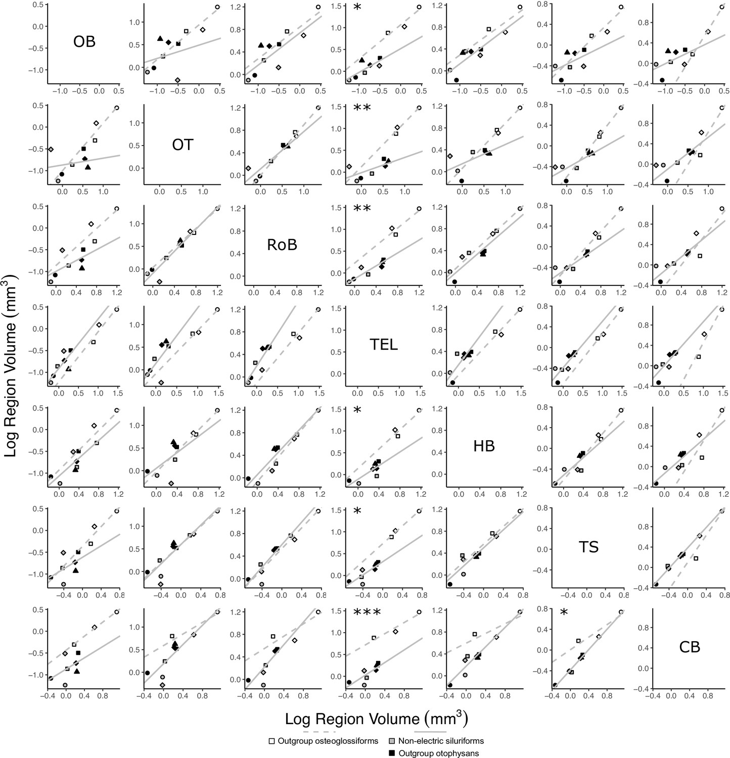
Figure 7—figure supplement 2
Matrix of scatterplots for each region-by-region comparison for mormyroids (pink and orange points, dashed black lines, N = 7) vs. gymnotiforms (blue and green points, solid black line, N = 11).
Columns indicate the region on the y-axis, and rows indicate the region on the x-axis. Points correspond to species means, and shapes represent the same species as Figure 4. Phylogenetic generalized least squares (PGLS) lines were determined from species means. Significant differences in intercept are marked with asterisks: *p<0.05, **p<0.01, ***p<0.001. Significant differences in slope are marked with pluses: +p<0.05, ++p<0.01, +++p<0.001.
Figure 7—figure supplement 3
Matrix of scatterplots for each region-by-region comparison for non-electric osteoglossiforms (white points, dashed gray line, N = 3) vs. non-electric otophysans (gray and black points, solid gray line, N = 7).
Columns indicate the region on the y-axis, and rows indicate the region on the x-axis. Points correspond to species means, and shapes represent the same species as Figure 4. Phylogenetic generalized least squares (PGLS) lines were determined from species means. Significant differences in intercept are marked with asterisks: *p<0.05, **p<0.01, ***p<0.001. There were no significant differences in slope.
Figure 7—figure supplement 4
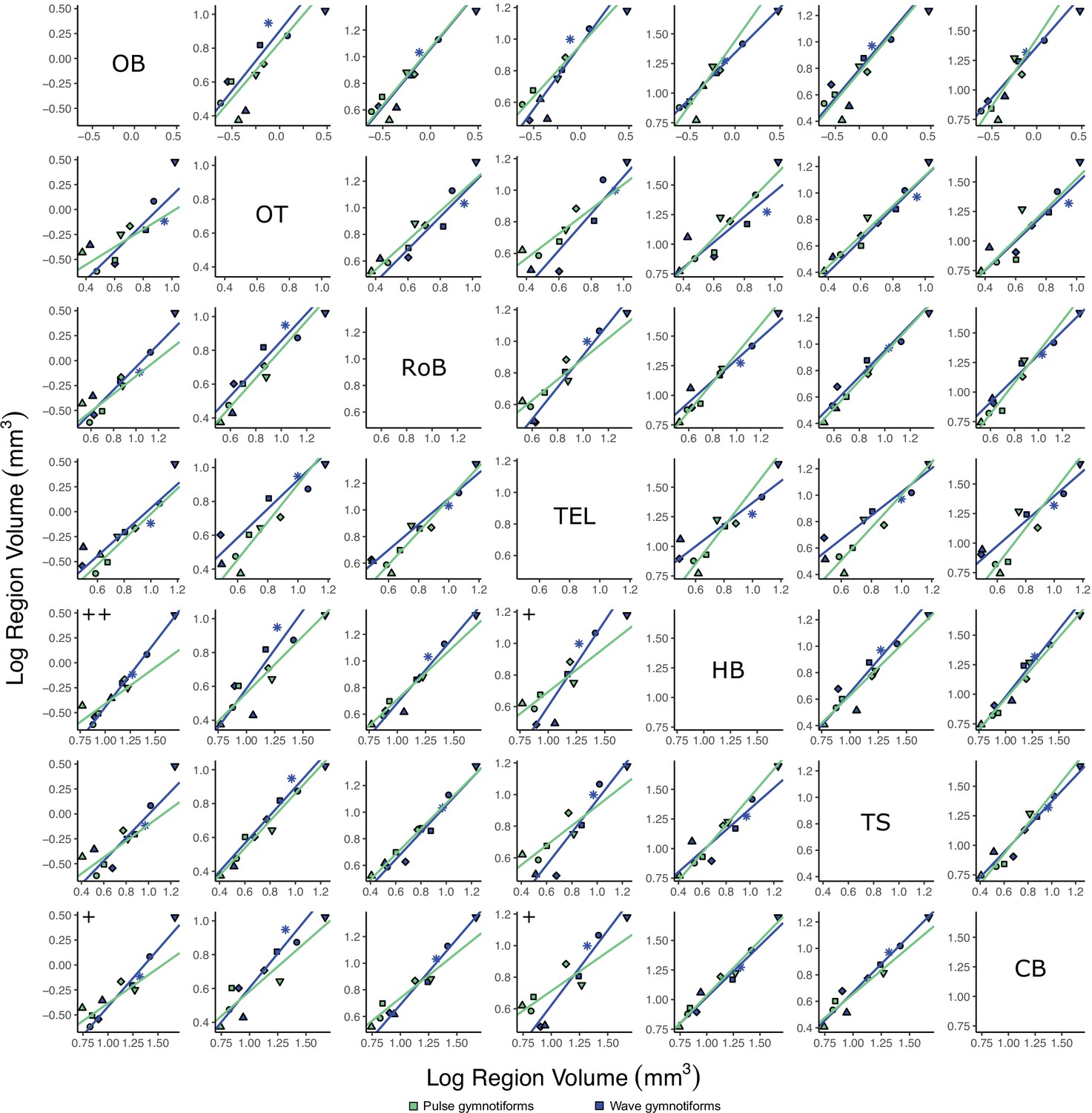
Matrix of scatterplots for each region-by-region comparison for wave (blue, N = 6) vs. pulse (green, N = 5) gymnotiforms.
Columns indicate the region on the y-axis, and rows indicate the region on the x-axis. Points correspond to species means, and shapes represent the same species as Figure 4. Phylogenetic generalized least squares (PGLS) lines were determined from species means. Significant differences in slope are marked with pluses: +p<0.05, ++p<0.01, +++p<0.001. There were no significant differences in intercept.
Figure 8
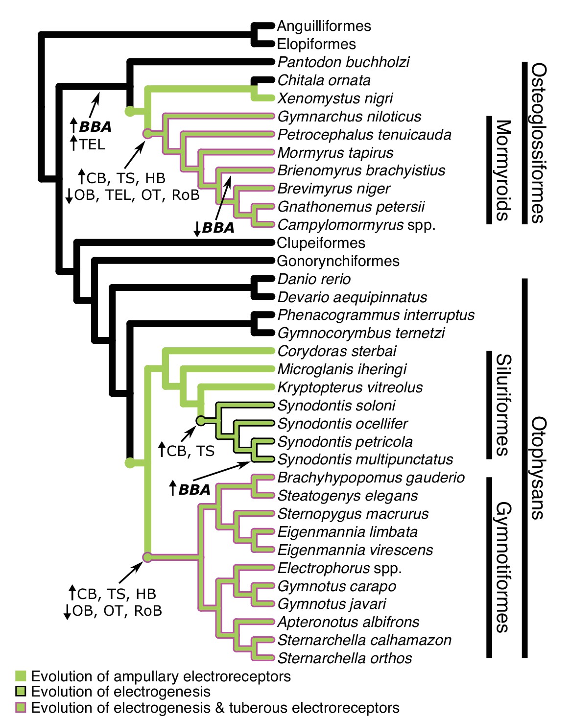
Cladogram of the inferred phylogenetic relationships of species included in this study (N = 32) and the orders between them depicting where shifts in brain–body allometries (indicated in bold italics) and relative mosaic shifts in region–brain allometries likely occurred.
Order level relationships are based on Hughes et al., 2018. Green branches represent presence of ampullary electroreceptors. Black outline represents electrogenic species while the magenta outline represents electrogenic species with tuberous electroreceptors. BBA, brain body allometry; OB, olfactory bulbs; TEL, telencephalon; HB, hindbrain; OT, optic tectum; TS, torus semicircularis; CB, cerebellum; RoB, rest of brain.
Figure 9
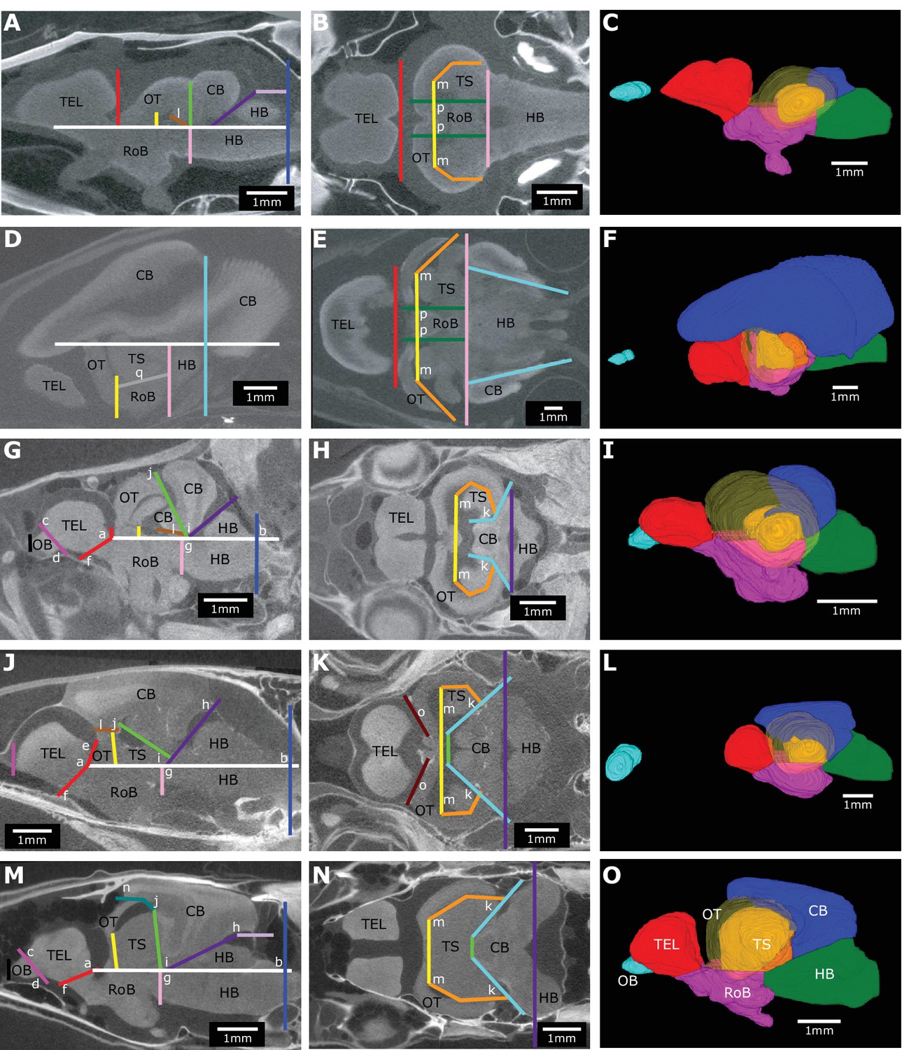
Brain landmarks and planes used to consistently delineate brain regions across species.
Example brain slices and 3D reconstructions from Pantodon buchholzi (A–C), Gnathonemus petersii (D–F), Phenocogrammus interruptus (G–I), Synodontis petricola (J–L), and Eigenmannia virescens (M–O) that show the landmarks (letters) and planes (lines). Osteoglossiform brain slices (A, B, E) were modified from Sukhum et al., 2018. Brain slices are oriented facing left in a sagittal plane (A, D, G, J, M) and horizontal plane (B, E, H, K, N). Images were made by averaging across 10 adjacent slices (A, B, E) or 5 adjacent slices (D, G, H, J, K, M, N). 3D reconstructions have a semi-transparent optic tectum to show the torus semicircularis. Brain regions are color-coded: OB, olfactory bulbs (cyan); TEL, telencephalon (red); HB, hindbrain (green); OT, optic tectum (yellow); TS, torus semicircularis (orange); CB, cerebellum (blue); RoB, rest of brain (magenta). Scale bar = 1 mm.
-
Figure 9—source data 1
Coefficient of variation results of repeated measures (N = 3) for four different brains.
OB, olfactory bulbs; TEL, telencephalon; HB, hindbrain; OT, optic tectum; TS, torus semicircularis; CB, cerebellum; RoB, rest of brain, TBV, total brain volume.
- https://cdn.elifesciences.org/articles/74159/elife-74159-fig9-data1-v2.xlsx
Additional files
-
Transparent reporting form
- https://cdn.elifesciences.org/articles/74159/elife-74159-transrepform1-v2.pdf
-
Supplementary file 1
Brain region data from this study.
OB, olfactory bulbs; TEL, telencephalon; HB, hindbrain; OT, optic tectum; TS, torus semicircularis; CB, cerebellum; RoB, rest of brain.
- https://cdn.elifesciences.org/articles/74159/elife-74159-supp1-v2.csv
-
Supplementary file 2
Ray-finned fishes brain and body mass data used in this study.
- https://cdn.elifesciences.org/articles/74159/elife-74159-supp2-v2.csv
-
Supplementary file 3
- https://cdn.elifesciences.org/articles/74159/elife-74159-supp3-v2.xlsx
Download links
A two-part list of links to download the article, or parts of the article, in various formats.
Downloads (link to download the article as PDF)
Open citations (links to open the citations from this article in various online reference manager services)
Cite this article (links to download the citations from this article in formats compatible with various reference manager tools)
Convergent mosaic brain evolution is associated with the evolution of novel electrosensory systems in teleost fishes
eLife 11:e74159.
https://doi.org/10.7554/eLife.74159


