The individuality of shape asymmetries of the human cerebral cortex
- Turner Institute for Brain and Mental Health, School of Psychological Sciences, Monash University, Australia
- Monash Biomedical Imaging, Monash University, Australia
- Monash Data Futures Institute, Monash University, Australia
- Healthy Brain and Mind Research Centre, Faculty of Health Sciences, Australian Catholic University, Australia
- Department of Psychology, Yale University, United States
- BrainPark, Turner Institute for Brain and Mental Health, School of Psychological Sciences, Monash University, Australia
- School of Physics, University of Sydney, Australia
- Center of Excellence for Integrative Brain Function, University of Sydney, Australia
- BrainKey Inc, United States
Figures
Figure 1 with 1 supplement
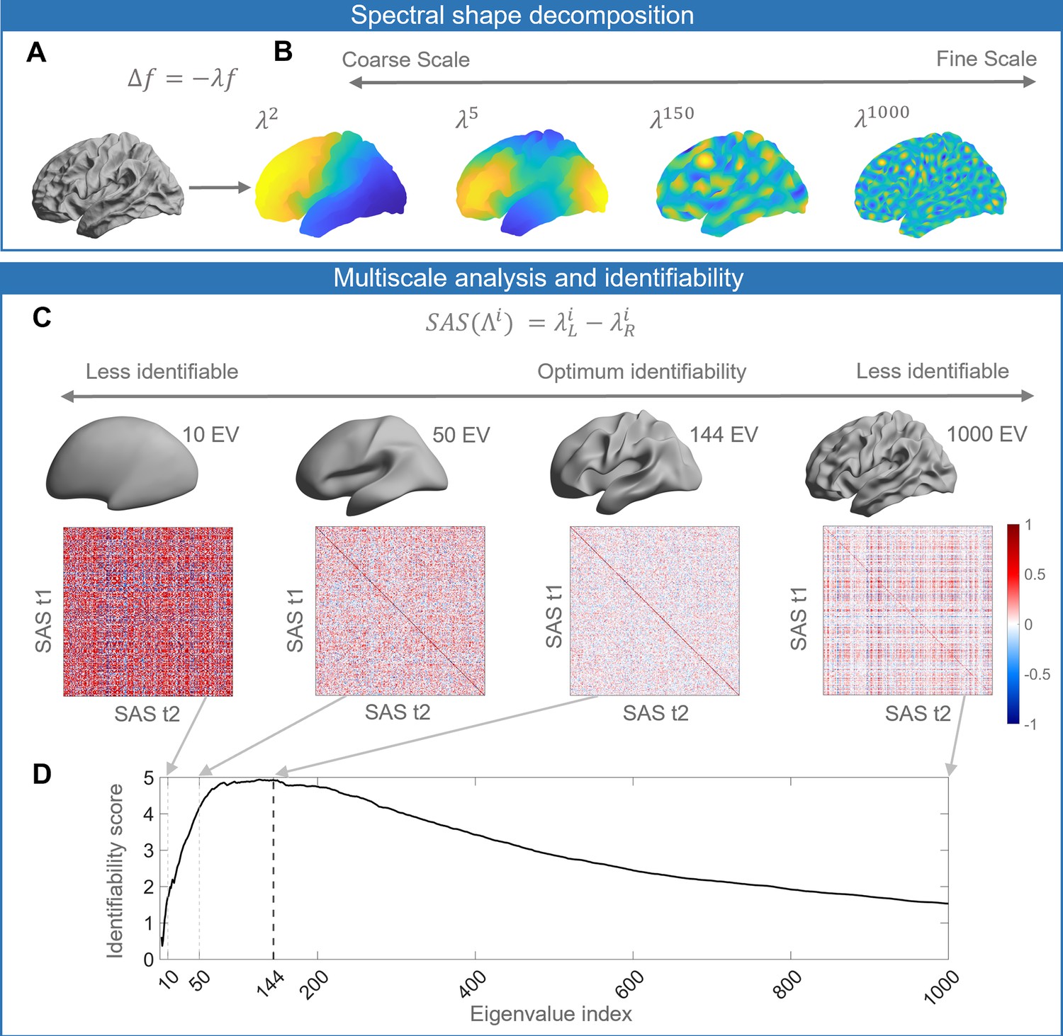
Schematic of our analysis workflow.
(A) The shapes of the left and right hemispheres are independently analyzed using the Laplace–Beltrami operator (LBO) via the Shape-DNA algorithm (Reuter et al., 2009; Reuter et al., 2006). (B) Eigenfunctions of the LBO are obtained by solving the Helmholtz equation on the surface, given by , where corresponds to a distinct eigenfunction, and is the corresponding eigenvalue. Each eigenvalue , quantifies the degree to which a given eigenfunction is expressed in the intrinsic geometry of the cortex. Higher-order eigenvalues describe shape variations at finer spatial scales. (C) The shape asymmetry signature (SAS) is quantified as the difference in the left and right hemisphere eigenvalue spectra, providing a summary measure of multiscale cortical shape asymmetries. To investigate the identifiability of the SAS, we use Pearson’s correlation to calculate the similarity between the SAS vectors obtained for the time 1 (t1) and time 2 (t2) two scans from the same individuals (diagonal elements of the matrices) as well as the correlation between t1 and t2 scans between different subjects (off-diagonal elements). We estimate identifiability by first correlating the initial two eigenvalues, then the initial three eigenvalues, and so on to a maximum of 1000 eigenvalues. Here, we show examples of correlation matrices obtained when using the first 10, 50, 144, and 1000 eigenvalues, and the cortical surface reconstructions show the shape variations captured by corresponding spatial scales. (D) Repeating the identifiability analysis up to a maximum of 1000 eigenvalues yields a curve with a clear peak, representing the scale at which individual differences in cortical shape are maximal. For the SAS, this peak occurs when the first 144 eigenvalues are used (black dashed line), which offers a fairly coarse description of shape variations (see panel C). We then use a similar analysis approach to investigate associations between scale-specific shape variations and sex, handedness, cognitive functions, as well as heritability. The data in this figure are from the OASIS-3 (n = 233) cohort, and the cortical surfaces are from a population-based template (fsaverage in FreeSurfer).
Figure 1—figure supplement 1
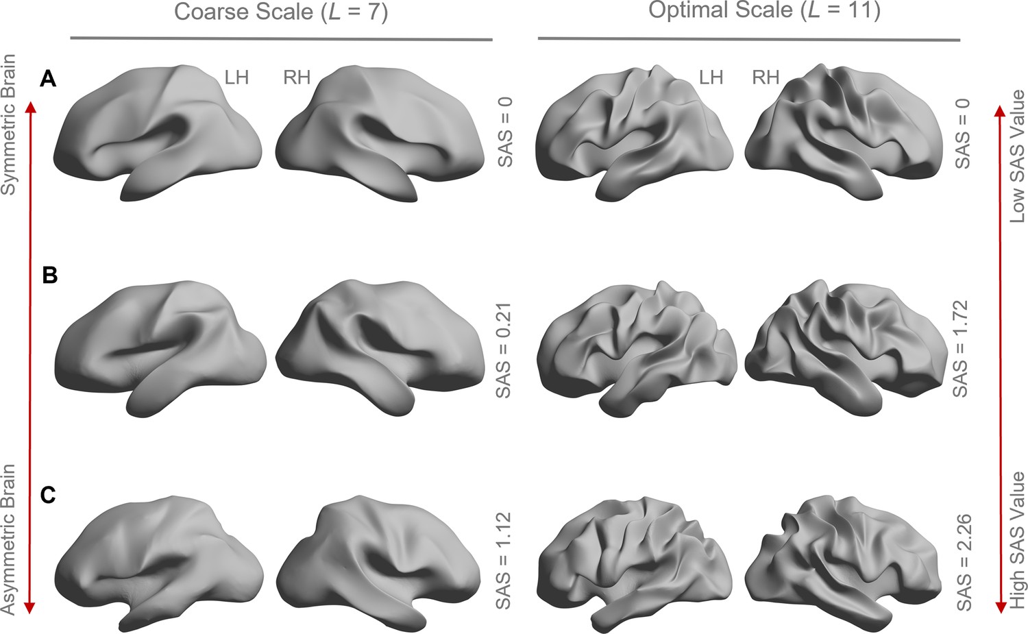
Higher shape asymmetry signature (SAS) values characterize brains with stronger cortical shape asymmetries.
Panels (A–C) show left and right cortical surface reconstructions for three individuals showing varying levels of the SAS, from perfectly symmetric (A) to highly asymmetric (C). The left panel shows reconstructions at a coarse spatial scale corresponding to the first seven eigengroups with a wavelength of about 55 mm. The right panel shows a reconstruction at the optimal scale for SAS identifiability, corresponding to the first 11 eigengroups and a wavelength of about 37 mm. The perfectly symmetric brain in panel (A) was created by projecting the left hemisphere to the right hemisphere using the population-based template (fsaverage). The SAS value is zero for this case. The surfaces in panels (B) and (C) correspond to individual participants with moderate (B) and strong (C) asymmetry. The gradations of asymmetry can be appreciated visually. As expected, the participant in panel (C) has a higher SAS than the participant in panel (B). The SAS values shown here are the absolute mean values.
Figure 2 with 3 supplements
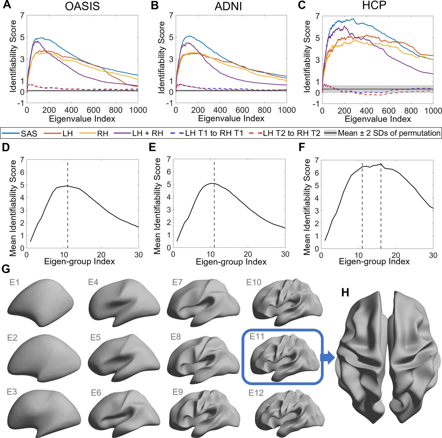
Identifiability of different shape descriptors at different spatial scales.
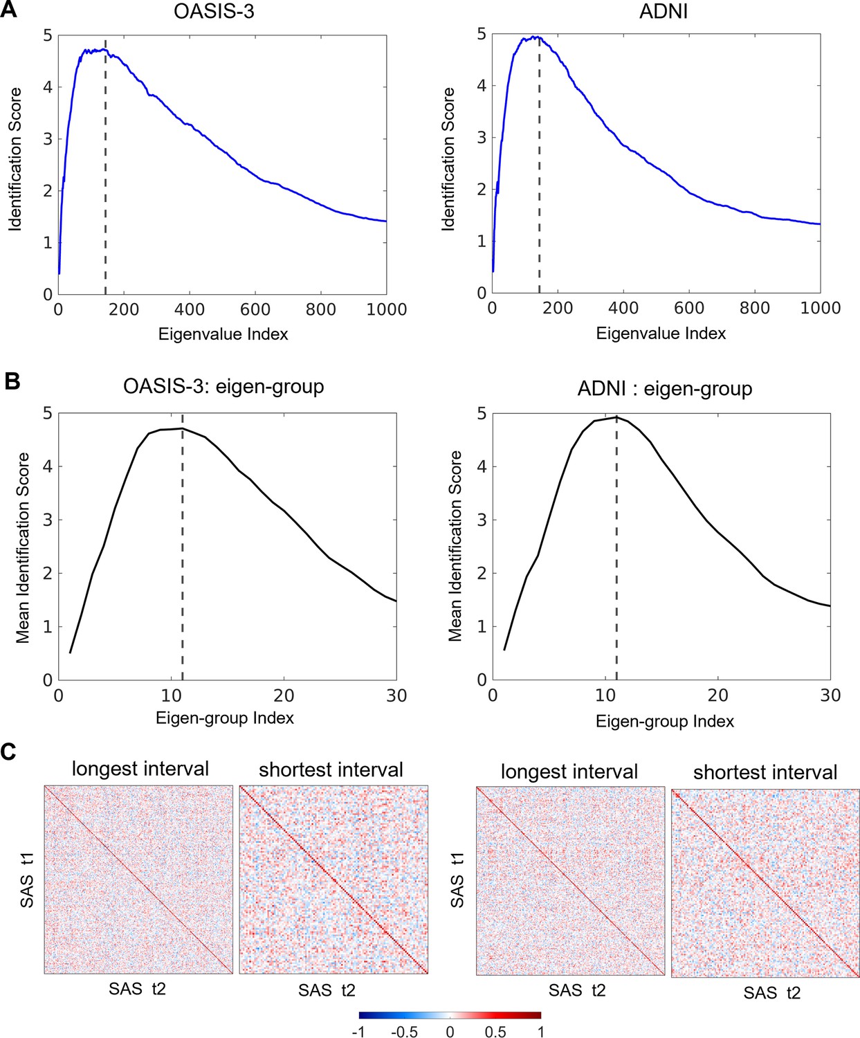
(A–C) Identifiability scores for shape features across eigenvalue indices. The identifiability scores of the shape asymmetry signature (SAS) are generally higher than the scores for shape descriptors of individual hemispheres or scores obtained when concatenating both hemispheres across three datasets (OASIS-3: n = 233; ADNI: n = 208; HCP test–retest: n = 45). The SAS scores are also much higher than the scores obtained by randomly shuffling the order of the subjects at time 2 (shaded area represents mean ± 2 SDs). (D–F) The cumulative mean identifiability scores for each eigenvalue group, derived from correspondence with spherical harmonics (Robinson et al., 2016). The peak mean identifiability occurs at the 11th eigenvalue group for the OASIS-3 (D) and ADNI data (E), representing the first 144 eigenvalues. The curve of the mean identifiability score for the HCP test–retest data (F) flattens after the 11th group and peaks at the 16th group. (G) Cortical surfaces reconstructed at different spatial scales, starting with only the first eigen-group (E1) and incrementally adding more groups to a maximum of the first 12 eigen-groups (E12). (H) Overhead view of the spatial scale corresponding to the eigen-group at which identifiability is maximal in the OASIS-3 and ADNI datasets (i.e., the first 11 eigen-groups, corresponding to the first 144 eigenvalues).
Figure 2—figure supplement 1
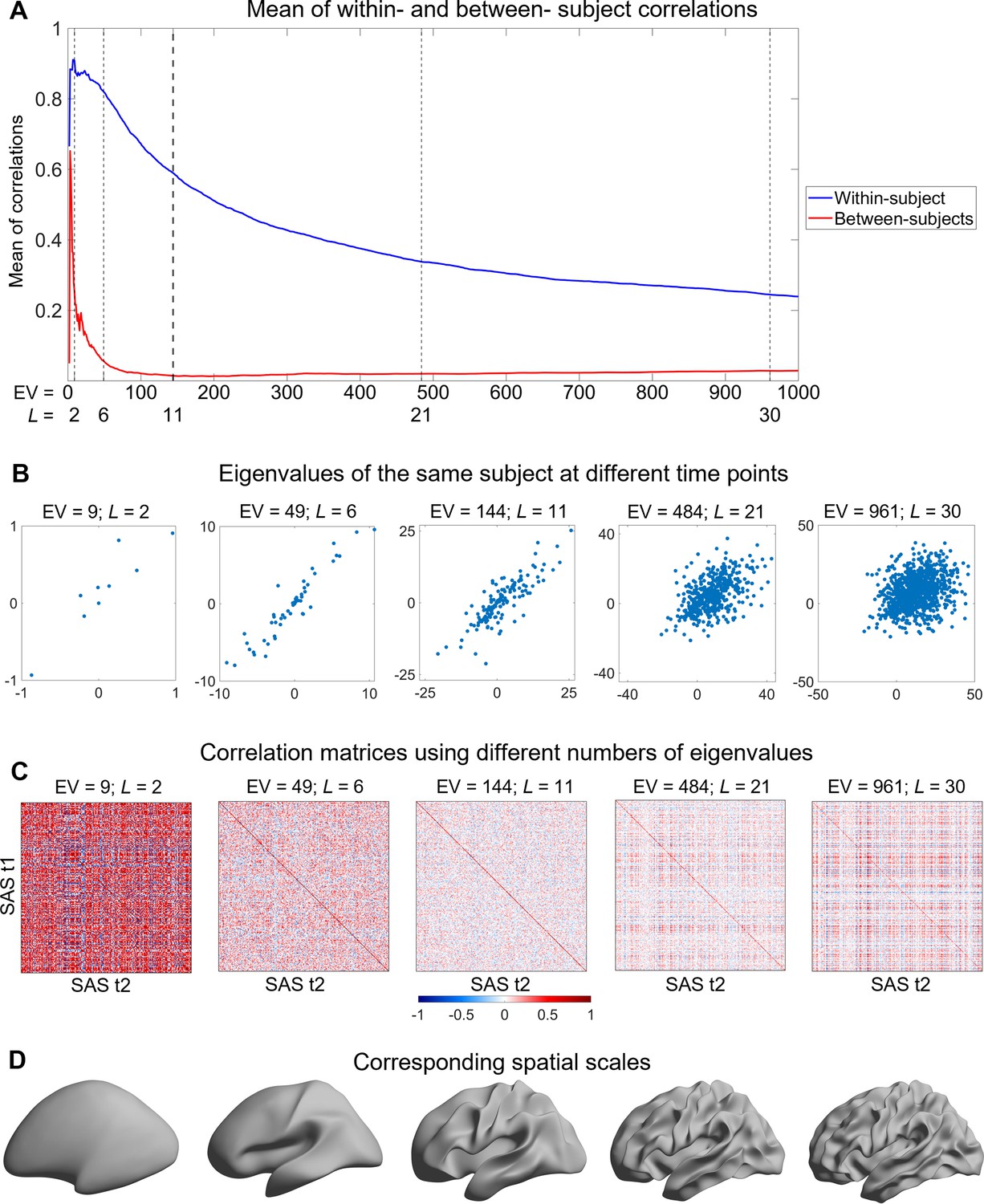
Understanding the identifiability score.
Here, we use the shape asymmetry signatures from the OASIS-3 subjects (n = 233) as an example. (A) The mean of both within- and between-subject correlations decrease at finer scales, but the between-subject correlations are lower and decline faster than the within-subject correlations. (B) The same subject at time 1 (t1) and time 2 (t2) with different numbers of eigenvalues. (C) Pearson correlation matrices using different numbers of eigenvalues. The diagonal elements are the within-subject correlations, and the off-diagonal elements are the between-subject correlations. Both within- and between-subject correlations are high from the very coarse scales (e.g., nine eigenvalues in panel C); both correlations are low if fine scales are involved (e.g., 961 eigenvalues in panel C). The number of eigenvalues with peak identifiability score (144 eigenvalues; L = 11) maximizes the difference between the between-subject and within-subject correlations. (D) Cortical surfaces reconstructed at spatial scales correspond to the eigen-groups in panel (C).
Figure 2—figure supplement 2
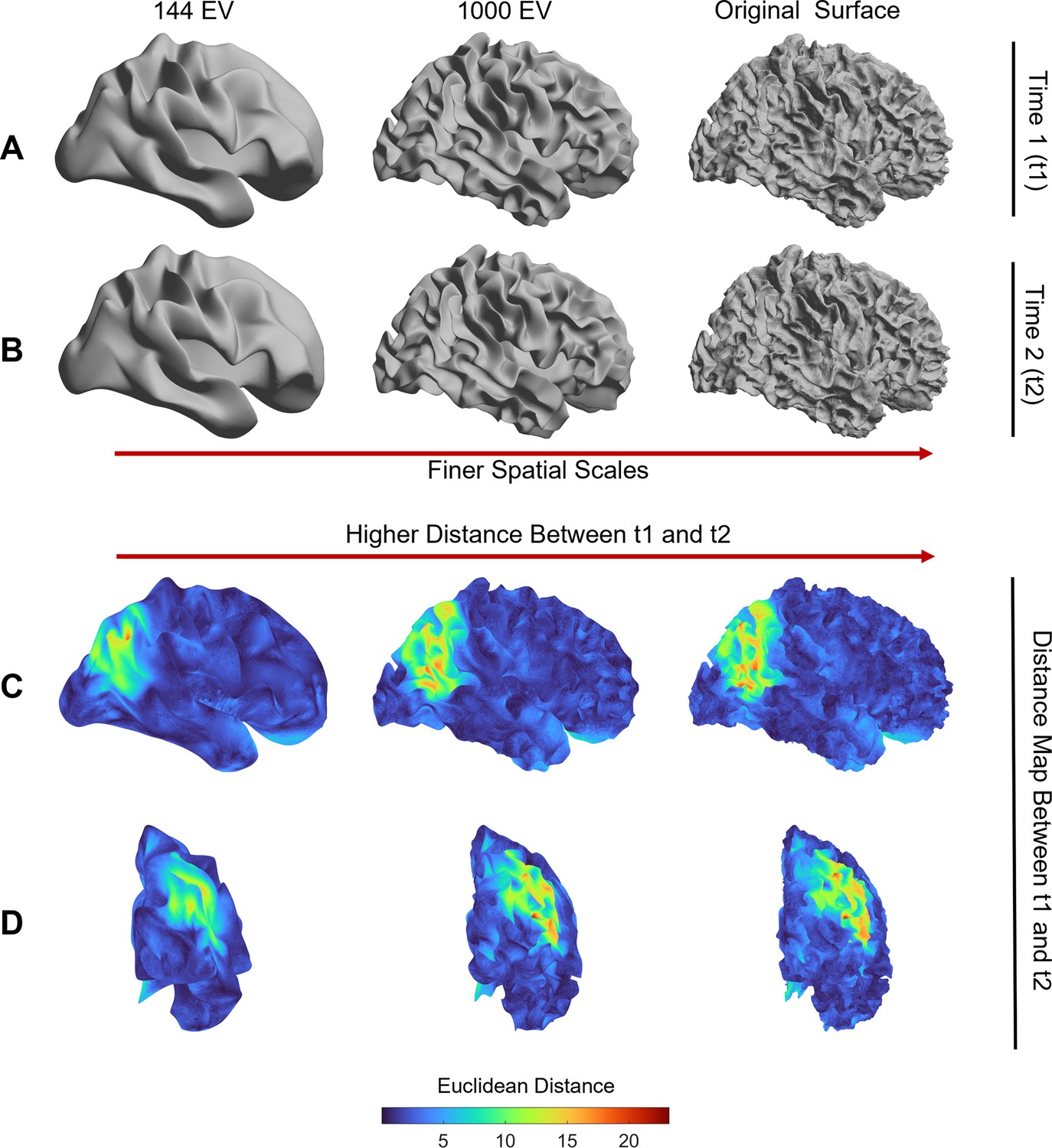
Inter-session variability in cortical shape is higher at more fine-grained spatial scales.
Panels (A) and (B) show the white surface of one participant from the OASIS-3 dataset reconstructed at three spatial scales (i.e., using 144 eigenmodes, 1000 eigenmodes, and the full cortical surface) for time 1 and time 2 sessions, respectively. Panels (C) and (D) map the Euclidean distance of mesh vertices between time 1 and time 2 at each spatial scale. The inter-session distances increase at finer scales (i.e., the original surface at the right panel). The images are registered on the fsaverage template.
Figure 2—figure supplement 3
Subject identifiability scores recalculated for data from MRI sessions with the longest inter-sessional interval.
The optimal spatial scales determined by eigen-groups are identical to the initial analysis using the shortest inter-sessional interval. (A) The peak subject identifiability score occurs at the combination of the first 136 and 139 eigenvalues in the OASIS-3 (n = 115) and ADNI (n = 135) data, respectively. (B) The peak mean subject identifiability score occurs at the first 11th eigen-groups, representing the first 144 eigenvalues, in both the OASIS-3 and ADNI data. (C) Pearson correlation matrices calculated using the first 144 eigenvalues for the OASIS-3 and ADNI data by using both the shortest (OASIS-3: n = 233; ADNI: n = 208) and longest inter-sessional intervals.
Figure 3 with 1 supplement

Cortical shape asymmetries are more identifiable than size-related descriptors or functional connectivity.
(A) Identifiability scores for the shape asymmetry signature (SAS) are higher than those obtained for asymmetries based on cortical surface area (identifiability score = 0.81), volume (identifiability score = 0.66), and thickness (identifiability score = 0.33) for the OASIS-3 dataset (n = 232; see ‘Materials and methods’). (B) Matrices of the Pearson correlation coefficients for SAS and size-based morphological asymmetries from MRI scans taken at different time points (t1 and t2) of the OASIS-3 subjects. (C) SAS identifiability is higher than the identifiability based on functional connectivity, assessed with parcellations at different resolution scales in the HCP test–retest dataset (n = 44). (D) Matrix of the Pearson correlation coefficients for SAS of the HCP test-retest subjects. (E) Four resolution scales of parcellations used in the functional connectivity analysis (shown on an inflated fsaverage surface in FreeSurfer). (F) Matrices of the Pearson correlation coefficients for functional connectivity using the Schaefer 100 (identifiability score = 1.57), HCP-MMP1 (identifiability score = 2.06), Schaefer 300 (identifiability score = 2.11), and Schaefer 900 (identifiability score = 2.69) parcellations.
Figure 3—figure supplement 1
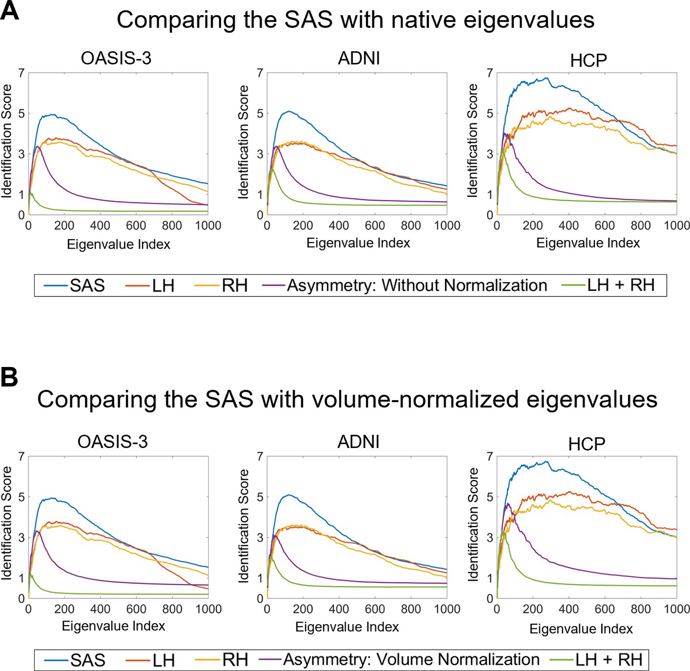
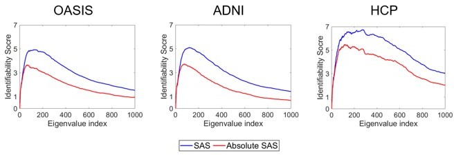
Comparing identifiability scores between the shape asymmetry signature (SAS) with either native eigenvalues or volume-normalized eigenvalues.
The identifiability scores calculated from the surface area normalized SAS are generally higher than the scores calculated using native eigenvalues and eigenvalues with volume normalization (but without surface area normalization) for individual hemispheres, the combination of both hemispheres, and asymmetry across three datasets (OASIS-3: n = 233; ADNI: n = 208; HCP: n = 45). (A) identifiability scores calculated from native eigenvalues (except the blue lines, which are the SAS); (B) identifiability scores calculated from eigenvalues with volume normalization (except the blue lines, which are the SAS).
Figure 4
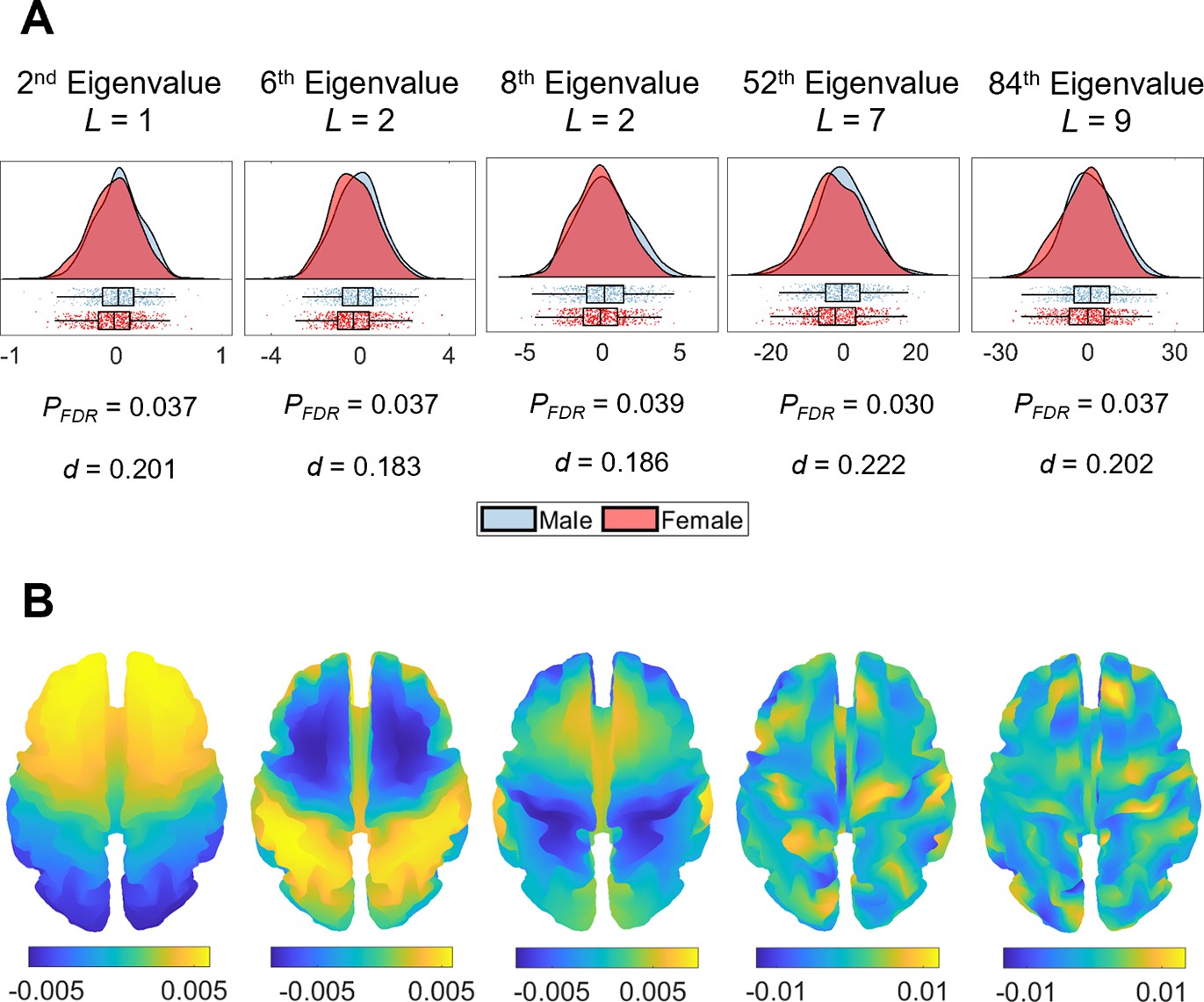
Sex differences in eigenvalue asymmetries.
(A) Smoothed distributions and boxplots with mean and interquartile range (Allen et al., 2019) of the eigenvalues among males (n = 504) and females (n = 602). Under these five spatial scales, female brains show a greater rightward asymmetry than males. The p-values are false discovery rate (FDR)-corrected values of the correlation between sex and shape asymmetry signature (SAS), obtained via a general linear model (GLM). The d values are effect sizes (Cohen’s d). L denotes eigen-group. (B) The corresponding eigenfunction of each eigenvalue in panel (A) that shows the gradients of spatial variation on a population-based template.
Figure 5
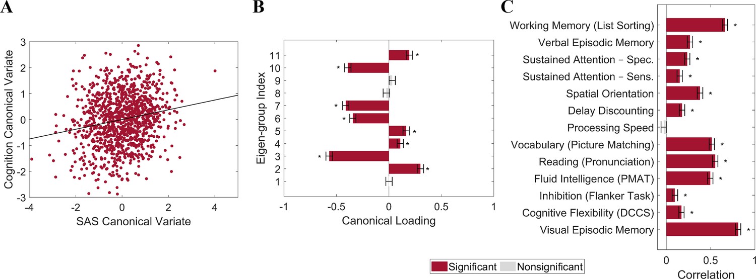
Individual differences in cortical shape asymmetry correlate with general cognitive ability.
(A) Scatterplot of the association between the cognitive and shape asymmetry signature (SAS) canonical variates with the corresponding least-squares regression line in black. (B) Canonical variate loadings of each eigen-group. (C) Correlations between the original cognitive measures and the cognitive canonical variate. Error bars show ±2 bootstrapped standard errors (SE). Asterisks denote bootstrapped PFDR < 0.05. The data in this figure are from the HCP dataset (n = 1106).
Figure 6 with 2 supplements
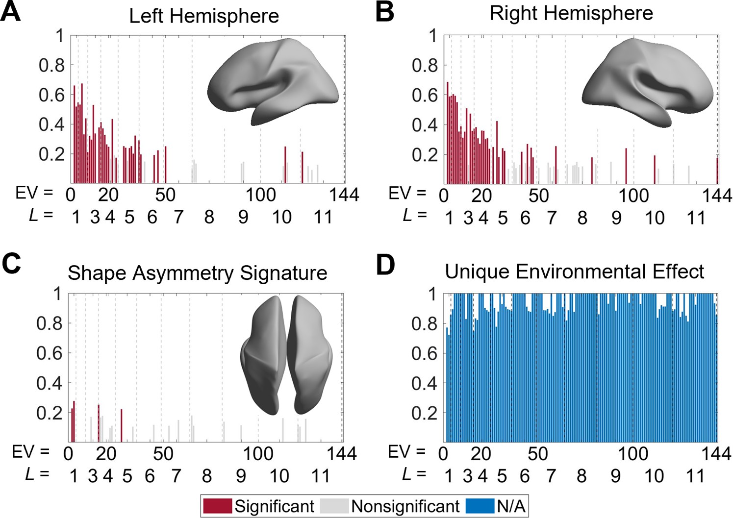
Heritability of cortical shape.
(A, B) Heritability of the eigenvalues of the left (A) and right (B) hemispheres. The insets show the corresponding spatial scales by reconstructing the surfaces using the first six eigen-groups. (C) Heritability of the shape asymmetry signature (SAS). The inset shows the corresponding spatial scale with some level of genetic influence, obtained by reconstructing the surface using the first five eigen-groups. (D) Unique environmental influences to the SAS at each eigenvalue. Statistical significance is evaluated after false discovery rate (FDR) correction. Note that significance is not estimated for unique environmental effects as this represents the reference model against which other genetically informed models are compared. We use 79 same-sex dizygotic (DZ) twin pairs, 138 monozygotic (MZ) twin pairs, and 160 of their non-twin siblings.
Figure 6—figure supplement 1
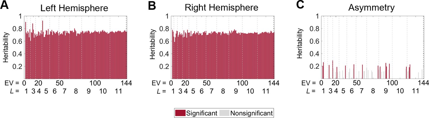
Heritability of cortical shape with volume normalization but without normalizing the surface area.
(A, B) The heritability of the eigenvalues from the left (A) and right (B) hemispheres are uniformly high across all eigenvalues, and the scale-specific effects are eliminated. The heritability estimates are very close to the heritability of the mean of the cortical volumes across all regions of the MMP1 atlas ( for the left hemisphere and for the right hemisphere). This result indicates that even normalizing the cortical volume, the heritability estimates are still highly influenced by the volume rather than purely by the shape. (C) Heritability estimates of the asymmetry are lower than that of the individual hemispheres but still have no scale effects. Statistical significance is evaluated after false discovery rate (FDR) correction. We use 79 same-sex dizygotic twin pairs, 138 monozygotic twin pairs, and 160 of their non-twin siblings.
Figure 6—figure supplement 2
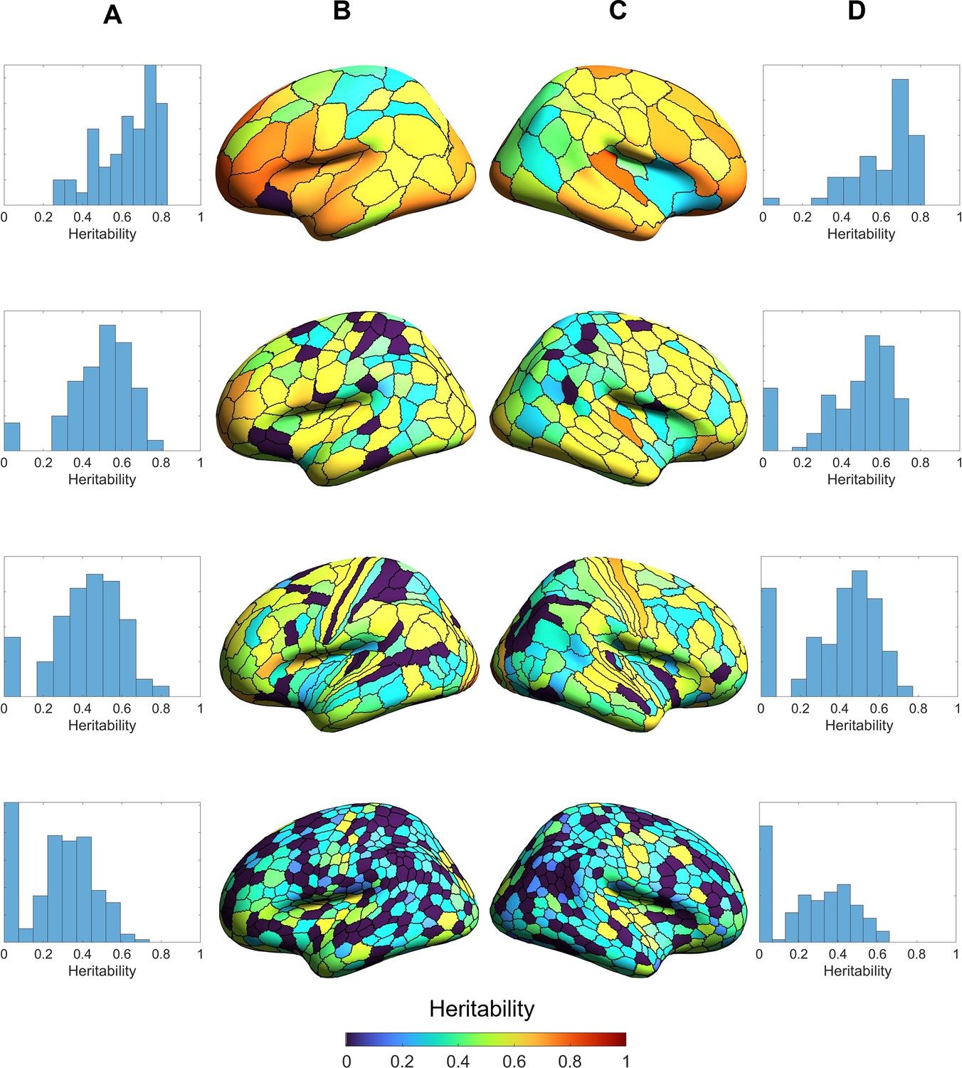
Heritability estimates of regional volumes of individual hemispheres across four parcellation resolutions: Schaefer 100, Schaefer 300, HCP-MMP1, and Schaefer 900 (top to bottom panels).
Generally, heritability estimates are higher at coarser (upper panels) than finer parcellation resolutions (lower panels). (A) and (D) are the distributions of the regional heritability estimates of the left (A) and right (D) hemispheres. (B) and (C) are heritability estimates of each region of the left (B) and right (C) hemispheres.
Figure 7

Eigenvalue spectra with and without normalization.
(A) Native eigenvalue spectra. (B) Eigenvalue spectra with volume normalization. (C) Eigenvalue spectra with surface area normalization. All of these results are from the left white surfaces of 233 subjects from the OASIS- 3 data. Each line represents a subject. The slopes of the spectra in (A) and (B) differ among subjects, whereas those in (C) are almost identical.
Author response image 1
Additional files
-
Supplementary file 1
Wavelength and eigenvalue indices of each eigen-group.
- https://cdn.elifesciences.org/articles/75056/elife-75056-supp1-v3.docx
-
Transparent reporting form
- https://cdn.elifesciences.org/articles/75056/elife-75056-transrepform1-v3.pdf
Download links
A two-part list of links to download the article, or parts of the article, in various formats.
Downloads (link to download the article as PDF)
Open citations (links to open the citations from this article in various online reference manager services)
Cite this article (links to download the citations from this article in formats compatible with various reference manager tools)
The individuality of shape asymmetries of the human cerebral cortex
eLife 11:e75056.
https://doi.org/10.7554/eLife.75056


