Three-dimensional structure of kinetochore-fibers in human mitotic spindles
Figures

Models of k-fiber organization in mammalian mitosis.
(A) Direct connection with KMTs (red lines) spanning the distance between the kinetochore and the spindle pole. Chromosomes are shown in blue with kinetochores in red. The mother (m) and the daughter centriole (d) of the spindle pole are indicated. All KMTs are assumed to have similar lengths. (B) Indirect connection showing KMTs linking the kinetochore and the spindle pole by association with non-KMTs (yellow lines). K-fibers in this model are composed of KMTs with different lengths, and none of the KMTs is directly associated with the spindle pole. (C) Semi-direct connection showing KMTs of different lengths. Some KMTs are directly associated with the spindle pole, while others are not. In this model, KMTs show a difference in length.
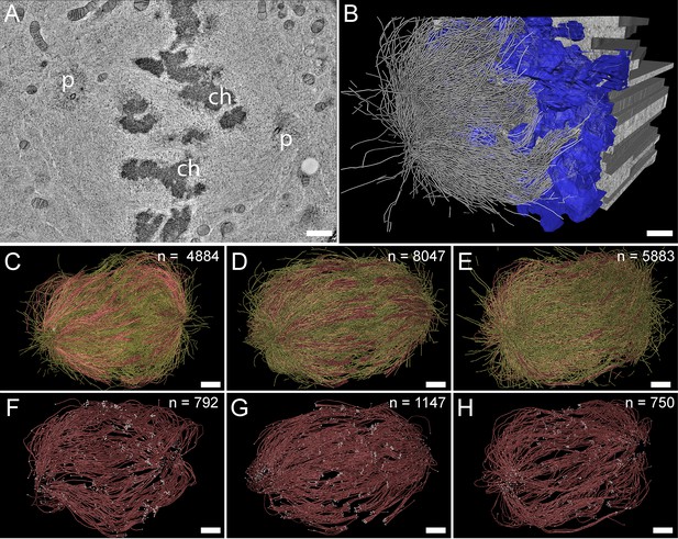
Three-dimensional reconstruction of metaphase spindles by large-scale electron tomography.
(A) Tomographic slice showing a HeLa cell (spindle #1) in metaphase. The chromosomes (ch) and the spindle poles (p) are indicated. (B) Three-dimensional reconstruction of the same spindle as shown in A. The stacking of the serial tomograms used to generate a three-dimensional model of the spindle with the MTs (white lines) is visualized. The segmented chromosomes are shown in blue. (C) Three-dimensional model of the spindle as shown in A. The total number of all MTs is given in the upper right corner. The non-KMTs (yellow lines) and KMTs (red lines) are shown. (D) Full 3D model of metaphase spindle #2. (E) Full 3D model of metaphase spindle #3. (F) Extraction of KMTs from the 3D reconstruction as shown in C. The number of KMTs is given in the upper right corner. KMT plus and minus ends are shown by white spheres. (G) KMTs extracted from spindle #2. (H) KMTs extracted from spindle #3. Scale bars, 1 µm.
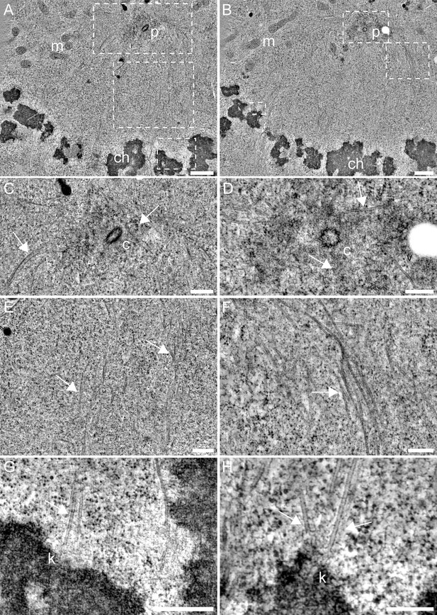
Illustration of metaphase in HeLa cells.
(A–B) Tomographic slices through spindle #3 illustrating the morphology of HeLa cells. Spindle poles (p) with a centriole, chromosomes (ch), and mitochondria (m) are indicated. The boxed regions (from top to bottom) show a spindle pole, MTs in between a spindle pole and the chromosomes, and a kinetochore region with attached KMTs. Scale bars, 500 nm. (C–D) Tomographic slices showing the centrioles (c) and MTs (white arrows) at higher magnification (corresponds to the top boxes in A-B). Scale bars, 250 nm. (E–F) Region of the cell between a spindle pole and the chromosomes. MTs (white arrows) are marked (corresponds to the mid boxes in A-B). Scale bars, 250 nm. (G–H) Kinetochores (k) with associated KMTs (marked by arrows) are shown (corresponds to the bottom boxes in A-B). Scale bars, 250 nm.
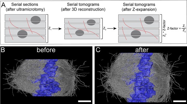
Correction of sample collapse caused during data acquisition by electron tomography.
(A) Schematic illustration of correction for a sample collapse in Z. Left panel shows a stack of semi-thick sections after ultramicrotomy (total height, Z1). The mid panel illustrates a sample collapse as obvious after computational stacking of the serial tomograms (total height, Z2). Right panel, calculation of the Z-factor (Z1/Z2) and correction of the collapse by application of the Z-factor (Z2*Z-factor). (B) Side view (Y/Z orientation) of the 3D reconstructed spindle #1 before Z-expansion. (C) Side view of the same spindle after Z-expansion. Scale bars, 1 µm.
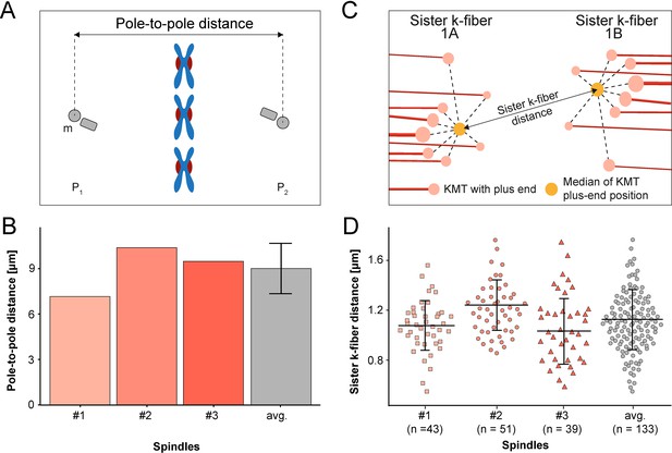
Analysis of pole-to-pole and sister k-fiber-to-sister k-fiber distances.
(A) Schematic illustration of the pole-to-pole distance. The 3D distance between the mother centrioles (m, marked in gray) of the two opposing spindle poles (P1 and P2) is measured. Chromosomes (blue) and kinetochores (red) are also shown. (B) Bar plot showing the pole-to-pole distance for each data and the average of all data sets (error bars are mean ±STD, n=3). (C) Schematic illustration of the distance between the KMT plus ends of sister k-fibers (called 1 A and 1B). The KMTs (red lines) with their plus ends (light red circles) are indicated. The median position (yellow circle) of all KMT plus ends was calculated for each kinetochore pair. (D) Graph showing the average 3D distance between sister k-fibers for each data set and for all data sets (error bars are mean ±STD). The number of measurements per dataset is indicated.
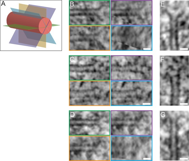
Morphology of KMT plus ends.
(A) Schematic illustration of a KMT (red tube) with different viewing planes (colored in green, blue, orange, and purple). (B–D) Tomographic slices of KMT plus ends visualized at different viewing planes (as illustrated in A). Scale bars, 25 nm. (E–G) Average intensity Z projections of the KMT plus ends as shown in B-D. The KMTs show flared open plus ends. Scale bars, 25 nm.
Generation of a 3D model from joined serial electron tomograms displaying spindle #1.
Series of stitched tomograms and corresponding 3D model of spindle #1. The stacking of serial tomograms to increase the tomographic volume is illustrated. MTs are shown as white lines, and chromosomes are illustrated in blue. This video corresponds to Figure 2C. Scale bar, 1 µm.
Generation of a 3D model from joined serial electron tomograms displaying spindle #2.
Series of stitched tomograms and corresponding 3D model of spindle #2. The stacking of serial tomograms to increase the tomographic volume is illustrated. MTs are shown as white lines, and chromosomes are illustrated in blue. This video corresponds to Figure 2D. Scale bar, 2 µm.
Generation of a 3D model from joined serial electron tomograms displaying spindle #3.
Series of stitched tomograms and corresponding 3D model of spindle #3. The stacking of serial tomograms to increase the tomographic volume is illustrated. MTs are shown as white lines, and chromosomes are illustrated in blue. This video corresponds to Figure 2E. Scale bar, 2 µm.
Organization of KMTs in spindle #1.
Three-dimensional model of spindle #1. Non-KMTs are shown in yellow, KMTs in red. Chromosomes are illustrated in blue and centrioles in gray. This video corresponds to Figure 2F. Scale bar, 1 µm.
Organization of KMTs in spindle #2.
Three-dimensional model of spindle #2. Non-KMTs are shown in yellow, KMTs in red. Chromosomes are illustrated in blue and centrioles in gray. This video corresponds to Figure 2G. Scale bar, 1.5 µm.
Organization of KMTs in spindle #3.
Three-dimensional model of spindle #3. Non-KMTs are shown in yellow, KMTs in red. Chromosomes are illustrated in blue and centrioles in gray. This video corresponds to Figure 2H. Scale bar, 1.5 µm.
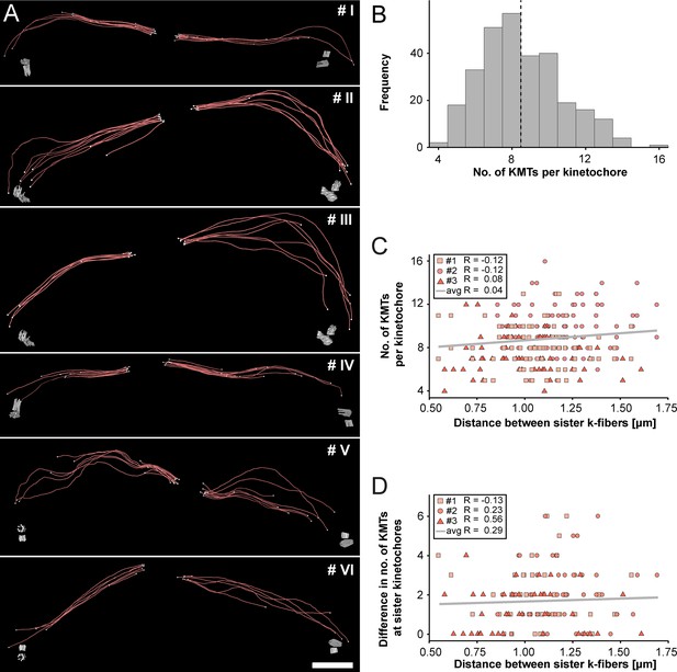
Morphology of k-fibers and number of KMTs associated per kinetochore.
(A) Examples of individual sister k-fibers extracted from the full 3D reconstruction of metaphase spindle #1. The numbering of these examples (corresponding to the supplementary videos) is given in the upper right corners. KMTs are shown as red lines. The ends of the KMTs are indicated by white spheres, centrioles are shown as cylinders (gray). Scale bar for all examples, 1.5 µm. (B) Histogram showing the frequency of detected KMTs per kinetochore. This plot includes data from all three spindle reconstructions. The dashed line (black) indicates the average number of KMTs per kinetochore (n=292). (C) Graph showing the number of KMTs associated per kinetochore plotted against the distance between sister k-fibers (n=292). The Pearson’s correlation coefficient for each data set and the average coefficient for all data sets are given. (D) Graph showing the difference (delta) in the number of KMTs associated with the respective sister kinetochores plotted against the distance between the kinetochore-proximal ends of k-fiber pairs (n=292). The Pearson’s correlation coefficient for each data set and the average coefficient for all data sets are given.
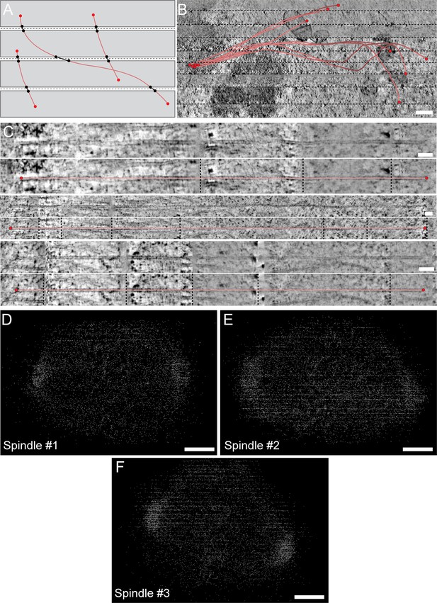
MT segmentation and stitching across consecutive serial sections.
(A) Schematic illustration of MT segmentation across stacked consecutive serial sections. Each section is represented as a gray area. MTs are shown as red lines and their ends as red circles. ‘Artificial ends’ at section borders that need to be stitched are labeled by black circles. The horizontal dashed lines (black) indicate the seams between the sections. (B) Stacked serial tomograms showing a selected k-fiber that has been followed over several serial sections. The KMTs are indicated as red lines and the ends are marked by red circles. The dashed lines (black) indicate the seam regions. Scale bar, 250 nm. (C) Longitudinal views of KMTs of the same k-fiber as shown in B. Borders of the serial sections are indicated by vertical dashed lines. The top rows of each reconstruction show selected traced KMTs. The bottom rows show the same KMTs with overlays to indicate the length (red line) and the ends (red circles) of each KMT. Scale bars, 50 nm. (D) Y/Z view of the 3D model of spindle #1 showing MT tracings at section borders. Scale bar, 500 nm. (E) Y/Z view of spindle #2. Scale bar, 600 nm. (F) Y/Z view of spindle #3. Scale bar, 500 nm.
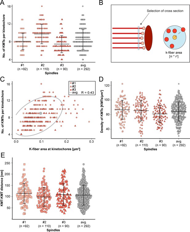
Correlation of k-fiber circumference and number of attached KMTs.
(A) Graph showing the number of KMTs per kinetochore for each data set and the average number for all data sets (error bars are mean ±STD). (B) Schematic illustration of the indirect measurement of the k-fiber area. MTs (red lines) with their ends (circles in light red) and the kinetochore (ellipsoid in dark red) are shown (left). The measurement of the cross-section of a k-fiber in the vicinity of the KMT ends is indicated by a blue bar. The k-fiber area (right) is given by a blue circle enclosing all KMTs (center of the circle in orange). (C) Graph showing the number of KMTs per kinetochore for all reconstructed spindles plotted against the area of k-fibers at the kinetochore (n=292). The ellipse (gray) indicates a 95% confidence interval for all data and the central dot (gray) indicates the average kinetochore area. (D) Graph showing the density of KMTs at the kinetochore for each 3D reconstruction and for all data sets (error bars are mean ±STD). (E) Plot showing the average KMT-to-KMT distance at the kinetochore for all data sets (error bars are mean ±STD). The average for all data sets is also given.
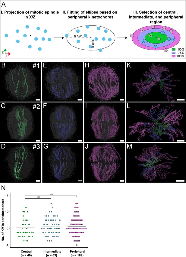
Positioning of k-fibers in the mitotic spindle.
(A) Schematic illustration of the k-fiber positions on the X/Z projection of the metaphase plate. Kinetochores are indicated as blue circles. The fitted ellipse (center marked by a black dot) including all kinetochores is characterized by the semi-major (a-) and the semi-minor (b-) axis. The ellipse is divided into three areas representing the percentage of occupancy on the ellipse (0–50%, central kinetochores, green; 50–75%, intermediate kinetochores, blue; and 75–100%, peripheral kinetochores, purple). (B–D) Perspective views of the reconstructed spindles with selected central k-fibers (green). The number of each spindle is indicated (upper right corners). (E–G) Perspective views with selected intermediate k-fibers (blue). (H–J) Perspective views with selected peripheral k-fibers (purple). (K–M) Cross-section views of the spindles with all k-fiber classes. (N) Plot showing the number of KMTs per kinetochore according to the three positional regions in the mitotic spindle for all data sets. The mean of the KMT number is indicated (black horizontal lines). A Student’s t-test was applied for statistical analysis. Scale bars, 1 µm.
3D reconstruction of a single k-fiber pair.
Three-dimensional model of selected sister k-fibers in spindle #1. The KMTs are shown as red lines, KMT ends as white spheres and the centrioles as gray cylinders. This video corresponds to Figure 3A (k-fiber pair # I). Scale bar, 1 µm.
3D reconstruction of a single k-fiber pair.
Three-dimensional model of selected sister k-fibers in spindle #1. The KMTs are shown as red lines, KMT ends as white spheres and the centrioles as gray cylinders. This video corresponds to Figure 3A (k-fiber pair # II). Scale bar, 1 µm.
3D reconstruction of a single k-fiber pair.
Three-dimensional model of selected sister k-fibers in spindle #1. The KMTs are shown as red lines, KMT ends as white spheres and the centrioles as gray cylinders. This video corresponds to Figure 3A (k-fiber pair # III). Scale bar, 1 µm.
3D reconstruction of a single k-fiber pair.
Three-dimensional model of selected sister k-fibers in spindle #1. The KMTs are shown as red lines, KMT ends as white spheres and the centrioles as gray cylinders. This video corresponds to Figure 3A (k-fiber pair # IV). Scale bar, 1 µm.
3D reconstruction of a single k-fiber pair.
Three-dimensional model of selected sister k-fibers in spindle #1. The KMTs are shown as red lines, KMT ends as white spheres and the centrioles as gray cylinders. This video corresponds to Figure 3A (k-fiber pair # V). Scale bar, 1 µm.
3D reconstruction of a single k-fiber pair.
Three-dimensional model of selected sister k-fibers in spindle #1. The KMTs are shown as red lines, KMT ends as white spheres and the centrioles as gray cylinders. This video corresponds to Figure 3A (k-fiber pair # VI). Scale bar, 1 µm.

Analysis of MT length distribution.
(A) Histogram showing the length distribution of KMTs from all data sets (n=2579). The dashed line indicates the average length of KMTs. (B) Histogram showing the length distribution of non-KMTs (n=14458). The dashed line indicates the average length of non-KMTs.
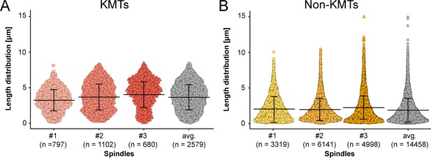
Length distribution of KMTs and non-KMTs.
(A) Beeswarm plot showing the length distribution of KMTs in the individual data sets. The average of all data sets is also given (error bars are mean ±STD). (B) Beeswarm plot showing the length distribution of non-KMTs in the individual data sets The average of all data sets is also given (error bars are mean ±STD).
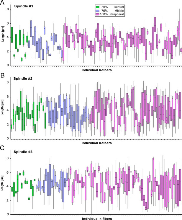
KMT length distribution based on the k-fiber position in the spindle.
(A) Box plot showing the length distribution of KMTs in individual k-fibers as observed in spindle #1 (n=98). The k-fibers are displayed and color-coded according to their position within the spindle (insert). For each k-fiber, error bars are mean ±STD. (B) KMT length distribution in spindle #2 (n=110). (C) KMT length distribution in spindle #3 (n=90).
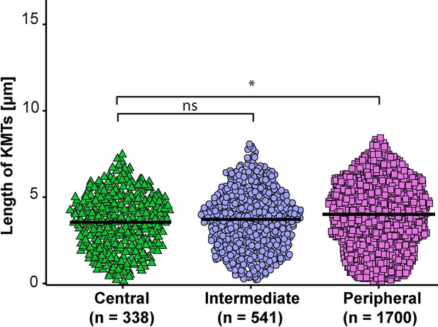
KMT length distribution based on the position of individual k-fibers within the spindle.
Beeswarm plot showing the length distribution of KMTs and the average of all data sets based on the k-fiber position in the spindle. The plots show the mean indicated by black horizontal bars. The statistical significance (p<0.001) was calculated with a Student’s t-test.
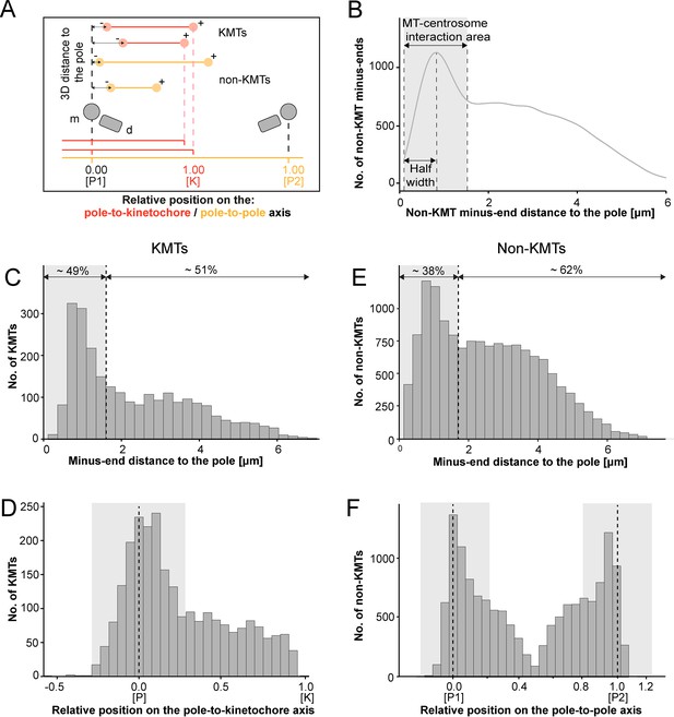
Analysis of MT minus ends.
(A) Measurement of MT minus-end positioning. A KMT (red line) with its ends (red circles) and a non-KMT (yellow line) with its ends (yellow circles) are shown. The distance of both the KMT and the non-KMT minus ends to the center of the mother centriole was calculated. The relative position of the KMT minus ends along the pole-to-kinetochore axis and the non-KMT minus ends along the pole-to-pole axis was also determined (P1, pole 1; P2, pole 2; K, kinetochore). (B) Determination of the MT-centrosome interaction area. Graph showing the number of non-KMT minus ends plotted against their distance to the pole (i.e. to the center of the mother centriole). The determined area of the interaction of non-KMTs with the centrosome and the half-width of this area is indicated in gray. The border of the MT-centrosome interaction area (right dashed line) was determined by identifying twice the half-width of the distribution peak of the minus-end distances. (C) Histogram showing the distribution of the KMT minus-end distances to the center of the mother centriole (n=2579). The MT-centrosome interaction area as defined in B is indicated by a gray area (dashed line shows the border of this area). (D) Histogram showing the relative position of the KMT minus ends on the pole-to-kinetochore axis (n=2579). The position of the spindle pole (p = 0, dashed line) and the kinetochore (K = 1) is indicated. The approximated MT-centrosome interaction area is indicated in gray. (E) Histogram showing the distribution of the non-KMT minus-end distances to the center of the mother centriole (n=14458). The MT-centrosome interaction area is indicated in gray. (F) Plot showing the relative position of the non-KMT minus ends on the pole-to-pole axis (n=14458). The position of the spindle poles (P1 = 0, P2 = 1). The approximated MT-centrosome interaction area is shown in gray.
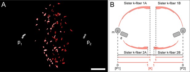
Normalization of minus-end positioning on the pole-to-kinetochore axis.
(A) Three-dimensional model of the kinetochores visualized in spindle #1. For each kinetochore pair, each kinetochore is assigned to the closest spindle pole (p1, left pole, kinetochores in light red; p2, right pole, kinetochores in dark red). (B) Schematic drawing illustrating the normalization of KMT minus-end positioning (spindle pole positions, P1 and P2 = 0; kinetochore position = 1). End positioning is then determined between positions 0 and 1 for each k-fiber.
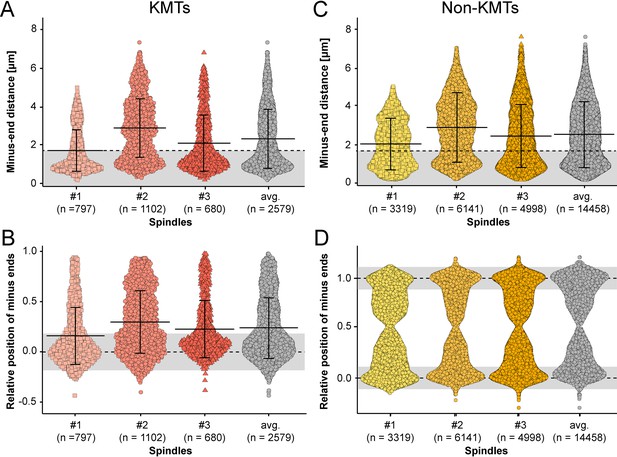
Minus-end distribution of KMTs and non-KMTs.
(A) Beeswarm plot showing the distribution of KMT minus-end distances to the center of the mother centrioles. The MT-centrosome interaction area is indicated in gray (error bars are mean ±STD). (B) Plot showing the distribution of relative positioning of the KMT minus ends on the pole-to-kinetochore axis (position of the spindle pole = 0; position of the kinetochore = 1; error bars are mean ±STD). (C) Distribution of the distances of the non-KMT minus ends to the center of the mother centriole (error bars are mean ±STD). (D) Distribution of relative positioning of the non-KMT minus ends on the pole-to-kinetochore axis. The approximated MT-centrosome interaction areas (in B and D) are shown in gray.
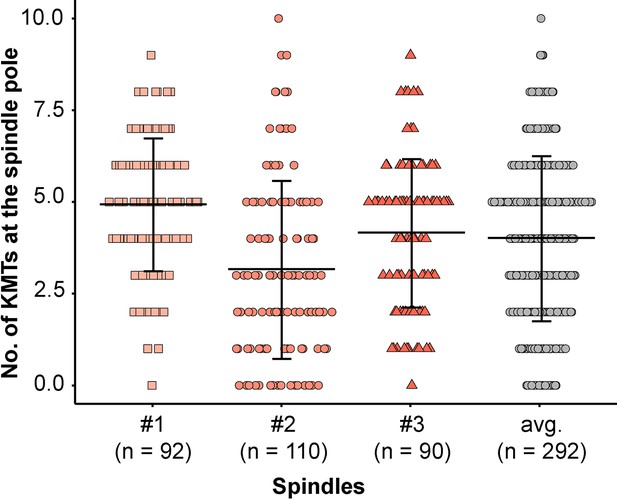
Analysis of KMT minus ends reaching the pole.
Plot showing the number of KMT minus ends per k-fiber detected within the MT-centrosome interaction area. The individual data sets and the average numbers for all data sets are given (error bars are mean ±STD).
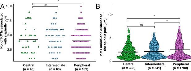
KMT minus-end distribution based on the k-fiber position in the spindle.
(A) Plot showing the number of KMTs in each k-fiber associated with the spindle poles for the three positional regions in the mitotic spindle for all data sets. The mean values are indicated. (B) Beeswarm plot showing the distance of KMT minus-ends to the center of the mother centrioles for all KMTs. The mean values are shown by black horizontal lines. The statistical significance (p<0.001) was calculated with a Student’s t-test.
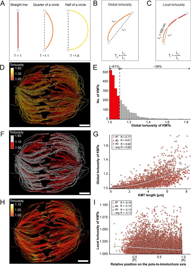
Global and local tortuosity of KMTs.
(A) Schematic illustration of tortuosity (T) as given for a straight line, a quarter of a circle, and a half of a circle. (B) Schematic illustration of global tortuosity (Tg) of KMTs given by the ratio of the spline length (Lx) to the 3D distance between the KMT ends illustrated by gray circles (Ly). (C) Schematic illustration of KMT local tortuosity (Tl) as given by division segments with a length of 500 nm. (D) Three-dimensional model of k-fibers (spindle #1) showing the global tortuosity of KMTs as indicated by color coding (top left corner). (E) Histogram showing the frequency of tortuosity for KMTs (n=2579). The Pearson’s correlation coefficient is given for each reconstructed spindle. The black dashed line indicates the average KMT tortuosity. The percentage ratio of ‘straight’ to ‘curved’ KMTs is also given. (F) Perspective view as shown in D. Straight KMTs (tortuosity of 1.0–1.1; red) and curved KMTs (tortuosity ≥1.1; white) are highlighted. (G) Correlation of global tortuosity and length of KMTs (n=2579). The Pearson’s correlation coefficient is given for each reconstructed spindle. The gray line indicates the local regression calculated by the loess method. (H) Three-dimensional model of k-fibers (from spindle #1) showing the local tortuosity of KMTs as indicated by color-coding. (I) Correlation of the local tortuosity of KMTs with the relative position along the pole (P)-to-kinetochore (K) axis (n=2579). Scale bars, 1 µm.
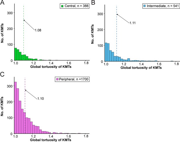
Global tortuosity of KMTs based on the k-fiber position in the spindle.
(A) Histogram showing the number of central KMTs plotted against the global tortuosity (n=338). (B) Histogram showing intermediate KMTs (n=541). (C) Histogram showing peripheral KMTs (n=1700). The mean global tortuosity of each k-fiber position is indicated by a dashed line.
Analysis of k-fiber global tortuosity in spindle #1.
Analysis of k-fiber global tortuosity in spindle #2.
Analysis of k-fiber global tortuosity in spindle #3.
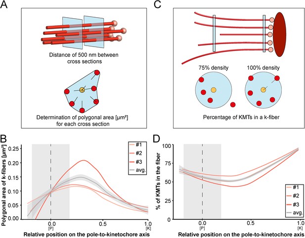
Shape of k-fibers.
(A) Schematic illustration of the analysis of polygonal areas as obtained from k-fiber cross-sections. KMTs are shown as lines (red), KMT ends as spheres (light red). Cross-sections of the given k-fiber are shown as blue squares (top). The median position of all KMTs in a cross-section is indicated as a yellow circle (bottom). (B) Distribution of the k-fiber polygonal area along with the relative position on the pole [P]-to-kinetochore [K] axis (n=292). (C) Schematic illustration of the k-fiber density analysis. For each k-fiber, a radius at the kinetochore was estimated by calculating a minimum circle enclosing all KMTs (top). The determined radius was then enlarged by factor 2 to account for k-fiber flexibility. Along with the k-fiber, the number of KMTs enclosed in the selected radius was then measured (bottom). (D) Distribution of the percentage of KMTs enclosed in the k-fiber along with the relative position along the pole [P]-to-kinetochore [K] axis (n=292). For each reconstructed spindle, data sets are presented as polynomial lines showing local regression calculated with the loess method. Average values with standard deviations are shown in gray. The approximated MT-centrosome interaction areas are shown in gray with the position of the poles indicated by dashed lines (B and D).
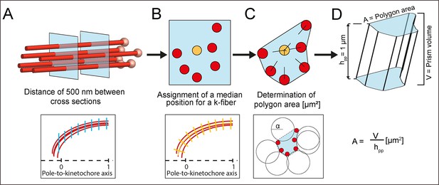
Schematic illustration of the analysis of k-fiber area and KMT density.
(A) Selection of cross-sections along a k-fiber (KMTs, red lines; KMT ends, light red spheres) every 500 nm (upper row - blue squares; lower row - blue lines). (B) Assignment of a median position (upper row - yellow circle; lower row, yellow line) for each cross-section and geometric correction of each cross-section based on the k-fiber’s curvature (lower row - yellow short lines). (C) Calculation of the polygonal area (upper row). The polygonal area was calculated using the alpha shape algorithm. For each cross-section, circles with a diameter defined by α (lower row - black lines) were fitted around the 2D projection of KMTs. The polygonal α-shape was created by drawing lines around KMTs that were at the junction of fitted circles (lower row - black dashed lines). (D) Calculation of the polygonal area from the created prism shape. For this, a polygonal area was duplicated and moved in Euclidean space by 1 μm in each dimension to create a prism shape. The polygonal area (A) is given by dividing the prism volume [μm3] by the prism height (hpp = 1 μm).
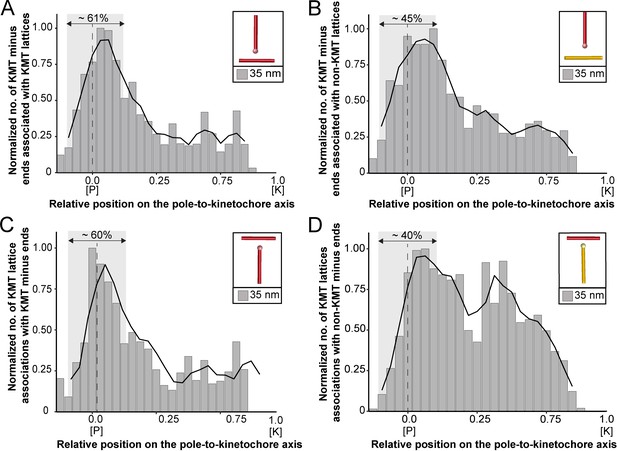
Association of KMTs with the MT network.
(A) Graph showing the number of KMT minus ends associated with KMT lattices within 35 nm of interaction (n=2579). Numbers of KMT minus ends are normalized by the density of surrounding MTs and plotted against the relative position on the pole-to-kinetochore axis (P, pole; K, kinetochore). The approximated MT-centrosome interaction area is shown in gray with the position of the pole indicated by a dashed line. The percentage of KMT associations located in the MT-centrosome interaction area is given. (B) Bar plot showing the normalized number of KMT minus ends associated with non-KMT lattices within 35 nm distance (n=2579). (C) Graph showing the number of KMT lattices associated with other KMT minus ends plotted along the relative position on the pole-to-kinetochore axis and normalized by the spindle density (n=2579). (D) Graph displaying the number of KMT lattices associated with non-KMT minus ends (n=2579). Moving averages with a period of 0.05 along the pole-to-kinetochore axis are shown as black lines.
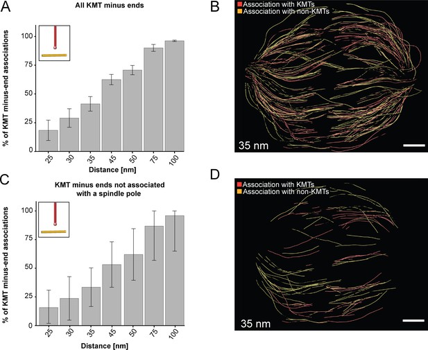
Association of KMT minus ends with other MT lattices.
(A) Bar plot showing the percentage of all KMT minus ends associated with a MT lattice depending on defined distances of interaction (25–100 nm; n=2579; error bars are mean ±STD). (B) Three-dimensional model showing the interaction pattern of all KMT minus ends associated with MTs. The distance of interaction is 35 nm (data obtained from spindle #1). KMT minus ends associated with other KMTs are labeled in red, KMT minus-endend association with non-KMTs is marked in yellow. (C) Bar plot showing the percentage of KMT minus ends not associated with the centrosome interaction area (error bars are mean ±STD; n=1558). The associations are shown for the defined distances of interaction. (D) Three-dimensional model of KMT minus ends associated with MT lattices but not attached to the pole (color coding of the associations as displayed in the B). Scale bars, 1 µm.
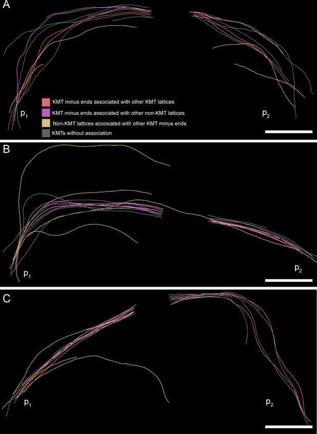
Association of KMT minus ends with KMT and non-KMT lattices at an interaction distance of 35 nm.
(A) Visualization of KMTs and non-KMTs obtained from the ASGA 3D-Viewer (https://cfci.shinyapps.io/ASGA_3DViewer/) showing a k-fiber pair from spindle #1 (ASGA k-fiber ID: pole1_08). This 3D model illustrates the association of KMT minus ends with MT lattices. The types of association are shown by color-coding (top image). The distance of interaction is 35 nm. The approximated position of the spindle poles (p1, p2) is indicated. (B) Model of k-fiber pair with ID: pole1_20. (C) Model of k-fiber pair with ID: pole1_23. Scale bars, 1 µm.
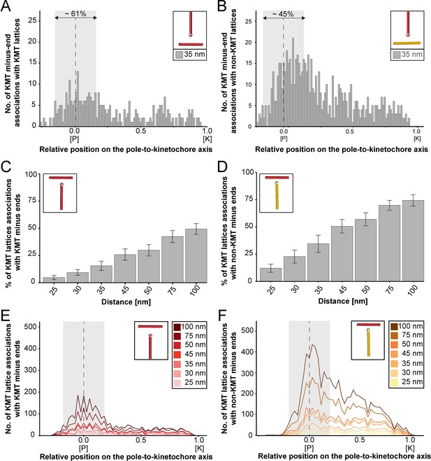
Association of KMTs with other MTs.
(A) Graph showing the number of KMT minus ends associated with KMT lattices within a distance of interaction of 35 nm (n=2579). The number of KMT minus ends normalized by the spindle density is plotted against the relative position on the pole-to-kinetochore axis (P, pole; K, kinetochore). The approximated MT-centrosome interaction area is shown in gray with a dashed line indicating the position of the pole. The percentage of associations within this interaction area is also given. (B) Graph showing the number of KMT minus ends interacting with non-KMT lattices (n=2579). (C) Bar plot showing the percentage of KMT lattices associated with other KMT minus ends depending on defined interaction distances (error bars are mean ±STD; n=2579). (D) Bar plot showing the percentage of KMT lattices associated with other non-KMT minus ends depending on defined interaction distances (error bars are mean ±STD; n=2579). (E) Plot showing the number of KMT lattices associated with KMT minus ends (n=2579). The number of associations is given for defined distances of interaction (right insert). (F) Plot showing the number of KMT lattices associated with non-KMT minus ends (n=2579).
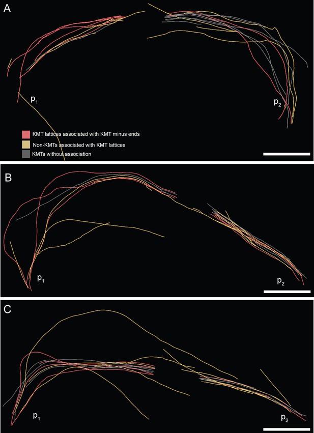
Association of KMT lattices with other MT minus ends at an interaction distance of 35 nm.
(A) Visualization of KMTs and non-KMTs obtained from the ASGA 3D-Viewer (https://cfci.shinyapps.io/ASGA_3DViewer) showing a k-fiber pair from spindle #1 (ASGA k-fiber ID: pole1_08 / pole2_08). This 3D model illustrates the association of KMT lattices with MT minus ends at an interaction distance of 35 nm. The types of interaction are shown by color-coding (top image). The approximated position of the spindle poles (p1, p2) is indicated. (B) Model of k-fiber pair with ID: pole1_20 / pole2_20. (C) Model of k-fiber pair with ID: pole1_23 / pole2_23. Scale bars, 1 µm.
Associations of KMT minus ends with MT lattices in spindle #1.
Three-dimensional model of all KMTs from spindle #1. KMT minus ends interacting with other MTs at association distances up to 35 nm are shown. KMT minus ends interacting with either KMT (red lines) or non-KMT lattices (yellow lines) are illustrated. KMTs without any interactions are shown in gray. This video corresponds to Figure 8—figure supplement 1. Scale bar, 1 µm.
Association of KMT minus end with MT lattices.
Three-dimensional model of KMTs from spindle #1 (ASGA k-fiber ID: pole1_08). The association of KMT minus-end with other MTs is shown. The distance of interaction is 35 nm. KMT minus-end association with either KMTs (purple lines) or non-KMT lattices (yellow lines) is indicated. KMTs without any association are shown in gray. This video corresponds to Figure 8—figure supplement 1. Scale bars, 1 µm.
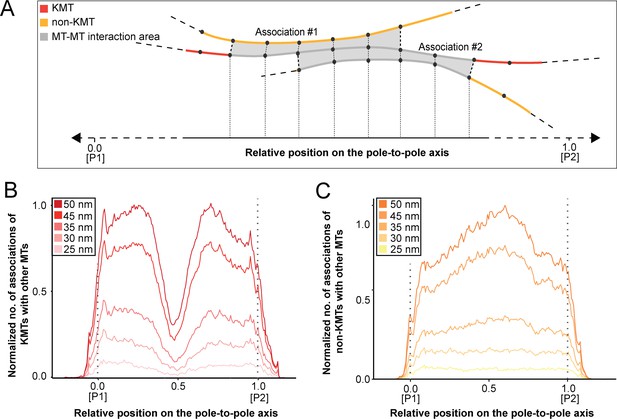
Positions of MT-MT associations.
(A) Schematic illustration showing the mapping of the number of MT-MT associations on the pole-to-pole axis (P1, position = 0; P2, position = 1). The number of associations is measured in defined segments (20 nm). KMTs are illustrated in red, non-KMTs in yellow, and areas of MT-MT association in gray. (B) Graph showing the number of KMTs associated with other MTs plotted against the relative position on the pole-to-pole axis. KMT number is normalized by the MT density. The defined association distances for KMTs with other MTs in the spindle are given in the insert. (C) Number of non-KMTs associated with neighboring MTs plotted against the relative position on the pole-to-pole axis.
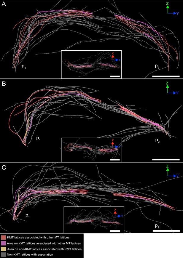
Association of KMT lattices with other MT lattices at an interaction distance of 35 nm.
(A) Visualization of KMTs and non-KMTs obtained from the ASGA 3D-Viewer (https://cfci.shinyapps.io/ASGA_3DViewer/) showing a k-fiber pair from spindle #1 (ASGA k-fiber ID: pole1_08). This 3D model illustrates the association of KMT lattices with other MT at an interaction distance of 35 nm. The types of association are shown by color-coding (bottom). Association areas are shown as yellow segments on each MT. The approximated position of the spindle poles (p1, p2) is indicated. The k-fiber pair is shown in a Z/Y (large image) and an X/Y view (insert). (B) Model of k-fiber pair with ID: pole1_20. (C) Model of k-fiber pair with ID: pole1_23. Scale bars, 1 µm.
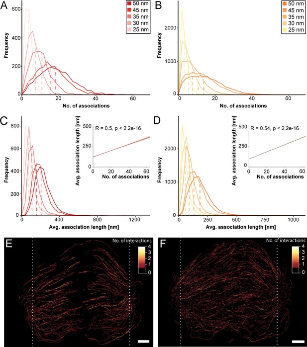
Association of KMT lattices with MT minus ends.
(A) Frequency of the number of associations of KMTs with other MTs in the spindle (n=2579). Plots are shown for five different interaction distances (insert). (B) Frequency of the number of associations of non-KMTs with other MTs (n=16256). (C) Frequency of the average length of KMT-MT associations per KMT (n=2579). The correlation of the average length of associations with the average number of associations is also given (insert). (D) Frequency of the average length of non-KMT-MT associations per non-KMT (n=16256). (E) Three-dimensional model of all KMTs showing regions of KMT-MT association within 35 nm of interaction or closer (n=2579). Each KMT segment is color-coded according to the number of associations (insert). (F) Three-dimensional model of all non-KMTs showing regions of MT-MT association within 35 nm of interaction or closer (n=16256). White dashed lines indicate the position of the spindle poles (E and F). Scale bars, 1 µm.
Associations of KMT lattices with other MTs.
Three-dimensional model of all KMTs in spindle #1. KMT lattices associated with other MT lattices at are shown. The distances of interaction is 35 nm. KMTs are shown as gray lines with color-coded regions indicating the number of MT-MT associations. This video corresponds to Figure 9—figure supplement 2E. Scale bar, 1 µm.
Associations of non-KMTs with other MTs.
Three-dimensional model of all non-KMTs in spindle #1. Non-KMT lattices associated with other MT lattices are shown. The distances of interaction is 35 nm. Non-KMTs are shown as gray lines with color-coded regions indicating the number of MT-MT associations. This video corresponds to Figure 9—figure supplement 2F. Scale bar, 1 µm.
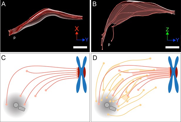
Model of a k-fiber showing a semi-direct connection between a kinetochore and a spindle pole.
(A–B) Three-dimensional views of a selected 3D-reconstructed k-fiber with an overlay area drawn around KMTs using the alpha shape method. The KMTs are shown as red lines and the ends are marked with red dots. The approximate position of the pole is indicated (p). The same k-fiber is shown from two different perspectives (X/Y view in A; Z/Y view in B). Scale bars, 1 µm. (C) Schematic model of a semi-direct connection between a kinetochore (chromosome in blue, paired kinetochores in dark red) and a spindle pole (MT-centrosome interaction area and centrioles in gray) as established by a single k-fiber. KMTs are shown as red lines, KMT ends as light red circles. (D) Model of the k-fiber (as shown in C) associated with the surrounding non-KMT network. Non-KMTs are shown as yellow lines, non-KMT ends as yellow circles. KMT-KMT interactions are indicated by light red areas, KMT-non-KMT interactions by light yellow areas.
Tables
Characterization of the 3D-reconstructed metaphase spindles in HeLa cells.
| Data set | Spindle pole distance [µm] | Inter-kinetochore distance [µm]* | No. of MTs in the tomographic volume | No. of kinetochores | No. of KMTs | No. of non-KMTs | No. of k-fibers |
|---|---|---|---|---|---|---|---|
| Spindle #1 | 7.16 | 1.08 ± 0.20 (n=43) | 4884 | 92 | 797 (16.3%) | 4087 (83.7%) | 92 |
| Spindle #2 | 10.39 | 1.24 ± 0.21 (n=50) | 8047 | 110 | 1,102 (13.7%) | 6945 (86.3%) | 110 |
| Spindle #3 | 9.48 | 1.03 ± 0.27 (n=40) | 5904 | 90 | 680 (11.5%) | 5224 (88.5%) | 90 |
-
*
Numbers are given as mean ± STD.
Tomographic data sets as used throughout this study.
| Data set | Original data set | Montage (X/Y) | No. of serial sections[300 nm each] | Estimated tomographic volume [µm3] | Data set size [Gb] |
|---|---|---|---|---|---|
| Spindle #1 | T_0475 | 2 × 3 | 22 | 598 | 46.5 |
| Spindle #2 | T_0479 | 2 × 3 | 29 | 996 | 77.9 |
| Spindle #3 | T_0494 | 2 × 3 | 35 | 904 | 71.9 |
Quantitative analysis of KMTs and non-KMTs.
| Data set | Length of KMTs [µm]* | Length of non- KMTs [µm]* | No. of KMTs per kinetochore* | No. of KMTs in the MT-centrosome interaction area* | Mean KMT minus-end distance to poles [µm] | % of KMTs associated with poles | % of non-KMTs associated with poles |
|---|---|---|---|---|---|---|---|
| Spindle #1 | 3.59 (±1.57) | 2.13 (±1.67) | 8.04 (±1.86) | 5.0 (±1.8) | 1.72 | 61.2 | 44.3 |
| Spindle #2 | 3.82 (±1.97) | 1.95 (±1.60) | 9.75 (±2.18) | 3.1 (±2.3) | 2.87 | 31.5 | 28.6 |
| Spindle #3 | 4.27 (±1.93) | 2.07 (±1.93) | 7.49 (±1.91) | 4.1 (±2.0) | 2.12 | 54.2 | 41.9 |
-
*
Numbers are given as mean ±STD.
Quantitative analysis of k-fiber organization.
| Data set | KMT density at the kinetochore [KMT/µm2]* | KMT-KMT distance at the kinetochore [nm]* | Global tortuosity of KMTs* | % of curved KMTs | Area of k-fibers [µm2]* | % of KMTs in a k-fibers* |
|---|---|---|---|---|---|---|
| Spindle #1 | 122 (±62) | 67 (±20) | 1.11 (±0.11) | 39.8 | 0.08 (±0.1) | 64 (±27) |
| Spindle #2 | 99 (±45) | 78 (±23) | 1.07 (±0.07) | 28.4 | 0.09 (±0.11) | 70 (±25) |
| Spindle #3 | 117 (±72) | 76 (±23) | 1.13 (±0.13) | 47.1 | 0.12 (±0.24) | 59 (±29) |
-
*
Numbers are given as mean ±STD.
Quantitative analysis of k-fiber positioning in the spindle.
| Region | Length of KMTs [µm]* | No. of KMTs per kinetochore* | No. of KMTs at MT-centrosome interaction area† | Mean KMT minus-end distance to poles [µm]* | No. of KMTs associated with poles* | Global tortuosity of KMTs* |
|---|---|---|---|---|---|---|
| Central | 3.5 (±1.7) | 8.2 (±2.4) | 162 (~48%) | 2.0 (±1.3) | 4.3 (±2.3) | 1.08 (±0.08) |
| Intermediate | 3.6 (±1.7) | 8.6 (±2.1) | 266 (~49%) | 2.1 (±1.3) | 4.6 (±1.9) | 1.11 (±0.12) |
| Peripheral | 3.9 (±2.0) | 8.6 (±2.4) | 730 (~45%) | 2.5 (±1.6) | 4.1 (±2.0) | 1.10 (±0.10) |
-
*
Numbers are given as mean ±STD.
-
†
Number and percentage of KMTs is shown.
Analysis of the association of KMT minus ends with other neighboring KMT lattices.
| Data set | Analysis | Interaction distances [nm] | ||||||
|---|---|---|---|---|---|---|---|---|
| 25 | 30 | 35 | 45 | 50 | 75 | 100 | ||
| Spindle #1 | No. of KMTs | 37 | 68 | 112 | 204 | 238 | 306 | 330 |
| % of KMTs | 4.9 | 9.1 | 15.0 | 27.3 | 32.0 | 40.9 | 44.1 | |
| Spindle #2 | No. of KMTs | 20 | 37 | 68 | 142 | 177 | 266 | 290 |
| % of KMTs | 1.9 | 3.5 | 6.3 | 13.2 | 16.5 | 24.8 | 27.1 | |
| Spindle #3 | No. of KMTs | 13 | 27 | 66 | 116 | 135 | 199 | 218 |
| % of KMTs | 1.9 | 4.0 | 9.8 | 17.2 | 20.0 | 29.5 | 32.3 | |
Analysis of the association of KMT minus ends with neighboring non-KMT lattices.
| Data set | Analysis | Interaction distances [nm] | ||||||
|---|---|---|---|---|---|---|---|---|
| 25 | 30 | 35 | 45 | 50 | 75 | 100 | ||
| Spindle #1 | No. of KMTs | 37 | 82 | 132 | 217 | 248 | 353 | 384 |
| % of KMTs | 4.9 | 11.0 | 17.6 | 29.0 | 33.2 | 47.2 | 51.3 | |
| Spindle #2 | No. of KMTs | 245 | 313 | 353 | 469 | 525 | 677 | 732 |
| % of KMTs | 22.9 | 29.2 | 33.0 | 43.8 | 49.0 | 63.2 | 68.3 | |
| Spindle #3 | No. of KMTs | 28 | 64 | 107 | 198 | 230 | 355 | 410 |
| % of KMTs | 4.2 | 9.5 | 15.9 | 29.4 | 34.1 | 52.7 | 60.8 | |
Analysis of the association of KMT lattices with other neighboring KMT minus ends.
| Data set | Analysis | Interaction distances [nm] | ||||||
|---|---|---|---|---|---|---|---|---|
| 25 | 30 | 35 | 45 | 50 | 75 | 100 | ||
| Spindle #1 | No. of KMTs | 39 | 71 | 117 | 210 | 236 | 336 | 403 |
| % of KMTs | 5% | 10% | 15% | 28% | 31% | 45% | 54% | |
| Spindle #2 | No. of KMTs | 24 | 46 | 86 | 179 | 237 | 401 | 470 |
| % of KMTs | 2% | 4% | 8% | 17% | 22% | 37% | 43% | |
| Spindle #3 | No. of KMTs | 14 | 27 | 61 | 127 | 148 | 227 | 284 |
| % of KMTs | 2% | 4% | 9% | 19% | 22% | 34% | 43% | |
Analysis of the association of KMT lattices with other neighboring non-KMT minus ends.
| Data set | Analysis | Interaction distances [nm] | ||||||
|---|---|---|---|---|---|---|---|---|
| 25 | 30 | 35 | 45 | 50 | 75 | 100 | ||
| Spindle #1 | No. of KMTs | 81 | 151 | 223 | 362 | 415 | 534 | 577 |
| % of KMTs | 11% | 20% | 30% | 48% | 55% | 71% | 77% | |
| Spindle #2 | No. of KMTs | 51 | 100 | 173 | 351 | 433 | 640 | 717 |
| % of KMTs | 5% | 9% | 16% | 33% | 40% | 59% | 67% | |
| Spindle #3 | No. of KMTs | 34 | 93 | 176 | 301 | 348 | 471 | 507 |
| % of KMTs | 5% | 14% | 26% | 44% | 51% | 69% | 75% | |
Average number of associations of KMTs and non-KMTs with MT lattices.
| Data set | MT type | Interaction distances [nm] | ||||
|---|---|---|---|---|---|---|
| 25 | 30 | 35 | 45 | 50 | ||
| Spindle #1* | KMTs | 4.8 (±1.5) | 8.6 (±2.5) | 12.4 (±3.4) | 18.8 (±4.9) | 1.3 (±5.5) |
| Non-KMTs | 4.4 (±1.5) | 7.0 (±2.6) | 9.6 (±3.7) | 13.0 (±5.4) | 16.2 (±6.2) | |
| Spindle #2* | KMTs | 4.2 (±1.3) | 5.8 (±1.8) | 8.0 (±2.6) | 13.3 (±4.1) | 16.0 (±4.8) |
| Non-KMTs | 3.2 (±0.9) | 4.0 (±1.3) | 5.2 (±1.8) | 8.2 (±3.1) | 9.8 (±3.7) | |
| Spindle #3* | KMTs | 4.2 (±1.2) | 8.0 (±2.3) | 12.4 (±3.4) | 18.6 (±4.8) | 21.2 (±5.4) |
| Non-KMTs | 3.6 (±1.2) | 5.2 (±2.3) | 8.0 (±3.3) | 11.6 (±4.7) | 13.2 (±5.3) | |
| All spindles* | KMTs | 4.4 (±1.3) | 7.4 (±2.3) | 10.6 (±3.2) | 16.4 (±4.7) | 19.0 (±5.3) |
| Non-KMTs | 3.6 (±1.2) | 5.4 (±2.2) | 7.4 (±3.1) | 10.8 (±4.5) | 12.4 (±5.1) | |
-
*
Numbers are given as mean ±STD.
Average length of associations of KMTs and non-KMTs with MT lattices.
| Data set | MT type | Interaction distances [nm] | ||||
|---|---|---|---|---|---|---|
| 25 | 30 | 35 | 45 | 50 | ||
| Spindle #* | KMTs | 81.3 (±88.8) | 119.7 (±151.1) | 163.9 (±207.5) | 241.3 (±301.9) | 271.0 (±335.9) |
| Non-KMTs | 58.3 (±54.1) | 78.3 (±79.9) | 107.7 (±116.9) | 165.1 (±195.1) | 187.9 (±227.0) | |
| Spindle #2* | KMTs | 69.5 (±69.9) | 93.2 (±107.0) | 124.3 (±146.0) | 207.8 (±252.3) | 252.2 (±314,9) |
| Non-KMTs | 59.2 (±53.2) | 73.2 (±71.9) | 92.3 (±97.3) | 145.8 (±170.5) | 175.1 (±213.0) | |
| Spindle #3* | KMTs | 66.1 (±63.4) | 97.3 (±117.8) | 143.2 (±191.7) | 231.3 (±321.2) | 263.4 (±362.2) |
| Non-KMTs | 54.3 (±51.7) | 74.5 (±86.4) | 104.6 (±133.7) | 165.6 (±218.7) | 191.3 (±252.0) | |
| All spindles* | KMTs | 73.0 (±76.2) | 104.6 (±129.2) | 145.1 (±186.0) | 225.6 (±292.3) | 261.9 (±336.8) |
| Non-KMTs | 57.2 (±53.1) | 75.4 (±80.5) | 102.2 (±118.9) | 159.1 (±197.2) | 184.9 (±232.1) | |
-
*
Numbers are given as mean ±STD.
| Reagent type (species) or resource | Designation | Source or reference | Identifiers | Additional information |
|---|---|---|---|---|
| Strain, background (HeLa, Kyoto) | Gerlich Lab | IMBA, Vienna, Austria | - | - |
| Software, algorithm | SerialEM Boulder Laboratory for 3-Dimensional Electron Microscopy of cells Colorado, USA | https://bio3d.colorado.edu/ Mastronarde, 2003 | - | - |
| Software, algorithm | IMOD Boulder Laboratory for 3-Dimensional Electron Microscopy of cells Colorado, USA | http://bio3d.colorado.edu/ Kremer et al., 1996 | - | - |
| Software, algorithm | Amira Thermo Fisher Scientific, USA | https://www.zib.de/software/amira Stalling et al., 2005 | - | - |
| Software, algorithm | ASGA Robert Kiewisz / Müller - Reichert Lab Dresden, Germany | https://github.com/RRobert92/ Kiewisz and Müller-Reichert, 2021 | - | https://kiewisz.shinyapps.io/ASGA |
| Software, algorithm | ASGA - 3D Viewer Robert Kiewisz / Müller - Reichert Lab Dresden, Germany | https://github.com/RRobert92/ Kiewisz and Müller-Reichert, 2022 | - | https://cfci.shinyapps.io/ASGA_3DViewer/ |
Quantification of KMT ultrastructure before and after application of Z-expansion to the 3D models.
| Data set | Length of KMTs [µm]* | Length of non- KMTs [µm]* | No. of KMTs per kinetochore* | No. of KMTs in the MT-centrosome interaction area* | Mean KMT minus-end distance to poles [µm] | No. of KMTs associated with poles [%] | No. of non-KMTs associated with poles [%] | |||||||
|---|---|---|---|---|---|---|---|---|---|---|---|---|---|---|
| Before | After | Before | After | Before | After | Before | After | Before | After | Before | After | Before | After | |
| Spindle #1 | 3.23 (±1.49) | 3.59 (±1.57) | 2.03 (±1.6) | 2.13 (±1.67) | 8.04 (±1.86) | 8.04 (±1.86) | 4.1 (±1.8) | 5.0 (±1.8) | 1.16 | 1.72 | 62.2 | 61.2 | 44.5 | 44.3 |
| Spindle #2 | 3.69 (±1.87) | 3.82 (±1.97) | 1.85 (±1.55) | 1.95 (±1.60) | 9.75 (±2.18) | 9.75 (±2.18) | 2.4 (±2.0) | 3.1 (±2.3) | 2.47 | 2.87 | 53.6 | 31.5 | 28.8 | 28.6 |
| Spindle #3 | 4.03 (±1.79) | 4.27 (±1.93) | 1.91 (±1.80) | 2.07 (±1.93) | 7.49 (±1.91) | 7.49 (±1.91) | 3.4 (±1.8) | 4.1 (±2.0) | 1.35 | 2.12 | 62.0 | 54.2 | 42.3 | 41.9 |
-
*
Numbers are given as mean ±STD.
Quantification of k-fiber organization before and after application of Z-expansion to the 3D models.
| Data set | Density of KMTs at the kinetochore [KMT/µm2]* | KMT-KMT distance at the kinetochore [nm]* | Global tortuosity of KMTs* | % of curved KMTs* | Area of k-fibers [µm2]* | % of KMTs in a k-fibers* | ||||||
|---|---|---|---|---|---|---|---|---|---|---|---|---|
| Before | After | Before | After | Before | After | Before | After | Before | After | Before | After | |
| Spindle #1 | 151 (±74) | 122 (±62) | 61 (±11) | 67 (±20) | 1.09 (±0.10) | 1.11 (±0.11) | 36.1 | 39.8 | 0.063 (±0.09) | 0.08 (±0.1) | 34 (±27) | 64 (±27) |
| Spindle #2 | 137 (±68) | 99 (±45) | 65 (±12) | 78 (±23) | 1.06 (±0.06) | 1.07 (±0.07) | 21.4 | 28.4 | 0.068 (±0.10) | 0.09 (±0.11) | 70 (±25) | 70 (±25) |
| Spindle #3 | 175 (±123) | 117 (±72) | 66 (±12) | 76 (±23) | 1.11 (±0.11) | 1.13 (±0.13) | 39.5 | 47.1 | 0.080 (±0.15) | 0.12 (±0.24) | 59 (±39) | 59 (±29) |
-
*
Numbers are given as mean ±STD.


