Rapid, Reference-Free human genotype imputation with denoising autoencoders
Figures
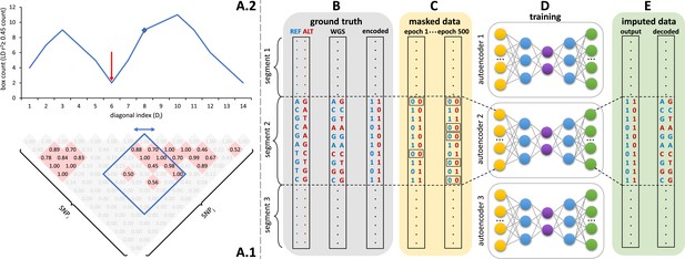
Schematic overview of the autoencoder training workflow.
(A) Tiling of autoencoders across the genome is achieved by (A.1) calculating a n x n matrix of pairwise SNP correlations, thresholding them at 0.45 (selected values are shown in red background, excluded values in gray), (A.2) quantifying the overall local LD strength centered at each SNP by computing their local correlation box counts and splitting the genome into approximately independent segments by identifying local minima (recombination hotspots). The red arrow illustrates minima between strong LD regions. For reducing computational complexity, we calculated the correlations in a fixed sliding box size of 500x500 common variants (MAF ≥ 0.5%). Thus, the memory utilization for calculating correlations will be the same regardless of genomic density. (B) Ground truth whole genome sequencing data is encoded as binary values representing the presence (1) or absence (0) of the reference allele (blue) and alternative allele (red). (C) Variant masking (setting both alleles as absent, represented by 0, corrupts data inputs at a gradually increasing masking rate). Example masked variants are outlined. (D) Fully-connected autoencoders spanning segments defined as shown in panel (A), are then trained to reconstruct the original uncorrupted data from corrupted inputs; (E) the reconstructed outputs (imputed data) are compared to the ground truth states for loss calculation and are decoded back to genotypes.
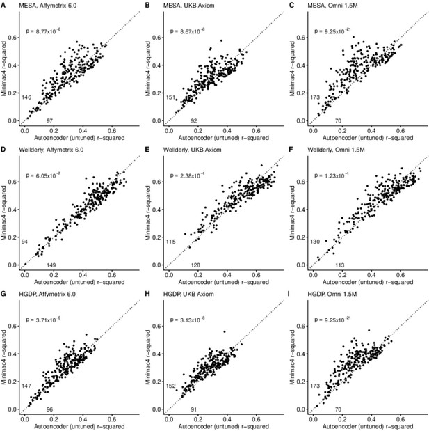
HMM-based (y-axis) versus autoencoder-based (x-axis) imputation accuracy prior to tuning.
Minimac4 and untuned autoencoders were tested across three independent datasets–- MESA (top), Wellderly (middle), and HGDP (bottom) and across three genotyping array platforms–- Affymetrix 6.0 (left), UKB Axiom (middle), Omni1.5M (right). Each data point represents the imputation accuracy (average r-squared per variant) for an individual genomic segment relative to its WGS-based ground truth. The numerical values presented on the left side and below the identity line (dashed line) indicate the number of genomic segments in which Minimac4 outperformed the untuned autoencoder (left of identity line) and the number of genomic segments in which the untuned autoencoder surpassed Minimac4 (below the identity line). Statistical significance was assessed through two-proportion Z-test p-values.
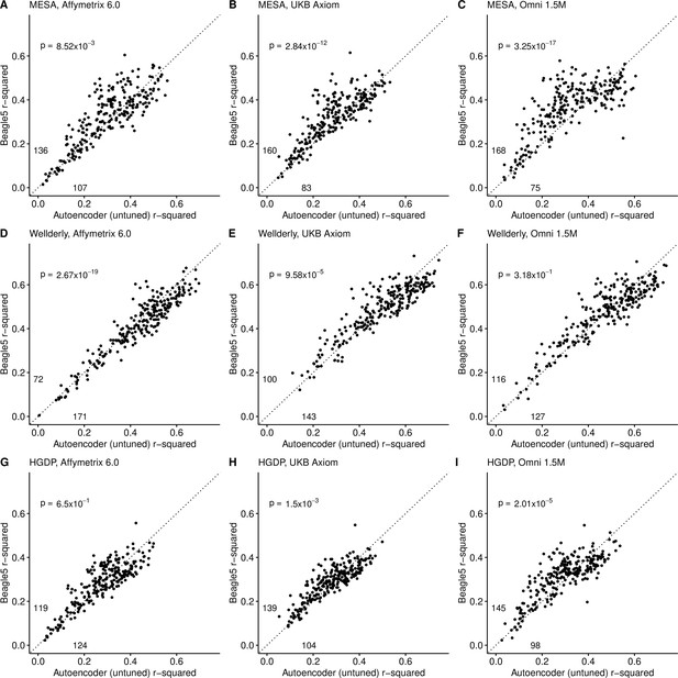
Beagle5 (y-axis) versus autoencoder-based (x-axis) imputation accuracy prior to tuning.
Beagle5 and untuned autoencoders were tested across three independent datasets - MESA (top), Wellderly (middle), and HGDP (bottom) and across three genotyping array platforms - Affymetrix 6.0 (left), UKB Axiom (middle), Omni1.5M (right). Each data point represents the imputation accuracy (average r-squared per variant) for an individual genomic segment relative to its WGS-based ground truth. The numerical values presented on the left side and below the identity line (dashed line) indicate the number of genomic segments in which Beagle5 outperformed the untuned autoencoder (left of identity line) and the number of genomic segments in which the untuned autoencoder surpassed Beagle5 (below the identity line). Statistical significance was assessed through two-proportion Z-test p-values.
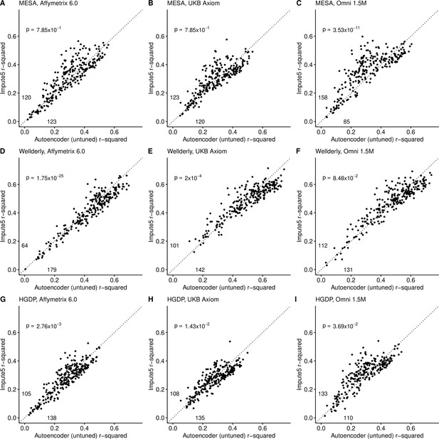
Impute5 (y-axis) versus autoencoder-based (x-axis) imputation accuracy prior to tuning.
Impute5 and untuned autoencoders were tested across three independent datasets - MESA (top), Wellderly (middle), and HGDP (bottom) and across three genotyping array platforms - Affymetrix 6.0 (left), UKB Axiom (middle), Omni1.5M (right). Each data point represents the imputation accuracy (average r-squared per variant) for an individual genomic segment relative to its WGS-based ground truth. The numerical values presented on the left side and below the identity line (dashed line) indicate the number of genomic segments in which Impute5 outperformed the untuned autoencoder (left of identity line) and the number of genomic segments in which the untuned autoencoder surpassed Impute5 (below the identity line). Statistical significance was assessed through two-proportion Z-test p-values.
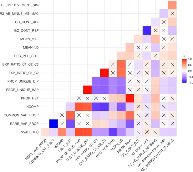
Relationship between genomic segment features and autoencoder performance.
Spearman correlations (ρ) between genomic segment features and autoencoder performance metrics are presented. An “X” denotes Spearman correlations that are not statistically significant (p>0.05). The performance metrics include the mean validation accuracy of Minimac4 and autoencoder (R2_AE_MINUS_MINIMAC), the autoencoder’s improvement in accuracy observed after offspring formation (AE_IMPROVEMENT_SIM) and the autoencoder’s improvement in accuracy after fine tuning of hyperparameters (AE_IMPROVEMENT_TUNING). The genomic features include the total number of variants per genomic segment in HRC (NVAR_HRC), proportion of rare variants at MAF ≤0.5% threshold (RARE_VAR_PROP), proportion of common variants at MAF >0.5% threshold (COMMON_VAR_PROP), number of components needed to explain at least 90% of variance after running Principal Component Analysis (NCOMP), proportion of heterozygous genotypes (PROP_HET), proportion of unique haplotypes (PROP_UNIQUE_HAP) and diplotypes (PROP_UNIQUE_DIP), sum of ratios of explained variance from first two (EXP_RATIO_C1_C2) and three (EXP_RATIO_C1_C2_C3) components from Principal Component Analysis, recombination per variant per variant (REC_PER_SITE), mean pairwise correlation across all variants in each genomic segment (MEAN_LD), mean MAF (MEAN_MAF), GC content of reference alleles (GC_CONT_REF), GC content of alternate alleles (GC_CONT_ALT).
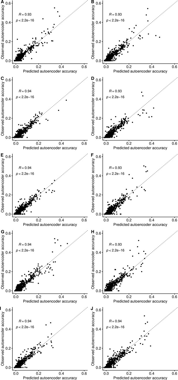
Projecting autoencoder performance from hyperparameters and genomic features.
We developed an ensemble-based machine learning approach (Extreme Gradient Boosting - XGBoost) to predict the expected performance (r-squared) of each hyperparameter combination per genomic segment using the results of the coarse-grid search and predictive features calculated for each genomic segment (see Materials and methods). We plot the observed accuracy of trained autoencoders versus the accuracy predicted by the XGBoost model after 10-fold cross-validation. Each subplot shows one iteration of the 10-fold validation process and its respective Pearson correlation between the predicted and observed accuracy values in the ARIC validation dataset.
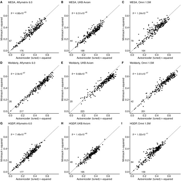
HMM-based (y-axis) versus autoencoder-based (axis) imputation accuracy after tuning.
Minimac4 and tuned autoencoders were validated across three independent datasets–- MESA (top), Wellderly (middle), and HGDP (bottom) and across three genotyping array platforms–- Affymetrix 6.0 (left), UKB Axiom (middle), Omni1.5M (right). Each data point represents the imputation accuracy (average r-squared per variant) for an individual genomic segment relative to its WGS-based ground truth. The numerical values presented on the left side and below the identity line (dashed line) indicate the number of genomic segments in which Minimac4 outperformed the untuned autoencoder (left of identity line) and the number of genomic segments in which the untuned autoencoder surpassed Minimac4 (below the identity line). Statistical significance was assessed through two-proportion Z-test p-values.
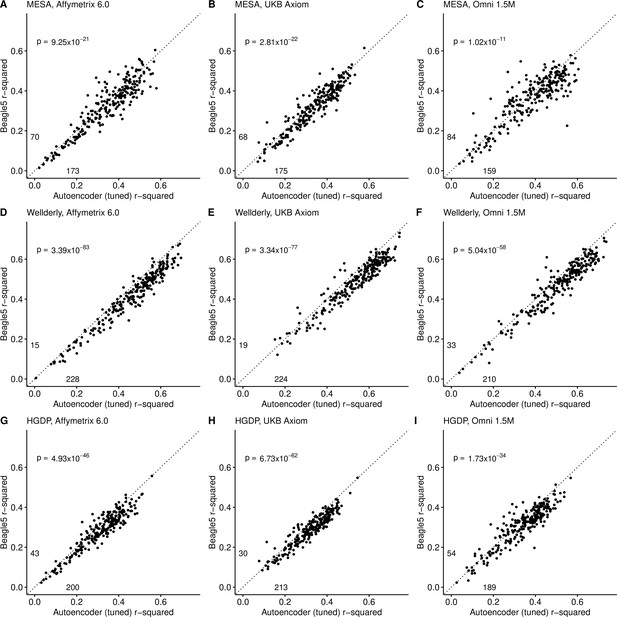
Beagle5 (y-axis) versus autoencoder-based (axis) imputation accuracy after tuning.
Beagle5 and tuned autoencoders were validated across three independent datasets - MESA (top), Wellderly (middle), and HGDP (bottom) and across three genotyping array platforms - Affymetrix 6.0 (left), UKB Axiom (middle), Omni1.5M (right). Each data point represents the imputation accuracy (average r-squared per variant) for an individual genomic segment relative to its WGS-based ground truth. The numerical values presented on the left side and below the identity line (dashed line) indicate the number of genomic segments in which Beagle5 outperformed the untuned autoencoder (left of identity line) and the number of genomic segments in which the untuned autoencoder surpassed Beagle5 (below the identity line). Statistical significance was assessed through two-proportion Z-test p-values.
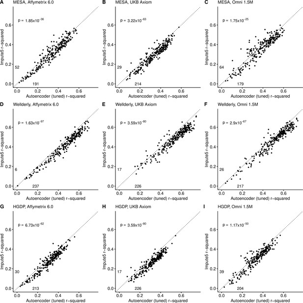
Impute5 (y-axis) versus autoencoder-based (axis) imputation accuracy after tuning.
Impute5 and tuned autoencoders were validated across three independent datasets - MESA (top), Wellderly (middle), and HGDP (bottom) and across three genotyping array platforms - Affymetrix 6.0 (left), UKB Axiom (middle), Omni1.5M (right). Each data point represents the imputation accuracy (average r-squared per variant) for an individual genomic segment relative to its WGS-based ground truth. The numerical values presented on the left side and below the identity line (dashed line) indicate the number of genomic segments in which Impute5 outperformed the untuned autoencoder (left of identity line) and the number of genomic segments in which the untuned autoencoder surpassed Impute5 (below the identity line). Statistical significance was assessed through two-proportion Z-test p-values.
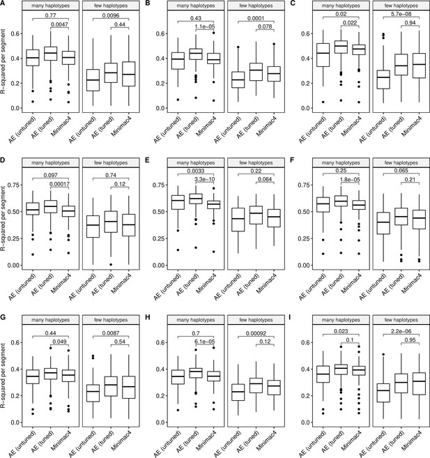
Imputation accuracy as a function of unique haplotype abundance.
Minimac4 and tuned and untuned autoencoders (AE) were tested across three independent datasets - MESA (top), Wellderly (middle), and HGDP (bottom) and across three genotyping array platforms - Affymetrix 6.0 (left), UKB Axiom (middle), Omni1.5M (right). ‘Many’ vs ‘Few’ haplotypes are defined by splitting genomic segments into those with greater than vs less than the median number of unique haplotypes per genomic segment. We applied Wilcoxon rank-sum tests to compare the untuned and tuned autoencoder to Minimac4. The validation datasets consist of: (A) MESA Affymetrix 6.0; (B) MESA UKB Axiom; (C) MESA Omni 1.5 M; (D) Wellderly Affymetrix 6.0; (E) Wellderly UKB Axiom; (F) Wellderly Omni 1.5 M; (G) HGDP Affymetrix 6.0; (H) HGDP UKB Axiom; (I) HGDP Omni 1.5 M.
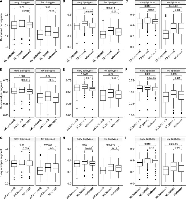
Imputation accuracy as a function of unique diplotype abundance.
Minimac4 and tuned and untuned autoencoders (AE) were tested across three independent datasets - MESA (top), Wellderly (middle), and HGDP (bottom) - and across three genotyping array platforms - Affymetrix 6.0 (left), UKB Axiom (middle), Omni1.5M (right). ‘Many’ vs ‘Few’ diplotypes are defined by splitting genomic segments into those with greater than vs less than the median number of unique diplotypes per genomic segment. We applied Wilcoxon rank-sum tests to compare the untuned and tuned autoencoder to Minimac4. The validation datasets consist of: (A) MESA Affymetrix 6.0; (B) MESA UKB Axiom; (C) MESA Omni 1.5 M; (D) Wellderly Affymetrix 6.0; (E) Wellderly UKB Axiom; (F) Wellderly Omni 1.5 M; (G) HGDP Affymetrix 6.0; (H) HGDP UKB Axiom; (I) HGDP Omni 1.5 M.
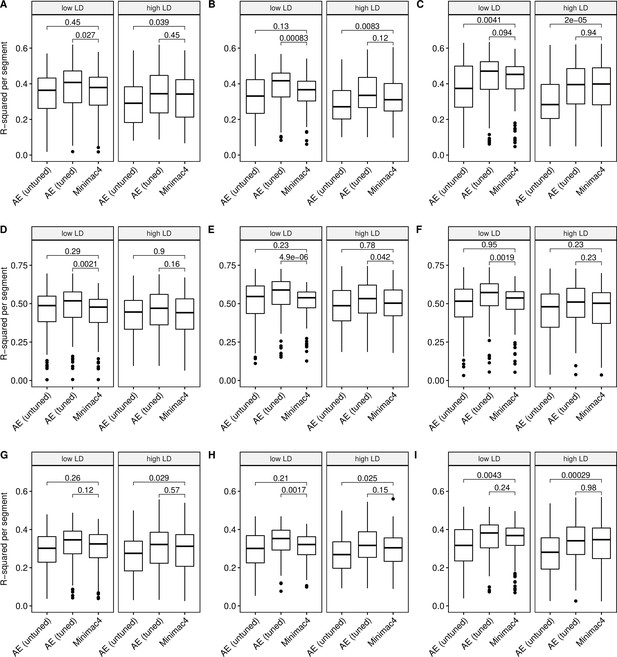
Imputation accuracy as a function of linkage disequilibrium (LD).
Minimac4 and tuned and untuned autoencoders (AE) were tested across three independent datasets - MESA (top), Wellderly (middle), and HGDP (bottom) - and across three genotyping array platforms - Affymetrix 6.0 (left), UKB Axiom (middle), Omni1.5M (right). ‘High’ vs ‘Low’ LD is defined by splitting genomic segments into those with greater than vs less than the average pairwise LD strength per genomic segment. We applied Wilcoxon rank-sum tests to compare the untuned and tuned autoencoder to Minimac4. The validation datasets consist of: (A) MESA Affymetrix 6.0; (B) MESA UKB Axiom; (C) MESA Omni 1.5 M; (D) Wellderly Affymetrix 6.0; (E) Wellderly UKB Axiom; (F) Wellderly Omni 1.5 M; (G) HGDP Affymetrix 6.0; (H) HGDP UKB Axiom; (I) HGDP Omni 1.5 M.
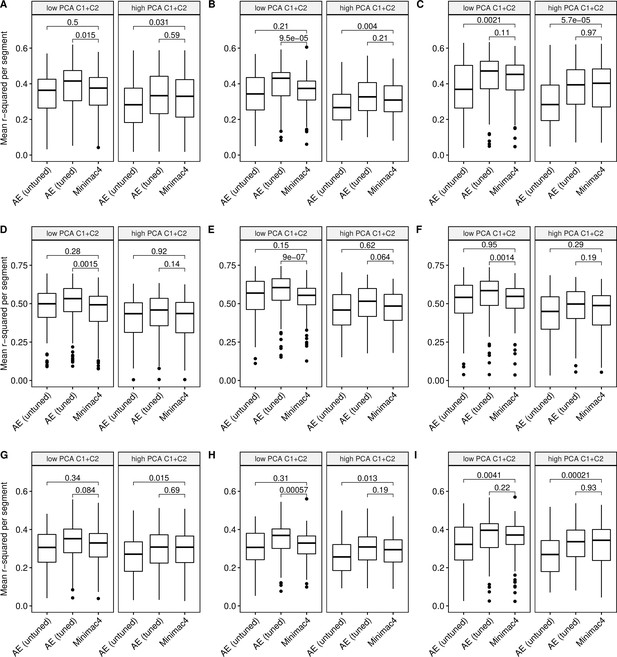
Imputation accuracy as a function of data complexity.
Minimac4 and tuned and untuned autoencoders (AE) were tested across three independent datasets - MESA (top), Wellderly (middle), and HGDP (bottom) - and across three genotyping array platforms - Affymetrix 6.0 (left), UKB Axiom (middle), Omni1.5M (right). ‘High’ vs ‘Low’ data complexity is defined by splitting genomic segments into those with greater than vs less than the median proportion of variance explained by first two components of Principal Component Analysis per genomic segment (PCA C1+C2). We applied Wilcoxon rank-sum tests to compare the untuned and tuned autoencoder to Minimac4. The validation datasets consist of: (A) MESA Affymetrix 6.0; (B) MESA UKB Axiom; (C) MESA Omni 1.5 M; (D) Wellderly Affymetrix 6.0; (E) Wellderly UKB Axiom; (F) Wellderly Omni 1.5 M; (G) HGDP Affymetrix 6.0; (H) HGDP UKB Axiom; (I) HGDP Omni 1.5 M.
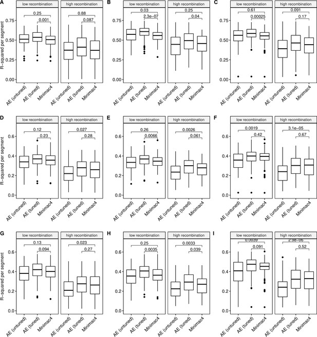
Imputation accuracy as a function of recombination rate.
Minimac4 and tuned and untuned autoencoders (AE) were tested across three independent datasets - MESA (top), Wellderly (middle), and HGDP (bottom) - and across three genotyping array platforms - Affymetrix 6.0 (left), UKB Axiom (middle), Omni1.5M (right). ‘High’ vs ‘Low’ recombination rate is defined by splitting genomic segments in those with greater than vs less than the median recombination rate per variant per genomic segment. We applied Wilcoxon rank-sum tests to compare the untuned and tuned autoencoder to Minimac4. The validation datasets consist of: (A) MESA Affymetrix 6.0; (B) MESA UKB Axiom; (C) MESA Omni 1.5 M; (D) Wellderly Affymetrix 6.0; (E) Wellderly UKB Axiom; (F) Wellderly Omni 1.5 M; (G) HGDP Affymetrix 6.0; (H) HGDP UKB Axiom; (I) HGDP Omni 1.5 M.
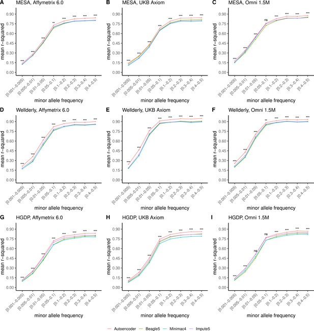
HMM-based versus autoencoder-based imputation accuracy across MAF bins.
Autoencoder-based (red) and HMM-based (Minimac4 (blue), Beagle5 (green), and Impute5 (purple)) imputation accuracy was validated across three independent datasets–- MESA (top), Wellderly (middle), and HGDP (bottom) and across three genotyping array platforms–- Affymetrix 6.0 (left), UKB Axiom (middle), Omni1.5M (right). Each data point represents the imputation accuracy (average r-squared per variant) relative to WGS-based ground truth across MAF bins. Error bars represent standard errors. We applied Wilcoxon rank-sum tests to compare the HMM-based tools to the tuned autoencoder (AE). * represents p-values ≤0.05, ** indicates p-values ≤0.001, and *** indicates p-values ≤0.0001, ns represents non-significant p-values.
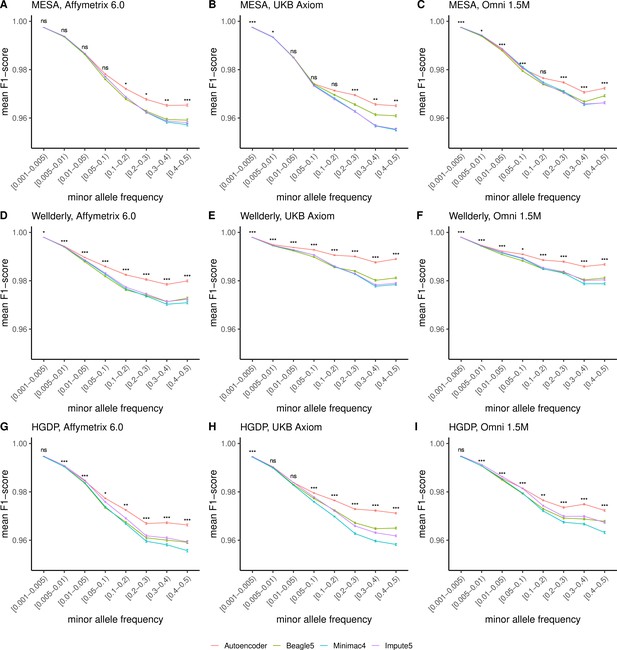
HMM-based versus autoencoder-based imputation accuracy across MAF bins (F1 score).
Autoencoder-based (red) and HMM-based (Minimac4 (blue), Beagle5 (green), and Impute5 (purple)) imputation accuracy was validated across three independent datasets - MESA (top), Wellderly (middle), and HGDP (bottom) - and across three genotyping array platforms - Affymetrix 6.0 (left), UKB Axiom (middle), Omni1.5M (right). Each data point represents the imputation accuracy (mean F1-score per variant) relative to WGS-based ground truth across MAF bins. Error bars represent standard errors. We applied Wilcoxon rank-sum tests to compare the HMM-based tools to the tuned autoencoder (AE). * represents p-values ≤0.05, ** indicates p-values ≤0.001, and *** indicates p-values ≤0.0001, ns represents non-significant p-values. Please note that F1 scores are high for rare variations given the high degree of class imbalance, most alternative alleles are not present for rare variants, leading to high accuracy in the negative class. R-squared depicted in Figure 4 provides a more accurate picture of balanced class accuracy.
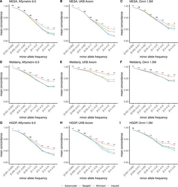
HMM-based versus autoencoder-based imputation accuracy across MAF bins (concordance).
Autoencoder-based (red) and HMM-based (Minimac4 (blue), Beagle5 (green), and Impute5 (purple)) imputation accuracy was validated across three independent datasets - MESA (top), Wellderly (middle), and HGDP (bottom) - and across three genotyping array platforms - Affymetrix 6.0 (left), UKB Axiom (middle), Omni1.5M (right). Each data point represents the imputation accuracy (mean concordance per variant) relative to WGS-based ground truth across MAF bins. Error bars represent standard errors. We applied Wilcoxon rank-sum tests to compare the HMM-based tools to the tuned autoencoder (AE). * represents p-values ≤0.05, ** indicates p-values ≤0.001, and *** indicates p-values ≤0.0001, ns represents non-significant p-values. Please note that F1 scores are high for rare variations given the high degree of class imbalance, most alternative alleles are not present for rare variants, leading to high accuracy in the negative class. R-squared depicted in Figure 4 provides a more accurate picture of balanced class accuracy.
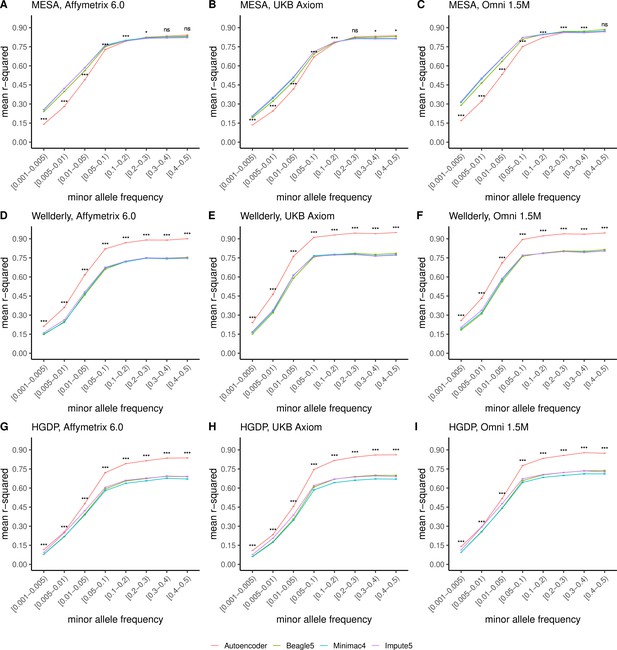
TOPMed cohort HMM-based imputation versus HRC cohort autoencoder-based imputation accuracy across MAF bins.
Autoencoder-based imputation using the HRC reference panel (red) was compared to HMM-based (Minimac4 (blue), Beagle5 (green), and Impute5 (purple)) imputation accuracy using the upgraded TOPMed cohort. Accuracy was determined across three datasets–- MESA (top – not independent), Wellderly (middle - independent), and HGDP (bottom - independent) and across three genotyping array platforms–- Affymetrix 6.0 (left), UKB Axiom (middle), Omni1.5M (right). Each data point represents the imputation accuracy (average r-squared per variant) relative to WGS-based ground truth across MAF bins. Error bars represent standard errors. We applied Wilcoxon rank-sum tests to compare the HMM-based tools to the tuned autoencoder (AE). * represents p-values ≤0.05, ** indicates p-values ≤0.001, and *** indicates p-values ≤0.0001, ns represents non-significant p-values.
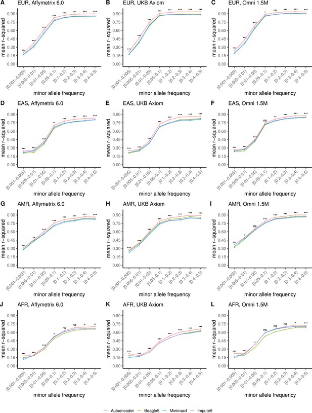
HMM-based versus autoencoder-based imputation accuracy across ancestry groups.
Autoencoder-based (red) and HMM-based (Minimac4 (blue), Beagle5 (green), and Impute5 (purple)) imputation accuracy was validated across individuals of diverse ancestry from MESA cohort (EUR: European (top); EAS: East Asian (2nd row); AMR: Native American (3rd row); AFR: African (bottom)) and multiple genotype array platforms (Affymetrix 6.0 (left), UKB Axiom (middle), Omni1.5M (right)). Each data point represents the imputation accuracy (average r-squared per variant) relative to WGS-based ground truth across MAF bins. Error bars represent standard errors. We applied Wilcoxon rank-sum tests to compare the HMM-based tools to the tuned autoencoder (AE). * represents p-values ≤0.05, ** indicates p-values ≤0.001, and *** indicates p-values ≤0.0001, ns represents non-significant p-values.
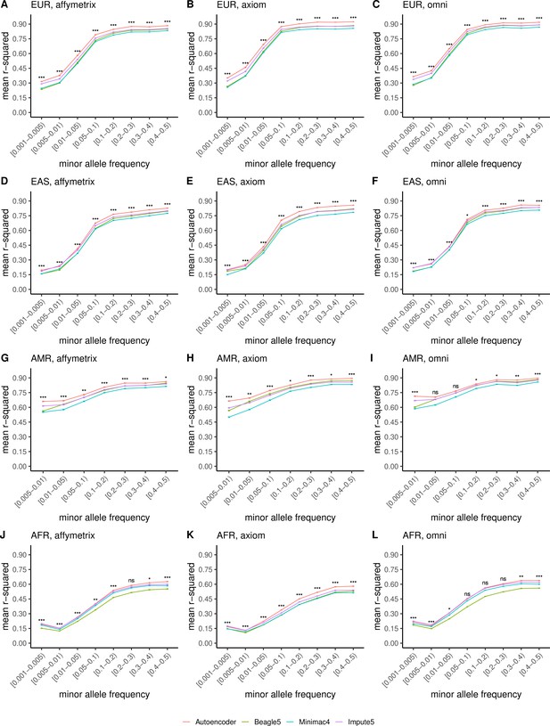
HMM-based versus autoencoder-based imputation accuracy across ancestry groups.
Autoencoder-based (red) and HMM-based (Minimac4 (blue), Beagle5 (green), and Impute5 (purple)) imputation accuracy was validated across individuals of diverse ancestry from HGDP cohort (EUR: European (top); EAS: East Asian (2nd row); AMR: Native American (3rd row); AFR: African (bottom)) and multiple genotype array platforms (Affymetrix 6.0 (left), UKB Axiom (middle), Omni1.5M (right)). Each data point represents the imputation accuracy (average r-squared per variant) relative to WGS-based ground truth across MAF bins. Error bars represent standard errors. We applied Wilcoxon rank-sum tests to compare the HMM-based tools to the tuned autoencoder (AE). * represents p-values ≤0.05, ** indicates p-values ≤0.001, and *** indicates p-values ≤0.0001, ns represents non-significant p-values.
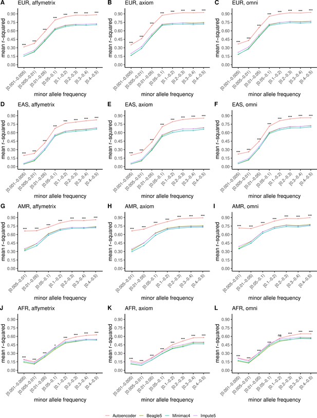
TOPMed cohort HMM-based versus HRC cohort autoencoder-based imputation accuracy across ancestry groups.
Autoencoder-based imputation using the HRC reference panel (red) was compared to HMM-based (Minimac4 (blue), Beagle5 (green), and Impute5 (purple)) imputation using the TOPMed reference panel. Accuracy was determined across individuals of diverse ancestry from the HGDP cohort (EUR: European (top); EAS: East Asian (2nd row); AMR: Native American (3rd row); AFR: African (bottom)) and multiple genotype array platforms (Affymetrix 6.0 (left), UKB Axiom (middle), Omni1.5M (right)). Each data point represents the imputation accuracy (average r-squared per variant) relative to WGS-based ground truth across MAF bins. Error bars represent standard errors. We applied Wilcoxon rank-sum tests to compare the HMM-based tools to the tuned autoencoder (AE). * represents p-values ≤0.05, ** indicates p-values ≤0.001, and *** indicates p-values ≤0.0001, ns represents non-significant p-values.
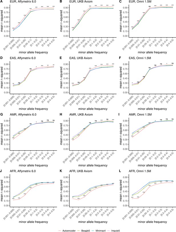
TOPMed cohort HMM-based versus HRC cohort autoencoder-based imputation accuracy across ancestry groups.
Autoencoder-based imputation using the HRC reference panel (red) was compared to HMM-based (Minimac4 (blue), Beagle5 (green), and Impute5 (purple)) imputation using the TOPMed reference panel. Accuracy was determined across individuals of diverse ancestry from the MESA cohort (EUR: European (top); EAS: East Asian (2nd row); AMR: Native American (3rd row); AFR: African (bottom)) and multiple genotype array platforms (Affymetrix 6.0 (left), UKB Axiom (middle), Omni1.5M (right)). Each data point represents the imputation accuracy (average r-squared per variant) relative to WGS-based ground truth across MAF bins. Error bars represent standard errors. We applied Wilcoxon rank-sum tests to compare the HMM-based tools to the tuned autoencoder (AE). * represents p-values ≤0.05, ** indicates p-values ≤0.001, and *** indicates p-values ≤0.0001, ns represents non-significant p-values.
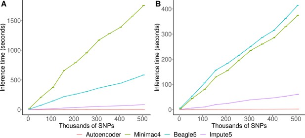
HMM-based versus autoencoder-based inference runtimes.
We plot the average time and standard error of three imputation replicates. Two hardware configurations were used for the tests: (A) a low-end environment: 16-core Intel Xeon CPU (E5-2640 v2 2.00 GHz), 250 GB RAM, and one GPU (NVIDIA GTX 1080); (B) a high-end environment: 24-Core AMD CPU (EPYC 7352 2.3 GHz), 250 GB RAM, using one NVIDIA A100 GPU.
Tables
Description and values of hyperparameters tested in grid search.
λ1: scaling factor for Least Absolute Shrinkage and Selection Operator (LASSO or L1) regularization; λ2: scaling factor for Ridge (L2) regularization; β: scaling factor for sparsity penalty described in Equation 4; ρ: target hidden layer activation described in Equation 4; Activation function type: defines how the output of a hidden neuron will be computed given a set of inputs; Learning rate: step size at each learning iteration while moving toward the minimum of the loss function; γ: amplifying factor for focal loss described in Equation 3; Optimizer type: algorithms utilized to minimize the loss function and update the model weights in backpropagation; Loss type: algorithms utilized to calculate the model error (Equation 2); Number of hidden layers: how many layers of artificial neurons to be implemented between input layer and output layer; Hidden layer size ratio: scaling factor to resize the next hidden layer with reference to the size of Its previous layer; Learning rate decay ratio: scaling factor for updating the learning rate value on every 500 epochs.
| Hyperparameter description | Tested values (coarse-grid search) |
|---|---|
| λ1 for L1 regularization | [1e-3, 1e-4, 1e-5, 1e-6, 1e-1, 1e-2, 1e-7, 1e-8] |
| λ2 for L2 regularization | [1e-3, 1e-4, 1e-5, 1e-6, 1e-1, 1e-2, 1e-7, 1e-8] |
| Sparsity scaling factor (β) | [0, 0.001, 0.01, 0.05, 1, 5, 10] |
| Target average hidden layer activation (ρ) | [0.001, 0.004, 0.007, 0.01, 0.04, 0.07, 0.1, 0.4, 0.7, 1.0] |
| Activation function type | [‘sigmoid’, ‘tanh’, ‘relu’, ‘softplus’] |
| Learning rate | [0.000001, 0.00001, 0.0001, 0.001, 0.01, 0.1, 1, 10, 100] |
| Amplifying factor for focal loss (γ) | [0, 0.5, 1, 2, 3, 5] |
| Optimizer type | [‘Adam’, ‘RMS Propagation’, ‘Gradient Descent’] |
| Loss type | [‘Binary Cross Entropy’, ‘Custom Focal Loss’] |
| Number of hidden layers | [1, 2, 4, 6, 8] |
| Hidden layer size ratio | [0.2, 0.3, 0.4, 0.5, 0.6, 0.7, 0.8, 0.9, 1] |
| Learning rate decay ratio | [ 0.0, 0.25, 0.5, 0.75, 0.95, 0.99, 0.999, 0.9999] |
Performance comparisons between untuned autoencoder (AE) and HMM-based imputation tools (Minimac4, Beagle5, and Impute5).
Average r-squared per variant was extracted from each genomic segment of chromosome 22. We applied Wilcoxon rank-sum tests to compare the HMM-based tools to the reference tuned autoencoder (AE). * represents p-values ≤0.05, ** indicates p-values ≤0.001, and *** indicates p-values ≤0.0001.
| MESA | Wellderly | HGDP | Affymetrix 6.0 | UKB Axiom | Omni 1.5 M | Combined | |
|---|---|---|---|---|---|---|---|
| AE (untuned) | 0.303±0.008 | 0.470±0.009 | 0.285±0.006 | 0.339±0.008 | 0.356±0.007 | 0.362±0.008 | 0.352±0.008 |
| Minimac4 | 0.337±0.007* | 0.471±0.008 | 0.314±0.006** | 0.352±0.008 | 0.370±0.006 | 0.400±0.007** | 0.374±0.007* |
| Beagle5 | 0.336±0.007* | 0.460±0.008 | 0.296±0.005 | 0.342±0.007 | 0.367±0.006 | 0.384±0.007* | 0.364±0.007 |
| Impute5 | 0.326±0.007* | 0.458±0.008 | 0.289±0.006 | 0.336±0.008 | 0.354±0.006 | 0.383±0.008* | 0.358±0.007 |
Top 10 best performing hyperparameter combinations that advanced to fine-tuning.
See Materials and methods and Table 1 for a detailed description of the hyperparameters.
| λ1 | λ2 | β | ρ | Activation | Learn rate | γ | Optimizer | Loss type | Hidden layers | Size ratio | Decay |
|---|---|---|---|---|---|---|---|---|---|---|---|
| 0.1 | 0 | 0.01 | 0.01 | tanh | 1.0*10–4 | 0 | adam | CE | 4 | 1 | 0.95 |
| 0.1 | 0 | 1 | 0.5 | sigmoid | 1.0*10–4 | 1 | adam | CE | 2 | 0.9 | 0.95 |
| 0.1 | 0 | 5 | 0.5 | sigmoid | 1.0*10–1 | 4 | adam | CE | 2 | 0.5 | 0 |
| 0.1 | 0 | 1 | 0.005 | relu | 1.0*10–1 | 4 | adam | FL | 6 | 1 | 0.25 |
| 0.1 | 0 | 5 | 0.01 | relu | 1.0*10–5 | 5 | adam | FL | 4 | 1 | 0.95 |
| 0.1 | 0 | 0.01 | 0.1 | leakyrelu | 1.0*10–5 | 0 | adam | FL | 8 | 0.9 | 0.95 |
| 0.1 | 0 | 1 | 0.01 | tanh | 1.0*10–4 | 0 | adam | CE | 6 | 1 | 0.95 |
| 0 | 1.0*10–8 | 0.001 | 0.05 | relu | 1.0*10–5 | 4 | adam | CE | 8 | 0.6 | 0.95 |
| 0.1 | 0 | 0 | 0.01 | relu | 1.0*10–1 | 5 | adam | FL | 8 | 0.9 | 0 |
| 0.1 | 0 | 0.01 | 0.01 | tanh | 1.0*10–3 | 5 | adam | CE | 2 | 1 | 0.95 |
Performance comparisons between tuned autoencoder (AE) and HMM-based imputation tools (Minimac4, Beagle5, and Impute5).
Average r-squared per variant was extracted from each genomic segment of chromosome 22. We applied Wilcoxon rank-sum tests to compare the HMM-based tools to the reference untuned autoencoder (AE). * represents p-values ≤0.05, ** indicates p-values ≤0.001, and *** indicates p-values ≤0.0001.
| MESA | Wellderly | HGDP | Affymetrix 6.0 | UKB Axiom | Omni 1.5 M | Combined | |
|---|---|---|---|---|---|---|---|
| AE (tuned) | 0.355±0.007 | 0.505±0.008 | 0.327±0.006 | 0.373±0.008 | 0.399±0.007 | 0.414±0.008 | 0.396±0.007 |
| AE (untuned) | 0.303±0.008*** | 0.470±0.009* | 0.285±0.006*** | 0.339±0.008* | 0.356±0.007*** | 0.362±0.008*** | 0.352±0.008*** |
| Minimac4 | 0.337±0.007* | 0.471±0.008** | 0.314±0.006 | 0.352±0.008* | 0.370±0.006** | 0.400±0.007 | 0.374±0.007* |
| Beagle5 | 0.336±0.007* | 0.460±0.008*** | 0.296±0.005*** | 0.342±0.007** | 0.367±0.006*** | 0.384±0.007** | 0.364±0.007** |
| Impute5 | 0.326±0.007* | 0.458±0.008*** | 0.289±0.006*** | 0.336±0.008** | 0.354±0.006*** | 0.383±0.008** | 0.358±0.007*** |
Whole chromosome level comparisons between autoencoder (AE) and HMM-based imputation tools (Minimac4, Beagle5, and Impute5).
Average r-squared per variant was extracted at whole chromosome level. We applied Wilcoxon rank-sum tests to compare the HMM-based tools to the reference tuned autoencoder (AE). * represents p-values ≤0.05, ** indicates p-values ≤0.001, and *** indicates p-values ≤0.0001. Standard errors that are equal or less than 0.001 are not shown.
| MESA | Wellderly | HGDP | |||||||
|---|---|---|---|---|---|---|---|---|---|
| Affymetrix 6.0 | UKB Axiom | Omni 1.5 M | Affymetrix 6.0 | UKB Axiom | Omni 1.5 M | Affymetrix 6.0 | UKB Axiom | Omni 1.5 M | |
| AE (tuned) | 0.410 | 0.395 | 0.452 | 0.537 | 0.605 | 0.586 | 0.363 | 0.364 | 0.392 |
| Minimac4 | 0.390*** | 0.364*** | 0.436*** | 0.500*** | 0.557*** | 0.551*** | 0.350*** | 0.340*** | 0.385*** |
| Beagle5 | 0.383*** | 0.379*** | 0.420*** | 0.484*** | 0.549*** | 0.534*** | 0.326*** | 0.328*** | 0.353*** |
| Impute5 | 0.384*** | 0.356*** | 0.429*** | 0.485*** | 0.547*** | 0.539*** | 0.328*** | 0.314*** | 0.359*** |
Additional files
-
Transparent reporting form
- https://cdn.elifesciences.org/articles/75600/elife-75600-transrepform1-v2.pdf
-
Supplementary file 1
Performance comparisons between tuned autoencoder (AE) and HMM-based imputation tools (Minimac4, Beagle5, and Impute5) after applying data augmentation to HMM-based tools.
- https://cdn.elifesciences.org/articles/75600/elife-75600-supp1-v2.docx
-
Supplementary file 2
Detailed performance comparisons between tuned autoencoder (AE) and HMM-based imputation tools (Minimac4, Beagle5, and Impute5).
- https://cdn.elifesciences.org/articles/75600/elife-75600-supp2-v2.docx
-
Supplementary file 3
Detailed performance comparisons between tuned autoencoder (AE) and HMM-based imputation tools (Minimac4, Beagle5, and Impute5).
- https://cdn.elifesciences.org/articles/75600/elife-75600-supp3-v2.docx


